
- 1 -
ECOLE SUPERIEURE MULTINATIONALE
DES
TELECOMMUNICATIONS
Représentation du Cameroun
BP : 10 000 Dakar liberté e-mail :
esmtcamer@esmt.sn Site Web :
http:// www.esmt.sn
TRAITEMENT DU SIGNAL
APPROXIMATION DES
SIGNAUX SUR MATLAB
REALISE PAR :
BADOUET Gilles Rubens
ETUDIANT EN
TELECOMMUNICATIONS ETTECHNOLOGIES DE
L'INFORMATION
ETDE LACOMMUNICATION (troisiime anndeJ
Supervision :
M. ATANGANA Andre
Ingenie ur de Conception en Telecommunications et Genie
Electrique
Année académique 2007 -
2008
Rubens Gilles BADOUET
- 2 -
TP1 : Approximation des signaux par une
série de Fourier
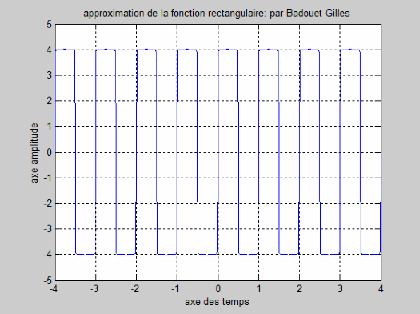
1.1 Addition progressive de plusieurs harmoniques de la
série de Fourier à l'aide d'un code MATLAB jusqu'à
obtention de la ou d'une fonction qui se rapproche de la fonction
rectangulaire.
Formule généralisée de la fonction
rectangulaire :
n
Rect. (t) =? dk . (Cos (k.w.t) + sin (k.w.t)) =
4/Ð.Vmax.(sin(w.t) +
K=1
1/3.sin (3w.t) +...+ 1/ (2k+1).Sin ((2k+1)
w.t)
code MATLAB:
clear all;
close all;
t=5:0.01:10 vmax=100;
f=1 ;
w=2*p*fi;
Rect = 0;
for k=0:900
Rect= Rect+ ((4/pi)*vmax)*(1/
(2*k+1))*sin
((2*k+1)*w*t);
end
pPlot (t, Rect,'m')
On obtient le graphe ci-dessous:
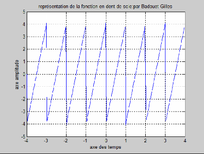
1.2 Représentation graphique de la série
de Fourier d'une fonction en dent
de scie
Expression de la fonction en dent de scie :
d(t) = (12 2 ð) Vmax . (sin(wt) + 1/2.sin(2wt) +
(1,3) sin (3wt) + ...
+ (1ik) sin (kwt) ) ; k n
Le code MATLAB :
clear all; close all; vmax=20; f=1;
w=2*pi*f;
t=-1.5:0.01:7;
D (t) =0;
for k=1:800
D (t) = D (t) + (12/pi)*vmax*(sin (k*w*t)/k);
end
plot (t, D (t),'r');
Graphe:
TP2: Analyse des systèmes linéaires au
spectre des fréquences
(représentation de BODE et de nYQYUIST
d'une fonction de
transfert)
Soit la fonction de transfert suivante: H(s) = z(s) / n(s) =
(s2-2s+3) / (s3+3s2+1) En langage MATLAB son
écriture sera : H(s) = z(s) / n(S) = (s. A2-2*s+3)/ (s.
A3+3*s. A2+1)
2.1 Code du vecteur z sous forme z = Ia3 a2 a1 a0] et
également celui de n
|
z= 10
|
1
|
-2
|
3];
|
|
n= 11
|
3
|
0
|
1];
|
2.2 Verifier que le code : Printsys (z, n) affiche la
fonction de transfert H sur l'ecran
Code :
|
z= [0
|
1
|
12
|
3];
|
|
n= [1
|
3
|
0
|
1];
|
printsys (z, n)
Le resultat est le suivant:
num/den = (SA2 - 2 s + 3)/(SA3 + 3 sA2 + 1)
2.3 Calcul du gain statique H (0)
Code :
|
z=[0
|
1
|
12
|
3];
|
|
n=[1
|
3
|
0
|
1];
|
dcgain (z, n) solution:
ans =
3
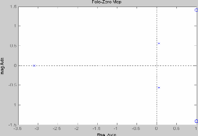
2.4 Représentation graphique des pôles et
des zéros de H :
Code :
|
z= 10
|
1
|
-2
|
3];
|
|
n= (1
|
3
|
0
|
1];
|
pzmap (z, n)
Graphe :
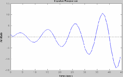
2.5 Representation graphic:ue de la reponse
impulsionnelle
Code :
|
z=10
|
1
|
-2
|
3];
|
|
n=11
|
3
|
0
|
1];
|
Impulse(z,n)
Graphe :
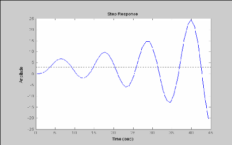
Representation graphic:ue de la reponse a la fonction
de
Heaviside du systeme
code :
|
z= [0
|
1
|
-2
|
3];
|
|
n= [1
|
3
|
0
|
1];
|
Step (z. n)
Graphe :
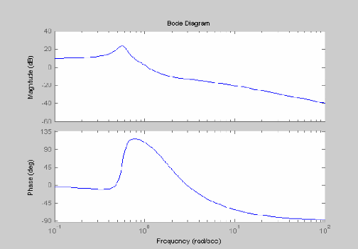
2.7 Representation graphic:ue du diagramme de
Bode code:
|
z= [0
|
1
|
-2
|
3];
|
|
n= [1
|
3
|
0
|
1];
|
bode (z, n)
graphe:
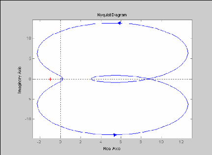
eoresentation qraohique de la courbe d'espace de
nyquist
code:
|
z= [0
|
1
|
-2
|
3];
|
|
n= [1
|
3
|
0
|
1];
|
nyquist (z, n) graphe:
II PARTIE: Travail Pratique N2
EXERCICE
n=[5 1];
impulse=[1,zeros(1,5)];pulsetrain=[1,zeros(1,n)];
pulsetrain=[1,zeros(1,5)];
pulsetrain=[pulsetrain pulsetrain pulsetrain pulsetrain
pulsetrain]; step=[ones(1,50)]; phi=pi/20;
imagexp=[exp(j*(0:49)*phi)];
subplot(2,2,1);stem(impulse);
subplot(2,2,2);stem(pulsetrain);
subplot(2,2,3);stem(step);
subplot(2,2,4);stem(real(imagexp)); hold on;
stem(imag(imagexp));
a) Expliquer la fonction de chaque Commande :
impulse=[1,zeros(1,5)];
Stimule la réponse impulsionnelle d'un système de
t=1 à t=5
Résultat : impulse =
1 0 0 0 0 0
pulsetrain=[1,zeros(1,n)];
Permet d'obtenir une impulsion. La dite impulsion est
constitué d'un pic de tension (1) et d'un repos de n unités de
temps. nous avons pris dans ce cas n=5.
Résultat :
pulsetrain =
1 0 0 0 0 0
pulsetrain=[pulsetrain pulsetrain pulsetrain pulsetrain
pulsetrain]; Permet d'obtenir une série de 5 impulsions.
Résultat :
pulsetrain =
Columns 1 through 10
|
1 0 0 0 0 0
|
1
|
0
|
0
|
0
|
|
Columns 11 through 20
0 0 1 0 0 0
|
0
|
0
|
1
|
0
|
Columns 21 through 30
0 0 0 0 1 0 0 0 0 0
step=[ones(1,50)];
Stimule la réponse d'un système LTI de t=1 à
t=50 Résultat :
step =
Columns 1 through 10
|
1 1 1 1 1 1
|
1
|
1
|
1
|
1
|
|
Columns 11 through 20
1 1 1 1 1 1
|
1
|
1
|
1
|
1
|
|
Columns 21 through 30
1 1 1 1 1 1
|
1
|
1
|
1
|
1
|
|
Columns 31 through 40
1 1 1 1 1 1
|
1
|
1
|
1
|
1
|
|
Columns 41 through 50
1 1 1 1 1 1
|
1
|
1
|
1
|
1
|
imagexp=[exp(j*(0:49)*phi)];
Renvoie le module la fonction exp(j*k*phi) quelque soit k
appartenant à [0 ; 49] avec phi = ð/20.
Résultat :
imagexp =
Columns 1 through 3
1.0000 0.9877 + 0.1564i 0.9511 + 0.3090i
Columns 4 through 6
0.8910 + 0.4540i 0.8090 + 0.5878i 0.7071 + 0.7071i
Columns 7 through 9
|
0.5878 + 0.8090i 0.4540
|
+ 0.8910i
|
0.3090
|
+ 0.9511i
|
|
Columns 10 through 12
|
|
|
|
|
0.1564 + 0.9877i 0.0000
|
+ 1.0000i
|
-0.1564
|
+ 0.9877i
|
|
Columns 13 through 15
|
|
|
|
|
-0.3090 + 0.9511i -0.4540
|
+ 0.8910i
|
-0.5878
|
+ 0.8090i
|
|
Columns 16 through 18
|
|
|
|
|
-0.7071 + 0.7071i -0.8090
|
+ 0.5878i
|
-0.8910
|
+ 0.4540i
|
|
Columns 19 through 21
|
|
|
|
|
-0.9511 + 0.3090i -0.9877
|
+ 0.1564i
|
-1.0000
|
+ 0.0000i
|
|
Columns 22 through 24
|
|
|
|
|
-0.9877 - 0.1564i -0.9511
|
- 0.3090i
|
-0.8910
|
- 0.4540i
|
|
Columns 25 through 27
|
|
|
|
|
-0.8090 - 0.5878i -0.7071
|
- 0.7071i -0.5878
|
- 0.8090i
|
|
Columns 28 through 30
|
|
|
|
|
-0.4540 - 0.8910i -0.3090
|
- 0.9511i
|
-0.1564
|
- 0.9877i
|
|
Columns 31 through 33
|
|
|
|
|
-0.0000 - 1.0000i 0.1564
|
- 0.9877i
|
0.3090
|
- 0.9511i
|
|
Columns 34 through 36
|
|
|
|
|
0.4540 - 0.8910i 0.5878
|
- 0.8090i
|
0.7071
|
- 0.7071i
|
|
Columns 37 through 39
|
|
|
|
|
0.8090 - 0.5878i 0.8910
|
- 0.4540i
|
0.9511
|
- 0.3090i
|
|
Columns 40 through 42
|
|
|
|
|
0.9877 - 0.1564i 1.0000
|
- 0.0000i
|
0.9877
|
+ 0.1564i
|
Columns 43 through 45
Résultat :
0.9511 + 0.3090i 0.8910
|
+ 0.4540i
|
0.8090
|
+ 0.5878i
|
|
Columns 46 through 48
|
|
|
|
|
0.7071 + 0.7071i 0.5878
|
+ 0.8090i
|
0.4540
|
+ 0.8910i
|
|
Columns 49 through 50
|
|
|
|
|
0.3090 + 0.9511i 0.1564
|
+ 0.9877i
|
|
|
H = SUBPLOT(m,n,p)
Permet de représenter des graphiques dans une matrice m
sur n, et représente la figure courante à la P ième
position.
:
>> m=5; >> n=8; >> p=2; >> H = subplot
(m,n,p)
Résultat :

subplot (2 ,2 ,1) ; stem(impulse) ;
Affiche les séquences de données de Y comme des
segments partant de l'axe des abscisses et terminés par des cercles pour
des valeurs de données. Si Y est un tableau, alors chaque colonne est
représentée par une série séparée

subplot (2 ,2 ,2) ; stem(pulsetrain) ;
subplot (2 ,2 ,3) ; stem(step) ;
subplot (2 ,2 ,4) ; stem(real (imagexp)); hold on; stem
(imag(imagexp));
b) Afficher les quatre séquences
numériques


10 20 30


1 0.8 0.6 0.4 0.2
0
1 0.8 0.6 0.4 0.2
0
2 4 6
|
1 0.8 0.6
|
|
|
|
|
|
1
0.5
0
-0.5
-1
|
|
|
|
|
|
|
|
|
|
0.4
0.2
0
|
|
|
|
|
|
|
|
|
0 20 40 60
0 20 40 60
- 18 -
III Partie Travail Pratique N3 : Conversion
de modèles
Conversion d'un model état à un model de
la fonction de transfert
Code :
sys_tf=tf(1.5, [1 9 30.6])
ésultat:
Transfer function: 1.5
s^2 + 9 s + 30.6
conversion en modele zpk
code
sys_zpk=zpk([0, -2], [4, 3.6], 9)
ésultat:
Zero/pole/gain: 9 s (s+2)
(s-4) (s-3.6)
Affichage des paramètres
Code:
a=3; b=7; c=1; d=11;
sys=ss(a,b,c,d)
Résultat:
a =
x1
x1 3
b=
u1
x1 7
c =
x1
y1 1
d=
u1
y1 11
Continuous-time model.
- 20 -
Simulation d'un modèle d'espace
Considérons le système LTI ci-dessous :
UL UR


i1
UC
U1
i2
i3
U2
1) X(I,U) ; dX /dt = AX + B A et B étant des matrices.
2) Y= CX+D C et D étant des matrices.
Donnons des valeurs à nos matrices.
Etude
Apres étude de ce système on obtient l'expression
suivante
En posant X= (i1 ;u2)
. dX= (R/L 1/L ; 1/C 0) * X + (-1/L ; 0) U1.
Par correspondance avec l'expression .dX= Ax +BU1
On obtient et les matrices suivantes A= (R/L 1/L ; 1/C 0)
B= (-1/L ; 0)
Par ailleurs, U2=U2 donc,
U2= (0 ; 1) (i1 ; U2)
Par correspondance avec l'expression
U2= CX + D On Obtient C= (0 ; 1)
D= (0)
Choisissons R=5 ohms L= 10H
C=50mF
Donc
A= (0.5 0.1 ; 20 0)
B= (-0.1 ; 0) C= (0 ; 1)
D= (0)
Simuler un modèle d'espace de mon choix
Soit les matrices a, b, c et d
Code:
a=[-.8 2 ;-2 -.8];
b=[1 .2;.9 1];
c=[1 0];
d=[.2 1];
subplot(2,2,1); pzmap(a,b,c,d)
subplot(2,2,2); impulse(a,b,c,d)
subplot(2,2,3); step(a,b,c,d)
subplot(2,2,4); initial(a,b,c,d)
ésultat:


IV Partie Travail Pratique N4: Fonction d'erreur de
Gauss
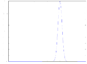
Code:
e=8;
t=[-10:0.01:10];
g=(exp(-t.^2/ sqrt(e*pi))/sqrt(e*pi);
plot(t,g,'r'); xlabel('temps t');
ylabel('g');
gtext('la fonction erreur de Gauss');
ésultat :
e=8;
t=[-30:0.01:30];
u=10;
f=(exp(-(t-u).^2/sqrt(e*pi))/sqrt(e*pi)); z=plot(t,f,'b')
xlabel('temps t');
ylabel('g');
Chemin inverse de l'obtention de la function de
gauss
A = [f]
fid = fopen('fich.m','r+') : ouverture du fichier en mode
lecture/écriture
count = fwrite(fid,f) : écriture dans le fichier des
valeurs de la fonction f
fclose(fid) : fermeture du fichier
save gausserror : sauvegarde du fichier contenant le code sous
Matlab
load gausserror : chargement en mémoire de ce fichier
gausserror : validation et exécution
Réponse : z =
152.0133
A =
Columns 1 through 5
|
0.0000 0.0000 0.0000
|
0.0000
|
0.0000
|
|
Columns 6 through 10
|
|
|
|
0.0000 0.0000 0.0000
|
0.0000
|
0.0000
|
|
Columns 11 through 15
|
|
|
|
0.0000 0.0000 0.0000
|
0.0000
|
0.0000
|
|
Columns 16 through 20
|
|
|
|
0.0000 0.0000 0.0000
|
0.0000
|
0.0000
|
|
Columns 21 through 25
|
|
|
|
0.0000 0.0000 0.0000
|
0.0000
|
0.0000
|
Columns 26 through 30
|
0.0000 0.0000 0.0000
|
0.0000
|
- 25 -
0.0000
|
|
Columns 31 through 35
|
|
|
|
0.0000 0.0000 0.0000
|
0.0000
|
0.0000
|
|
Columns 36 through 40
|
|
|
|
0.0000 0.0000 0.0000
|
0.0000
|
0.0000
|
|
Columns 41 through 45
|
|
|
|
0.0000 0.0000 0.0000
|
0.0000
|
0.0000
|
|
Columns 46 through 50
|
|
|
|
0.0000 0.0000 0.0000
|
0.0000
|
0.0000
|
|
Columns 51 through 55
|
|
|
|
0.0000 0.0000 0.0000
|
0.0000
|
0.0000
|
|
Columns 56 through 60
|
|
|
|
0.0000 0.0000 0.0000
|
0.0000
|
0.0000
|
|
Columns 61 through 65
|
|
|
|
0.0000 0.0000 0.0000
|
0.0000
|
0.0000
|
|
Columns 66 through 70
|
|
|
|
0.0000 0.0000 0.0000
|
0.0000
|
0.0000
|
|
Columns 71 through 75
|
|
|
|
0.0000 0.0000 0.0000
|
0.0000
|
0.0000
|
|
Columns 76 through 80
|
|
|
|
0.0000 0.0000 0.0000
|
0.0000
|
0.0000
|
|
Columns 81 through 85
|
|
|
|
0.0000 0.0000 0.0000
|
0.0000
|
0.0000
|
Columns 86 through 90
|
0.0000 0.0000 0.0000
|
0.0000
|
- 26 -
0.0000
|
|
Columns 91 through 95
|
|
|
|
0.0000 0.0000 0.0000
|
0.0000
|
0.0000
|
|
Columns 96 through 100
|
|
|
|
0.0000 0.0000 0.0000
|
0.0000
|
0.0000
|
|
Columns 101 through 105
|
|
|
|
0.0000 0.0000 0.0000
|
0.0000
|
0.0000
|
|
Columns 106 through 110
|
|
|
|
0.0000 0.0000 0.0000
|
0.0000
|
0.0000
|
|
Columns 111 through 115
|
|
|
|
0.0000 0.0000 0.0000
|
0.0000
|
0.0000
|
|
Columns 116 through 120
|
|
|
|
0.0000 0.0000 0.0000
|
0.0000
|
0.0000
|
|
Columns 121 through 125
|
|
|
|
0.0000 0.0000 0.0000
|
0.0000
|
0.0000
|
|
Columns 126 through 130
|
|
|
|
0.0000 0.0000 0.0000
|
0.0000
|
0.0000
|
|
Columns 131 through 135
|
|
|
|
0.0000 0.0000 0.0000
|
0.0000
|
0.0000
|
|
Columns 136 through 140
|
|
|
|
0.0000 0.0000 0.0000
|
0.0000
|
0.0000
|
|
Columns 141 through 145
|
|
|
|
0.0000 0.0000 0.0000
|
0.0000
|
0.0000
|
|
Columns 146 through 150
|
|
- 27 -
|
|
0.0000 0.0000 0.0000
|
0.0000
|
0.0000
|
|
Columns 151 through 155
|
|
|
|
0.0000 0.0000 0.0000
|
0.0000
|
0.0000
|
|
Columns 156 through 160
|
|
|
|
0.0000 0.0000 0.0000
|
0.0000
|
0.0000
|
|
Columns 161 through 165
|
|
|
|
0.0000 0.0000 0.0000
|
0.0000
|
0.0000
|
|
Columns 166 through 170
|
|
|
|
0.0000 0.0000 0.0000
|
0.0000
|
0.0000
|
|
Columns 171 through 175
|
|
|
|
0.0000 0.0000 0.0000
|
0.0000
|
0.0000
|
|
Columns 176 through 180
|
|
|
|
0.0000 0.0000 0.0000
|
0.0000
|
0.0000
|
|
Columns 181 through 185
|
|
|
|
0.0000 0.0000 0.0000
|
0.0000
|
0.0000
|
|
Columns 186 through 190
|
|
|
|
0.0000 0.0000 0.0000
|
0.0000
|
0.0000
|
|
Columns 191 through 195
|
|
|
|
0.0000 0.0000 0.0000
|
0.0000
|
0.0000
|
|
Columns 196 through 200
|
|
|
|
0.0000 0.0000 0.0000
|
0.0000
|
0.0000
|
|
Columns 201 through 205
|
|
|
|
0.0000 0.0000 0.0000
|
0.0000
|
0.0000
|
|
Columns 206 through 210
|
|
- 28 -
|
|
0.0000 0.0000 0.0000
|
0.0000
|
0.0000
|
|
Columns 211 through 215
|
|
|
|
0.0000 0.0000 0.0000
|
0.0000
|
0.0000
|
|
Columns 216 through 220
|
|
|
|
0.0000 0.0000 0.0000
|
0.0001
|
0.0001
|
|
Columns 221 through 225
|
|
|
|
0.0002 0.0002 0.0004
|
0.0006
|
0.0009
|
|
Columns 226 through 230
|
|
|
|
0.0014 0.0020 0.0029
|
0.0042
|
0.0059
|
|
Columns 231 through 235
|
|
|
|
0.0082 0.0112 0.0150
|
0.0199
|
0.0259
|
|
Columns 236 through 240
|
|
|
|
0.0331 0.0418 0.0518
|
0.0632
|
0.0760
|
|
Columns 241 through 245
|
|
|
|
0.0898 0.1045 0.1197
|
0.1349
|
0.1497
|
|
Columns 246 through 250
|
|
|
|
0.1634 0.1756 0.1856
|
0.1932
|
0.1979
|
|
Columns 251 through 255
|
|
|
|
0.1995 0.1979 0.1932
|
0.1856
|
0.1756
|
|
Columns 256 through 260
|
|
|
|
0.1634 0.1497 0.1349
|
0.1197
|
0.1045
|
Columns 261 through 265
|
0.0898 0.0760 0.0632
|
0.0518
|
- 29 -
0.0418
|
|
Columns 266 through 270
|
|
|
|
0.0331 0.0259 0.0199
|
0.0150
|
0.0112
|
|
Columns 271 through 275
|
|
|
|
0.0082 0.0059 0.0042
|
0.0029
|
0.0020
|
|
Columns 276 through 280
|
|
|
|
0.0014 0.0009 0.0006
|
0.0004
|
0.0002
|
|
Columns 281 through 285
|
|
|
|
0.0002 0.0001 0.0001
|
0.0000
|
0.0000
|
|
Columns 286 through 290
|
|
|
|
0.0000 0.0000 0.0000
|
0.0000
|
0.0000
|
|
Columns 291 through 295
|
|
|
|
0.0000 0.0000 0.0000
|
0.0000
|
0.0000
|
|
Columns 296 through 300
|
|
|
|
0.0000 0.0000 0.0000
|
0.0000
|
0.0000
|
|
Columns 301 through 305
|
|
|
|
0.0000 0.0000 0.0000
|
0.0000
|
0.0000
|
|
Columns 306 through 310
|
|
|
|
0.0000 0.0000 0.0000
|
0.0000
|
0.0000
|
|
Columns 311 through 315
|
|
|
|
0.0000 0.0000 0.0000
|
0.0000
|
0.0000
|
|
Columns 316 through 320
|
|
|
|
0.0000 0.0000 0.0000
|
0.0000
|
0.0000
|
Columns 321 through 325
|
0.0000 0.0000 0.0000
|
0.0000
|
- 30 -
0.0000
|
|
Columns 326 through 330
|
|
|
|
0.0000 0.0000 0.0000
|
0.0000
|
0.0000
|
|
Columns 331 through 335
|
|
|
|
0.0000 0.0000 0.0000
|
0.0000
|
0.0000
|
|
Columns 336 through 340
|
|
|
|
0.0000 0.0000 0.0000
|
0.0000
|
0.0000
|
|
Columns 341 through 345
|
|
|
|
0.0000 0.0000 0.0000
|
0.0000
|
0.0000
|
|
Columns 346 through 350
|
|
|
|
0.0000 0.0000 0.0000
|
0.0000
|
0.0000
|
|
Columns 351 through 355
|
|
|
|
0.0000 0.0000 0.0000
|
0.0000
|
0.0000
|
|
Columns 356 through 360
|
|
|
|
0.0000 0.0000 0.0000
|
0.0000
|
0.0000
|
|
Columns 361 through 365
|
|
|
|
0.0000 0.0000 0.0000
|
0.0000
|
0.0000
|
|
Columns 366 through 370
|
|
|
|
0.0000 0.0000 0.0000
|
0.0000
|
0.0000
|
|
Columns 371 through 375
|
|
|
|
0.0000 0.0000 0.0000
|
0.0000
|
0.0000
|
|
Columns 376 through 380
|
|
|
|
0.0000 0.0000 0.0000
|
0.0000
|
0.0000
|
|
Columns 381 through 385
|
|
- 31 -
|
|
0.0000 0.0000 0.0000
|
0.0000
|
0.0000
|
|
Columns 386 through 390
|
|
|
|
0.0000 0.0000 0.0000
|
0.0000
|
0.0000
|
|
Columns 391 through 395
|
|
|
|
0.0000 0.0000 0.0000
|
0.0000
|
0.0000
|
|
Columns 396 through 400
|
|
|
|
0.0000 0.0000 0.0000
|
0.0000
|
0.0000
|
Column 401
0.0000
fid =
+1
-30 -20 -10 0 10 20 30
g
0.18
0.16
0.14
0.12
0.08
0.06
0.04
0.02
0.2
0.1
0
temps t


