Comparison of process mining techniques application to flexible and unstructured processes

Introduction

of different mining algorithms implementation. We shows that it is possible to get much more information's by applying some analysis techniques on the mining results. Another very important kind of plug-ins which provide to ProM the ability to convert one model into another model is also presented.

In the third chapter analyze and compare process mining algorithms against a known ground truth, using the ProM framework. The analysis concerns three mining algorithms, namely: the Alpha algorithm, Heuristic algorithm and Genetic algorithm, according to the metrics presented in the chapter 1.

Finally, in the chapter 4 we present our approach to traces clustering with some experimentation results. Then, we conclude this thesis by a short conclusion and some perspectives.

4

Chapter1

Business Process and Process Mining

1.1 Introduction

In this chapter we introduce the main aspects of Business Process (BP) and Process Mining (PM) field. We present these two inherently related field following three main sections. The first section (Section 1.2) is devoted to the basic notions of Business Process. Indeed, we begin this section by giving some definitions, the BP life cycle then some BP modeling languages. In the second section (Section 1.3) we present an overview of the Process Mining filed. Indeed, in this part we present different related aspects to the Process Mining like: Event Logs, Log filtering and Process Mining Perspectives. After that, we expose some notions related to the Control-Flow Discovery algorithms. In the third section, we describe some evaluation approaches of business processes (Section 1.4). We expose in this section different evaluation metrics.

1.2 Business Processes

The term "business process" is often used to refer to different concepts such as : abstract process, executable process or collaborative process [54]. A business process is a choreography of activities including an interaction between participants in the form of exchange of information. Participants can be:

· Applications / Services Information System,

· Human actors,

· Other business processes.

5

Business Process and Process Mining

1.2.1 Definitions

Different definitions were given to the business process in the literature. In [13], the authors consider that a business process is :

A collection of activities that takes one or more kinds of input and creates an output that is of value to the customer. A business process has a goal and is affected by events occurring in the external world or in other processes.

A more formal definition were given by [1],

A business process P is defined as a set of activities V_p = {V1, V2, ...V_n}, a directed graph G_p = (V_p, E_p), an output function op:Vp -? N^k and V(u, v) E E_p a boolean function fu,v= Nk -? 0, 1.

In this case, the process is constructed in the following way: for every completed activity u, the value _op(u) is calculated and then, for every other activity v, if fu,v(op(u)) is "true", v can be executed.

A business process can be internal to a company or involves business partners. This is called collaborative process. A collaborative process is a business process involving partner companies. A collaborative process involving n partners is composed of two parts: an interface and n implementations. The interface defines the visible part of the process, this represent the contract between the partners: definition of the business exchanged documents, sequencing of activities, roles and responsibilities of each partner. The specific implementation of each partner is abstract because of this interface. Implementations (one for each partner) define internal behavior of each partner to achieve the process and respect the constraints defined in the public interface.

In a company a business process includes several basic aspects that can be modeled and processed independently (Figure 1.1). According to the authors in [19], these aspects can be grouped in the following items :

· Organizational Aspect: It describes the organizational structure of the company (departments, services, etc..) that is invoked for the achievement of business processes through the concepts of role, roles group, actor (or agent ), team, etc.

· Informational Aspect: It describes the information (data, documents, etc..) that are manipulated by the user (or actor) of business process to execute an activity or process.

· Behavioral Aspect: It corresponds to the modeling of the dynamics of business processes, ie, the way that the activities are chronologically performed and the triggering conditions.

6

Business Process and Process Mining

· Operational Aspect: It describes all the activities involved in a business process.

· Functional Aspect: It describes the objective of the business process.

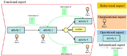
Figure 1.1: Different aspects of a business process [54]

1.2.2 Business Process Management

The efforts to help organizations, in many areas of business, to manage their process changes have given rise to a new kind of systems, called 'Business Process Management' (BPM) systems [1]. They have been widely used and are the best methodology so far. The increasing use of such systems in companies expresses their undeniable importance as a tool for automation of their process. Business Process Management Systems are among the most elaborate systems to define and execute processes. They allow, in particular, to explicitly describe the methods of carrying out a work process, to experiment, to measure their quality and to optimize them in order to ensure the improvement and the reuse of processes [54].

1.2.3 BPM life cycle

The BPM process goes through different phases. The figure (1.2), illustrate the classical BPM life cycle. The first phase in this life cycle is the process design phase which is followed by the process configuration phase, in which, the design is used to configure some process-aware information system in the configuration phase. After the process has been running for a while in the enactment phase (process enactment) and event logs have

7

Business Process and Process Mining

been collected, diagnostics can be used to develop another (and preferably better) design (process diagnosis).

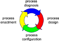
Figure 1.2: BPM life cycle [15].

Adopting this approach is assuming that large information systems are expected to evolve over time into larger and better systems. In practice, processes are often implicit (i.e. they are not designed as such, but emerged from daily practice) or not enforced by any system. However, when these processes are analyzed, they can be captured by one or different process models of some sort. Obviously, when capturing and making a process model, mistakes should be avoided. For that, it is very important to adopt a clear and reliable business model. This will ensure some important benefits like:

· The possibility to increase the visibility of the activities, that allows the identification of problems (e.g. bottlenecks) and areas of potential optimization and improvement;

· The ability to group the activities in "department" and persons in "roles", in order to better define duties, auditing and assessment activities.

So, following the previous listed benefits, a process model should be built around some basic characteristics. The most important one is that a model should be unambiguous in the sense that the process is precisely described without leaving uncertainties to the potential reader.

1.2.4 Business processes modeling languages

It exist many languages for business processes modeling. The most used languages for the specification of business processes are those with a graph-based representations formalisms. The nodes represent the process's tasks (or, in some notations, also the states

8

Business Process and Process Mining

and the possible events of the process), and arcs represent ordering relations between tasks (for example, an arc from node n1 to n2 represents a dependency in the execution so that n2 is executed only after n1 ). The most used and adopted graph based languages are: Petri nets [17, 55] and BPMN [33].

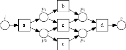
1.2.4.1 Petri Nets

Petri Nets are a formal language that can be used to specify processes. Since the language has a formal and executable semantics, processes modeled in terms of a Petri Net can be executed by an information system.

Definition (Petri Net). The authors in [41] have defined Petri Net as follow:

A Petri Net is a tuple (P, T, F). where: P is a finite set of places; T is a finite set of transitions, such that P n T = n and F c (P x T) U (T x P) is a set of directed arcs, called flow relation.

A Petri Net is a directed graph composed of two types of nodes: places and transitions. Usually, places are represented as circles and transitions are represented as rectangles. Petri Nets are bipartite graphs, meaning that an arc in the net may connect a place to a transition or vice-versa, but no arc may connect a place to another place or a transition to another transition. A transition has a number of immediately preceding places (called its input places) and a number of immediately succeeding places (called its output places) [24]. The network structure is static, but, governed by the firing rule, tokens can flow through the network. The state of a Petri Net is determined by the distribution of tokens over places and is referred to as its marking. In the initial marking shown in (Figure 1.3), there is only one token, start is the only marked place. Petri Nets are particularly suited for the systems behavior modeling in terms of "flow" (the flow of control or flow of objects or information) and offer an intuitive visualization of the process model. They have been studied from a theoretical point of view for several decades, which had led to a number of tools that enable their automated analysis.

9

Business Process and Process Mining

Figure 1.3: A marked Petri net.

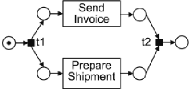
Places are containers for tokens and tokens represent the thing(s) that flow through the system. During the execution of a Petri Net and at a given point, each place may hold zero, one or multiple tokens. Functions are used to represent Petri Net states by assigning a number of tokens to each place in the net. Such functions are called a marking. For example, (Figure 1.4 (i)) depicts a marking of a Petri Net where there is one token in the leftmost place and no token in any other place. The state of a Petri Net changes when one of its transitions fires. A transition may only fire if there is at least one token in each of its input places. In this case, we say that the transition is enabled.

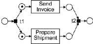
For instance, in (Figure 1.4(a)), the transition labeled t1 is enabled since this transition has only one input place and this input place has one token. When a transition fires, it removes one token from each of its input places and it adds one token to each of its output places. For example, (Figure 1.4 (b)) depicts the state obtained when transition t1 fires starting from the marking in (Figure 1.4 (a)). The token in the leftmost place has been removed, and a token has been added to each of the output places of transition t1. In a given marking, there may be multiple enabled transitions simultaneously.

In this situation, any of these enabled transitions may fire at any time. For example, in (1.4 (b)) there are two transitions enabled: "Send Invoice" and "Prepare Shipment". Any of these transitions may fire in the next execution step. Note that when the label attached to a transition is long (e.g. "Send Invoice") we place the label inside the rectangle representing this transition. Also, we will sometimes omit the label of a transition altogether. Transitions without labels correspond to "silent steps" which have no effect on the outside world, as opposed to a transition such as "Send Invoice".

Business Process and Process Mining

(a) Petri nets in an initial marking

(b) Petri nets after transition t1 fires

Figure 1.4: Petri Nets in two different states.

An important subclass of Petri Nets is the Workflow Nets (WF-Net), whose most important characteristic is to have a dedicated "start" and "end".

1.2.4.2 Workflow Nets

Workflow Nets, or WF-Nets, are a subclass of Petri nets, tailored towards workflow modeling and analysis. For example in [49], several analysis techniques are presented towards soundness verification of WF-nets.

Basically, WF-nets correspond to P/T-nets with some structural properties. These structural properties aims at clearly seeing the initial and final state for each executed case. Furthermore, they ensure that there are no unreachable parts of the model, i.e.:

· The initial marking marks exactly one place (the initial place or source place), and this place is the only place without incoming arcs,

· There is exactly one final place or sink place, i.e. a place without outgoing arcs,

· Each place or transition is on a path that starts in the initial place and ends in the final place.

10

Formally, WF-Nets are defined as follows:

Business Process and Process Mining

Definition 1.2.1. (Workflow Net)

A P/T-net g = (P, T, F) is a workflow Net (or WF-Net) if and only if:

There exists exactly one pj E P, such that
·pj = 0, i.e. the source place, There exists exactly one pf E P, such that pf
· = 0, i.e. the sink place, Each place and transition is on a path from pj to pf .

11

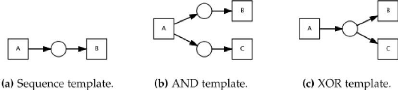
Figure 1.5: Some basic workflow templates that can be modeled using Petri Net notation.

In the literature, there have been proposed various correctness criteria for Workflow Nets [26]. One of the most used criterion is soundness, which is defined as follows:

Definition 1.2.2. (Classical Soundness) Let N= (P, T, F, A, l) be a Workflow Net with input place j and output place o. N is sound if and only if:

· Safeness: (N, [j]) is safe, i.e., places cannot hold multiple tokens at the same time.

· Proper completion: for any marking M E [N, [j]], o E M implies M = [o].

· Option to complete: for any marking M E [N, [j]] , [o] E [N, M].

· Absence of dead parts: (N, [j]) contains no dead transitions (i.e., for any t E T ,there is a firing sequence enabling t).

1.2.4.3 Causal Nets (C-Nets)

To represent activities, process modeling languages have typical elements, but often they also have extra elements to specify the relation between activities (semantics). For instance, to represent states of the process and to model the control-flow, Petri Net requires

12

Business Process and Process Mining

places. BPMN has gateways and events. All of these extra elements do not leave a trace in event logs, i.e., no events are generated by occurrence of elements other than the ones representing activities. Thus, given an event log, process discovery techniques must also "guess" the existence of such elements in order to describe the observed behavior in the log correctly. This causes several problems as the discovered process model is often unable to represent the underlying process well, e.g., the model is overly complex because all kinds of model elements need to be introduced without a direct relation to the event log (e.g., places, gateways, and events) [44]. Furthermore, generic process modeling languages often allow for undesired behavior such as deadlocks and live-locks.

Figure 1.6: A causal net example.

Causal nets are a process model representation tailored towards process mining [44]. In causal net, activities are represented by nodes and the dependencies between them are represented by arcs. Each causal net is characterized by a start and end activity. The activities semantics' are shown by their input and output bindings.

1.2.4.4 BPMN

Multiple tool vendors have been in need for a unique standardization of a single notation to Business Process Modeling. They have made an agreement among them and they have proposed the Business Process Modeling and Notation) [33]. As a benefit of BPMN, it is used in many real cases and many tools adopt it daily. BPMN provides a graphical notation to describe business processes, which is both intuitive and powerful (it is able to represent complex process structure). It is possible to map a BPMN diagram to an execution language, BPEL (Business Process Execution Language)¹.

'Business Process Execution Language (BPEL), short for Web Services Business Process Execution Language (WS-BPEL) is an OASIS standard executable language for specifying actions within business

processes with web services. Processes in BPEL export and import information by using web service interfaces exclusively

Business Process and Process Mining

13

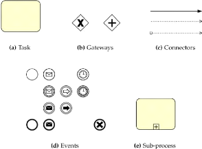
Figure 1.7: Example of some basic components, used to model a business process using BPMN notation.

The main components of a BPMN diagram (Figure 1.7) are as follow:

Events: an event is defined as something that "happens" during the course of a process; typically an event has a cause (trigger) and an impact (result). Each event is represented with a circle (containing an icon, to specify some details), as in Figure (1.7 (d)). It exist three types of events: start (single narrow border), intermediate (single thick border) and end (double narrow border).

Activities: The work done by a company is identified by a generic term which is Activity. In the graphical representation, rounded rectangles are used to identify activities. There are few types of activity like tasks (a single unit of work, (Figure 1.7 (a))) and subprocesses (used to hide different levels of abstraction of the work, (Figure 1.7 (e))).

Gateway: A Gateway is used as a structure to control the divergences and convergences of the flow of the process (fork, merge and join). Internal markers like (exclusive, event based, inclusive, complex and parallel) are used to identify the type of gateway, like "exclusive" (Figure 1.7 (b)).

Sequence and message flows and associations : They are used as connectors between components of the graph. The order of the activities is indicated by a sequence flow (Figure 1.7 (c),top). The flow of the messages (as they are prepared,

14

Business Process and Process Mining

sent and received) between participants is shown by a Message Flow (Figure 1.7 (c),bottom). Associations (Figure 1.7 (c), middle) are used to connect artifacts with other elements of the graph.

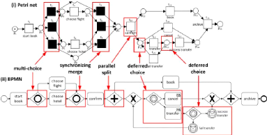
Figure 1.8: A Petri Net and a BPMN model that exhibit similar set of traces, annotated with some control-flow patterns that exist in both models.

Unlike Petri Nets, BPMN provides abundance of notations to represent complex patterns. For example in Figure (1.8), both multi-choice and synchronizing merge patterns are each represented by a dedicated gateway. There are many ways to express the same behavior in BPMN. As illustrated in Figure (1.8) it is possible to represent the same deferred choice pattern by two different alternatives: using tasks with type "receive", or using events. Despite of its popular use, BPMN also has some drawbacks, for instance, the states are not explicitly defined.

1.3 Process Mining

Process mining is the art of extracting non-trivial and useful information about processes from event logs. As illustrated in Figure (1.9), process mining closes the process modeling loop by allowing the discovery, analysis and extension of (process) models from event logs. One aspect of process mining is control-flow discovery, i.e., automatically constructing a process model which describes the causal dependencies between activities [45]. The basic idea of control-flow discovery is very simple: it consist on automatically construct a suitable process model "describing the behavior" from a given event log containing a set of traces. The second aspect is the organizational aspect, which focuses on who performed

15

Business Process and Process Mining

which actions [47]. This can give insights in the roles and organizational units or in the relations between individual performers (i.e. a social network).

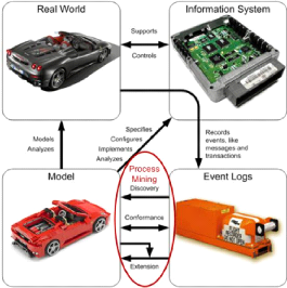
Figure 1.9: From event logs to models via process mining

1.3.1 Event logs

An event log consists of events that pertain to process instances. A process instance is defined as a logical grouping of activities whose state changes are recorded as events. An Event logs shows occurrences of events at specific moments in time, where each event refers to a specific process and an instance thereof, i.e. a case. An Event log could show the events that occur in a specific machine that produces computer chips, or it could show the different departments visited by a patient in a hospital. Event logs, serves as a basis for process analysis. It assumes that it is possible to record events such that:

1. Each event refers to an activity (i.e., a well-defined step in the process);

2. Each event refers to a case (i.e., a process instance);

3. Each event can have a performer also referred to as originator (the actor executing or initiating the activity);

4. Events have a timestamp and are totally ordered.

16

Business Process and Process Mining

Table (1.1) shows an example of a log involving 19 events, 5 activities, and 6 originators.

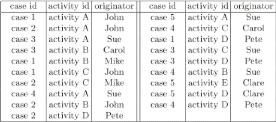
Table 1.1: An event log (audit trail).

Some event logs contain more information (more than the set of information shown in table (1.1)) on the case itself, i.e., data elements referring to properties of the case. They can logs every modification of some data element. Event logs are used as the beginning or starting point for mining.

1.3.2 Log filtering

The most potential next step for many applications after getting the events log is to filter it, i.e. to transform the log into another process log. Fundamentally, filtering a log is based on two basic actions : adding information to, or removing information from the process log.

There are different reasons why filtering is necessary. It is done for two main reasons: cleaning the data or narrowing down the analysis. Information systems are not free of errors and data may be recorded that does not reflect real activities. Errors can result from malfunctioning programs but also from user disruption or hardware failures that leads to erroneous records in the event log. Other errors can occur without incorrect processing. A log filter also can be considered as a function that transforms one process instance into another process instance, by adding or removing information. By filtering event logs, we obtain a process log that is easier to analyze or mine and less sensitive to noise.

The authors in [6] have defined log filtering as a function f where :

Let A be a set of activities and E be a set of event types, such that T ? (A × E) is a set of log events and W ? P(T^*) a process log over T. Furthermore, let A^' also be a set

17

Business Process and Process Mining

of activities and E^' also be a set of event types, such that T^' Ç (A^' x E^') is a set of log events. So f is defined as follow:

f : P(T^*) P(T^'*), i.e. a function that takes a trace as input and produces a different

trace as output.

1.3.3 Process Mining Perspectives

There are many important and interesting fields/perspectives for Process mining research, but three of them deserve special emphasis:

- Process perspective: Process perspectives focuses on the control-flow, i.e., tasks ordering. This perspective aims at finding a good characterization of all possible paths, e.g., expressed in terms of a Petri Net, an Event-driven Process Chain (EPC), or a UML activity diagram.

- Organizational perspective: Organizational perspective focuses on the originator field, i.e., which performers are involved and how are they related. This perspective aims at either to structure the organization by classifying people in terms of roles and organizational units or to show relations between individual performers (i.e., build a social network).

- Case perspective: Case perspective focuses on properties of cases. The cases paths in the process or their working originators can be used to characterize them. However, cases can also be characterized by the values of the corresponding data elements. For instance, if a case represents a replenishment order, it is interesting to know the supplier or the number of products ordered.

The above perspectives can be obtained as answers to the following kind of questions respectively:

· How? : can be used for the process perspective;

· Who? : can be used for the organizational perspective;

· What? : can be used for the case perspective.

18

Business Process and Process Mining

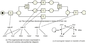
Figure 1.10: Some mining results for the process perspective (a) and organizational(b,c).

According to the authors [12, 50, 51], we can figure out three orthogonal aspects from the above perspectives:

1. Discovery of process knowledge like process models;

2. Conformance checking, i.e. measure the conformance between modeled behavior (defined process models) and observed behavior (process execution present in logs);

3. Extension, i.e., an a-priori model is enrich and extended with new aspects and perspective of an event log.

Process mining is mainly used to the discovery of process models. Therefore, much investigation has been performed in order to improve the produced models. However, many issues still complicate the discovery of comprehensible models and there is a need to consider them and provide solutions. The models generated tend to be very confusing and difficult to understand in case of processes with a lot of different cases and high diversity of behavior. These models are usually called spaghetti models [10].

1.3.4 Process Mining as Control-Flow Discovery

The term process discovery was introduced by Cook and Wolf [7], who apply it in the field of software engineering. They have proposed a Markov algorithm which can only discover sequential patterns. This is due to the fact that Markov chains cannot elegantly represent concurrent behavior. The idea of applying process discovery in the context of workflow management systems stems from Agrawal et al. [1].

19

Business Process and Process Mining

The value of process discovery for the general purpose of process mining [23] is well illustrated by the plugins within the ProM framework. It consists [53], of a large number of plugins for the analysis of event logs. The Conformance Checker plugin [29], for instance, allows identifying the discrepancies between an idealized process model and an event log. Moreover, with a model that accurately describes the event log, it becomes possible to use the time-information in an event log for the purpose of performance analysis, using, for instance, the Performance Analysis with Petri nets plugin.

Before investigating how some related works approaches are doing, we present bellow some basic notions:

· Invisible Tasks Refer to the type of invisible tasks that the technique can tackle. For instance, invisible tasks can be used to skip other tasks in a choice situation (see Figure 1.11(f), where B is skipped). Other invisible tasks are used for more elaborate routing constructs like split/join points in the model (see Figure 1.11(g), where the AND-split and AND-join are invisible "routing" tasks.).

· Duplicate Tasks Can be in sequence in a process model (see Figure 1.11(h)), or they can be in parallel branches of a process model (see Figure 1.11(i)).

· Non-free-choice Shows if the technique can mine non-free-choice constructs that can be detected by looking at local information at the log or non-local one. A non-local non-free-choice construct cannot be detected by only looking at the direct successors and predecessors (the local context) of a task in a log. The figures 1.11(c) and 1.11(d) both show a non-free-choice construct involving the tasks A, B, C, D and E. However, the Figure 1.11(d) illustrate a local non-free-choice, while the one in Figure 1.11(c) is not. Note that the task A never directly precedes the task C and a similar situation holds for the tasks B and D in any trace of a log for the model in Figure 1.11(c).

· Loops Points out if the technique can mine only block-structured loops, or can handle arbitrary types of loops. For instance, Figure 1.11(e) shows a loop that is not block-structured.

· Sequence, choice and parallelism Respectively show if the technique can mine tasks that are in a sequential, choice or concurrent control- flow pattern structure.

· The noise The event log contains rare and infrequent behavior not representative for the typical behavior of the process².

²Note that the definition of noise may be a bit counter-intuitive. Sometimes the term "noise" is used to refer to incorrectly logged events, i.e., errors that occurred while recording the events.

20

Business Process and Process Mining

· Incompleteness The event log contains too few events to be able to discover some of the underlying control-flow structures.

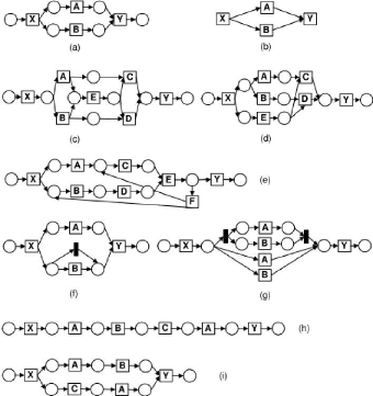
Figure 1.11: Illustration of the main control-flow patterns.

The remainder of this section describes the process discovery algorithms that have been applied in the context of Control-flow.

1.3.4.1 The á-algorithm

A well known process discovery algorithm that is based on the log relations is called the á-algorithm. Aalst et al.[35] have proved that á-algorithm can learn an important class of Workflow Nets, called Structured Workflow Nets, from complete event logs. The á-algorithm can be considered as a theoretical learner. In order to discover a Workflow Net from logs, it is necessary to establish the ordering between the transitions of this workflow. These relations will later be used in order to find places and connection between the transitions and these places. These relations, between two activities x and y are:

21

Business Process and Process Mining

· Direct succession x > y: x > y ? there are in log sub-traces...xy,

· Causality x -? y: x -? y ? x > y ?y x (i.e: if there are traces ...xy... and no traces ...yx...),

· Parallel x k y: x k y ? x > y ?y > x ( i.e. can be both ...xy... and ...yx...),

· Unrelated x#y: x#y ? x y ?y x (i.e. there are no traces ...xy... nor ...yx...). The set of all relations for a log L is called the footprint of L.

With these relations, the á-algorithm is defined as follows:

Algorithm 1 á-algorithm

Require: á(L) :

1: extract all transition names from L to set T

2: let TI be the set of all initial transitions and TO the set of all end transitions

3: find all pairs of sets (A, B) such that:

· tA ? A should be connected to all tB ? B via some place p,

· ?a ? A and ?b ? B holds a -? b,

· ?a1, a2 ? A: _a1#a2 and ?b1, b2 ? B: b1#b2.

4: once found all such sets, we retain only the maximal ones:

· a maximal set contains the maximal possible number of elements that can be connected via single place.

5: for each such pair (A, B), we connect all elements from A with all elements from B with one single place pA,B

6: then we also connect appropriate transitions with the input and output places.

7: finally we connect the start place j to all transitions from TI.

8: and all transitions from TO with the final state o.

Example of how á-algorithm works: Let us consider the log L=[abcd,acbd,aed]. Its footprint is:

	a	b	c	d	e
a	#	-?	-?	#	-?
b	?-	#	k	-?	#
c	?-	k	#	-?	#
d	#	?-	?-	#	?-
e	?-	#	#	-?	#

22

Business Process and Process Mining

· TI : the set of all first transitions in the log,

o in the table, for such transitions we don't have any incoming edges,

o i.e. it has only f- , no -? in its column,

o TI= {a}.

· T_o : the set of all last transitions in the log, o no outcoming edges, only incoming - in the rows,

o T_o= {d}

With this table, using -? and relations we can draw the following graph (a directed edge represents -? relation, undirected double edge represents relation):

With this graph we can enumerate the maximal sets A and B. Recall that for sets A and B :

· ?a1, a2 E A: a1#a2,

· ?b1, b2 E B: b1#b2,

· ?a1 E A, ?b1 E B : a1 -? b1.

	A		B	(1)
{a}	{b, e}		(2)
{a}	{c,e}		(3)
{b, e}	{d}		(4)
{c, e}	{d}

Note that b and c cannot belong to the same set( they are parallel).

Based on these sets:

· we add 4 places for each pair (A, B) to connect all elements from A with all elements from B with one place,

· and we add 2 more places: the start place j and the final state o.

23

Business Process and Process Mining

	A	B			p1
{a}	{b,e}
				p2
{a}	{c,e}
				p3
{b,e}	{d}
				p4
{c,e}	{d}

So we have:

The á-algorithm is remarkably simple, in the sense that it uses only the information in the ordering relations to generate a WF-Net. It assumes event logs to be complete with respect to all allowable binary sequences and assumes that the event log does not contain any noise. Therefore, the á-algorithm is sensitive to noise and incompleteness of event logs. Moreover, the original á-algorithm was incapable of discovering short loops or non-local, non-free choice constructs. Alves et al. [2] have extended the á-algorithm to mine short loops and called it á⁺-algorithm.

1.3.4.2 The á⁺-algorithm

Alves et al. [2], have introduced new ordering relations such as:

· a 4 b ? there is a subsequence ...aba... in the logs,

· ab ? there are sequences ...aba... and ...bab... And they have redefine the relations that cause the error:

· a -? b ? a > b ? (b a V ab), (this way we can correctly identify the follow relation when there's a loop of length 2)

24

Business Process and Process Mining

· a b ? a > b ? b > a ? no ab (by adding the last condition way we don't misidentify the parallel relation)

· therefore at this step we assume that the net is one-loop-free - i.e. it does not contain loops of length 1

· if it's not the case, we can turn our Worflow Net into one-loop-free by removing all transitions that create these loops.

Algorithm 2 á⁺-algorithm

Require: á⁺(W) :

1: let T be all transitions found in the log W

2: identify all one-loop transitions and put them into set L1L

3: let Ti be all non-one-loop transitions: Ti +- T - L1L

4: let _FL1L be the set of all arcs to transitions from L1L : it consists of:

· all transitions a that happen before t: a E Ti,s.t a > t,

· all transitions b that happen before t: b E Ti,s.t t > b,

5: now remove all occurrences of transitions t E L1L from the log W, let the result be

_W-L1L

6: run the á- algorithm on W-L1L

7: reconnect one-loop transitions back: add all transitions and from L1L and arcs from FL1L to transitions and arcs discovered by á

Wen et al. [52] made an extension for detecting implicit dependencies, for detecting non-local, non-free choice constructs. None of the algorithms can detect duplicate activities. The main reason why the á-algorithms are sensitive to noise, is that they does not take into account the frequency of binary sequences that occur in event logs. Weijters et al. [50] have developed a robust, heuristic-based method for process discovery, called heuristics miner.

1.3.4.3 The Heuristics algorithm

Heuristics Miner is a Process Mining algorithm that uses a statistical approach to mine the dependency relations among activities represented by logs. It focuses on the control flow perspective and generates a process model in the form of a Heuristics Net for the given event log. The formal approaches like the alpha algorithm i.e. an algorithm for mining event logs and producing a process model, presupposes that the mined log must be complete and there should not be any noise in the log. However, this is not practically

25

Business Process and Process Mining

possible. The heuristics miner algorithm was designed to make use of a frequency based metric and so it is less sensitive to noise and the incompleteness of logs.

The Heuristics Miner mines the control flow perspective of a process model. To do so, it only considers the order of the events within a case. In other words, the order of events among cases isn't important. For instance for the log in the log file only the fields case id, timestamp and activity are considered during the mining. The timestamp of an activity is used to calculate these orderings. The main difference with the á- algorithm is the usage of statistical measures (together with acceptance thresholds, parameters of the algorithm) for the determination of the presence of such relations.

The algorithm can be divided in three main phases: the identification of the graph of the dependencies among activities; the identification of the type of the split/join (each of them can be an AND or a XOR split); the identification of the "long distance dependencies". An example of measure calculated by the algorithm is the "dependency measure" that calculates the likelihood of a dependency between an activity a and b:

a == b = |a>b|-|b>a|

|a>b|+|b>a|+1, where:

· a > b indicates the number of times that the activity a is directly followed by b into the log.

Another measure is the "AND-measure" which is used to discriminate between AND and XOR splits:

a == (b ? c) = |b>c|+|c>b|

|a>b|+|a>c|+1^,

If two dependencies are observed, e.g. a -+ b and a -+ c, it is necessary to discriminate if a is and AND or a XOR split. The above formula is used for this purpose: if the resulting value is above a given threshold (parameter of the algorithm), then a is considered as an AND split, otherwise as XOR.

This algorithm can discover short loops, but it is not capable of detecting non-local, non-free choice as it does not consider non-local dependencies within an event log. Moreover, heuristics miner cannot detect duplicate activities. Alves de Medeiros et al.[36]) describe a genetic algorithm for process discovery.

1.3.4.4 The Genetic algorithm

Another approach to mine processes by mimicking the process of evolution in biological systems is called Genetic Mining. The main idea is that there is a search space that contains some solution point(s) to be found by the genetic algorithm. The algorithm starts by randomly distributing a finite number of points into this search space. Every point in the search space is called an individual and the finite set of points at a given

26

Business Process and Process Mining

moment in time is called a population. Every individual has an internal representation and the quality of an individual is evaluated by the fitness measure. The search continues in an iterative process that creates new individuals in the search space by recombining and/or mutating existing individuals of a given population.

A new generation is obtained at every new iteration of a Genetic algorithm. The parts that constitute the internal representation of individuals constitute the genetic material of a population. Genetic operators are used to perform recombination and/or modification of the genetic material of individuals. Usually, there are two types of genetic operators:

· Crossover: the crossover operator recombines two individuals (or two parents) in a population to create two new individuals (or two offsprings) for the next population (or generation),

· Mutation: the mutation operator randomly modifies parts of individuals in the population.

In both cases, there is a selection criterion to choose the individuals that may undergo crossover and/or mutation. To guarantee that good genetic material will not be lost, a number of the best individuals in a population (the elite) is usually directly copied to the next generation. The search proceeds with the creation of generations (or new populations) until certain stop criteria are met. For instance, it is common practice to set the maximum amount of generations (or new populations) that can be created during the search performed by the genetic algorithm, so that the search process ends even when no individual with maximal fitness is found [2].

The genetic miner is capable of detecting non-local patterns in the event log and is described to be fairly robust to noise. The goal of genetic mining is to get a heuristic net with the highest possible fitness, i.e. a net that best describes the log under consideration.

Aalst et al. [38] present a two-phases approach to process discovery that allows to configure when states or state transitions are considered to be similar. The ability to manipulate similarity is a good approach to deal with incomplete event logs. In particular, several criteria can be considered for defining similarity of behavior and states: the inclusion of future or past events, the maximum horizon, the activities that determine state, whether ordering matters, the activities that visibly can bring about state changes, etcetera. Using these criteria, a configurable finite state machine can be constructed from the event log. In a second phase, the finite state machine is folded into regions using the existing theory of regions [8].

27

Business Process and Process Mining

Schimm [31] has developed a mining tool suitable for discovering hierarchically structured workflow processes. This requires all splits and joins to be balanced. However, in contrast to other approaches, he tries to generate a complete and minimal model, i.e. the model can reproduce the log and there is no smaller model that can do so. Like Pinter et al. in [22], Schimm assumes that events either refer to the start or completion of an activity and he uses this information to detect explicit parallelism.

1.4 Evaluation metrics of Business Processes

In general, every scientific studies give rise to a new solutions and/or approaches. New solutions means new possibilities and opportunities, which led to an important problem: which is the best solution to adopt and how it is possible to compare the new solution against the others, already available in the literature?.

Evaluation of business processes and its involved elements is important as it is used as a tool to control and improve the processes. Different methods are used for this purpose which ranges from economics, statistics fields to computer science. In computer science, focus is to provide support in carrying out business operations (automation), storage (databases), computations (mining methods). Here, we focus on the evaluation of the computation aspect of business processes mining algorithm.

1.4.1 Performance of a Process Mining Algorithm

Since there is continually new process mining algorithms with different characteristics and factors which influence their performance, it is important to be able to select the best algorithms according different criteria. Performance of processes is measured in terms of performance indicators, e.g. throughput time. Process mining present ways to deal with these indicators.

1.4.2 Evaluating the discovered process

Many evaluation criteria can be used to measure the performance of an algorithm comparing to another. It depends on the aims of the use or the evaluation of the algorithm. In [54], the authors have adopted four main dimensions of quality criteria that can be used to specify different quality aspects of reconstructed process models: fitness, simplicity, precision and generalization.

28

Business Process and Process Mining

Fitness: the fitness aspect addresses the ability of a model to capture all the recorded behavior in the event log.

Precision: the precision points out if a process is overly general (a model that can generate many more sequences of activities with respect to the observations in the log). It requires that the model does not allow additional behavior very different from the behavior recorded in the event log.

Generalization: the generalization denotes if a model is overly precise. The discovered model should generalize the example behavior seen in the event log (a model that can produce only the sequence of activities observed in the log, with no variation allowed).

Simplicity: simplicity means that a process model is not exclusively restricted to display the eventually limited record of observed behavior in the event log but that it provides an abstraction and generalizes from individual process instances.

The above dimensions can be used to identify the aspects highlighted in a model. For instance, in (Figure 1.12) four processes are displayed with different levels for the different evaluation dimensions. Suppose, as reference model, the one in (Figure 1.12 (a)), and assume that a log it can generate is presented in Table (1.2).

1207	ABDEI
145	ACDGHFI
56	ACGDHFI
28	ACHDFI
23	ACDHFI

Table 1.2: Example of log traces, generated from the executions of the process presented in (Figure 1.12 (a)).

In (Figure 1.12 (b)), the concerned process is called "flower model". It allows any possible sequence of activities and, essentially, does not define an order among them. For this reason it has very low precision, even if it has high fitness, generalization and structure.

The process (Figure 1.12 (c)) is just the most frequent sequence observed in the log, so it has medium precision and high structure but low fitness and generalization. In (Figure 1.12 (d)) the process is a "complete" model, where all the possible observed behaviors in the log can be reproduce without any flexibility. This model has high fitness and precision but low generalization and structure.

29

Business Process and Process Mining

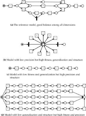
Figure 1.12: Four process where different dimensions are pointed out (inspired by Fig. 2 of [28]). The (a) model represents the original process, that generates the log of Table 2.2; in this case all the dimensions are correctly highlighted; (b) is a model with a low fitness; (c) has low precision and (d) has low generalization and structure.

In the remaining part of the section some metrics are presented. In particular, it is possible to distinguish between metrics model-to-log, that compare a model with a log and metrics model-to-model that compare two models.

1.4.2.1 Model-to-log Metrics

Using Process Mining techniques, these metrics aim at comparing log with the process model that has been derived.

According to [54], these metrics can be grouped in three main categories as follow :

30

Business Process and Process Mining

1- Metrics to quantify fitness

Fitness considers also the "problems" happened during replay (e.g. missing or remaining tokens in a Petri Net) so that actions that can't be activated are punished as the action that remains active in an improper way [29].

Completeness very close to the Fitness, takes into account trace frequency as weights when the log is replayed [36].

Parsing Measure is defined as the number of correct parsed traces divided by the number of traces in the event log [21].

2- Metrics to quantify precision/generalization

Soundness calculates the percentage of traces that can be generated by a model and are in a log (so, the log should contain all the possible traces) [10].

Behavioral Appropriateness evaluates how much behavior is allowed by the model but is never used in the log of observed executions [29].

ETC Precision evaluates the precision by counting the number of times that the model deviates from the log (by considering the possible "escaping edges") [11].

3- Metrics to quantify structure

Structural Appropriateness measures if a model is less compact than the necessary, so extra alternative duplicated tasks (or redundant and hidden tasks) are punished [29].

1.4.2.2 Model-to-model Metrics

Unlike the first category of metrics, Model-to-model Metrics aim at comparing two models, one against the other. Authors in [9] have enumerated four types of metrics:

Structural Similarity Aims at measuring the "graph edit distance" that is the minimum number of graph edit operations (e.g. node deletion or insertion, node substitution, and edge deletion or insertion) that are necessary to get from one graph to the other [9].

31

Business Process and Process Mining

Label Matching Similarity Is based on a pairwise comparison of node labels: an optimal mapping equivalence between the nodes is calculated and the score is the sum of all label similarity of matched pairs of nodes [9].

Dependency Difference Metric Counts the number of edge discrepancies between two dependency graph (binary tuple of nodes and edges) [5],

Process Similarity (High-level Change Operations) Counts the changes required to transform a process into another one, with 'high level' changes (not adding or removing edges, but 'adding activity between two', and so on).

1.5 Conclusion

In this chapter we have introduced a different techniques of process mining. Recall that the aim of process discovery is to aid a process designer in improving the support for a process by an information system. Hence, it heavily depends on the specific information that can be taken from an information system, which process discovery approach best suits the designer.

In this chapter we presented again different approaches for the evaluation of process models, in particular a model-to-model and a model-to-log metric. For most of this techniques, good tool support is essential, such as ProM.

32

Chapter2

Process Mining Tools

2.1 Introduction

Process mining is a process management technique that allows for the analysis of business processes based on event logs. The basic idea is to extract knowledge from event logs recorded by an information system. Process mining aims at improving this by providing techniques and tools for discovering process, control, data, organizational, and social structures from event logs. Without these techniques it is difficult to obtain a valuable information.

Many free and commercial software's framework for the use and implementation of process mining algorithms have been developed. In this chapter we will focuses on the ProM framework which is largely used because of its extensibility and the fact that it supports a wide variety of process mining techniques in the form of plug-ins.

This chapter is devoted to the presentation of the ProM framework. First we gives an overview on what consist log filtering and how to do some basic log filtering orations in ProM. Then we present some mining plug-ins, which are implementation of different mining algorithms. After that, we shows that it is possible to get much more information's by applying some analysis techniques on the mining results. And then, we present another very important kind of plug-ins which provide to ProM the ability to convert one model into another model. Finally we ends this chapter by a short conclusion.

2.2 ProM Architecture

The (Pro)cess (M)ining framework (ProM) is an extensible framework that supports a wide variety of process mining techniques in the form of plug-ins. It is an independent

33

Process Mining Tools

platform as it is implemented in Java. It was developed as a framework for process mining but now it becomes much more versatile, currently including many analysis and conversion algorithms, as well as import and export functionality for many formalisms, such as EPCs and Petri Nets. Figure 2.1 presents an overview of the ProM Framework architecture, it shows the relations between the framework, the plug-ins and the event log.

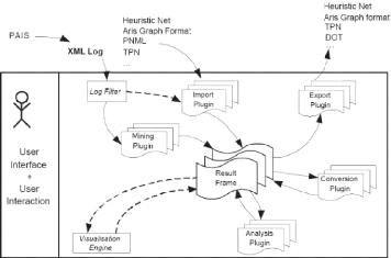
Figure 2.1: Overview of the ProM Framework. (adapted from [41])

As shown in Figure 2.1, the event logs are generated by Process-aware Information Systems (PAIS) [12]. To read an event logs, ProM framework uses the Log Filter, and it can also perform some filtering tasks to those logs before performing any other task. As (Figure 2.1) shows, the ProM framework allows to use five different types of plug-ins:

· Import plug-ins: This king of plug-ins are used to load a wide variety of models.

· Mining plug-ins: Many different mining algorithms are implemented in this kind of plug-ins, e.g., mining algorithms that construct a Petri Net based on some event log.

· Analysis plug-ins: This family of plug-ins implement some property analysis on some mining result. For instance, for Petri Nets there is a technique which constructs place invariants, transition invariants, and a cover ability graph.

· Conversion plug-ins: The main offered functionality by these plug-ins is the ability to transform the mining results into another format, e.g., from BPMN to Petri Nets.

34

Process Mining Tools

· Export plug-ins: Export plug-ins are used as final step. They offer and implement some "save as" functionality for some objects (such as graphs). For instance, there are plug-ins to save EPCs, Petri Nets... etc.

2.3 Log Filters

We have seen in section 1.3.2, that the concept of a log filter refers to a function that typically transforms one process instance into another process instance. Many of log filters have been developed. In the rest of this section, we discuss and introduce on what consist a log filter and how filters are applied to a log.

Filtering logs is a procedure by which a log is made easier to analyze and typically less sensitive to noise. This is done by using different kind of options. For instance, in ProM, the option "keep" is used to keep all tasks of a certain event (Figure 2.2), also, the option "remove" allows to omit the tasks with a certain event type from a trace, and the option "discard instance" allows to discard all traces with a certain event type.

Figure 2.2: Log filter Screenshot (In ProM).

In ProM options can be selected by clicking on an event type. The Start Events filters the log so that only the traces (or cases) that start with the indicated tasks are kept. The End Events works in a similar way, but the filtering is done with respect to the final tasks in the log trace. The Event filter is used to set which events to keep in the log.

Filtering logs, and instead of removing information, allows to add information. For instance, if assumption is made that all cases start and end with the same log event, a log filter could add an initial event, and end event to each instance of a valid assumption.

35

Process Mining Tools

2.3.1 Adding artificial 'start' and 'end' events

Figure 2.3 shows the obtained process model for a call center example, using the Fuzzy Miner.

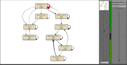
Figure 2.3: Process model using the Fuzzy Miner on a non filtered event log.

As we can see in the obtained process model, it is not easy at all to see where the process starts and where it ends. There is no clear beginning or end point because all of the activities are connected. To create a clear start and end point in a process models, we can use the so-called " Adding artificial 'start' and 'end' events" in ProM6.

The figure 2.4, shows the obtained process model after filtering the event log used in the process model of the figure 2.3.

36

Process Mining Tools

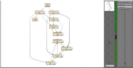
Figure 2.4: Process model after filtering the event log

Now, the main path of the process is clearly visible. Most process instances are handled by an incoming call at the front line and are then directly completed.

Example 2 (Adding End events) : The Figure 2.5 illustrate the result of generating a model using the heuristic miner. It is clearly visible that there is two 'End' events.

Figure 2.5: Process model using the heuristic miner before filtering.

To create only one clear end point in the process model, In ProM 6, we can use the so-called "Add End Artificial Events". By doing this, when discovering a process model based on the filtered log, we get the following process model (Figure 2.6):

37

Process Mining Tools

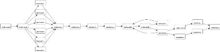
Figure 2.6: Process model using the heuristic miner after filtering.

2.3.2 Duplicate Task filter

In an event log, it can happen that two events are directly repeated with the same name. Duplicate Task filter (Figure 2.7) allows to remove such a direct repetitions.

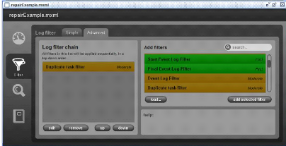
Figure 2.7: Duplicate Task filter.

2.3.3 Remove attributes with empty value

Another important feature in ProM is the ability to remove all the attributes with an empty value (Figure 2.8). This provide the advantage to keep only events that have a certain attribute value. But it does not always work reliably, so it is recommended to make sure to check the effect of the filter in the Inspector.

38

Process Mining Tools

Figure 2.8: Removing attributes with empty value.

2.3.4 Enhanced Event Log filter

Frequency also can be used as a basic parameter in log filtering (Figure 2.9). Events and process instances can be filtered based on an activity-based frequency percentage threshold. This is particularly useful if there are hundreds of different events to, for instance, focus only on activities that occur in most of the cases.

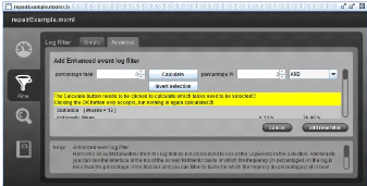
Figure 2.9: Enhanced Event Log filter.

39

Process Mining Tools

2.3.5 Time based log filter

Another technique to log filtering is by using time as a basic parameter. The time-based log filter technique uses the timestamp to filter: traces by duration or traces by starting time (as shown in Figure 2.10).

Figure 2.10: Time based log filter.

2.4 Mining Tools

Different types of process mining tools are available, each with their own strengths and weaknesses. Mining tools are an implementation of mining algorithms. Tools like ProM offer an easy way to use the different mining techniques. Some of the control-flow discovery tools include a plenty of plug-ins.

2.4.1 á-algorithm plug-in

It implements the á-algorithm [30], which proceed by constructing a Petri Net that models the workflow of the process (Figure 2.11). By assuming that the log is complete (all possible behavior is present), the algorithm establishes a set of relations between tasks. The main limitations of the á-algorithm are: it is not robust to noise and it cannot mine processes with short-loops or duplicate tasks. Several works have been done to extend this algorithm and to provide solutions for its limitations like the work in [48], in which, the authors have proposed an extension in order to be able to mine short-loops.

40

Process Mining Tools

Figure 2.11: alpha miner.

2.4.2 Tshinghua-á-algorithm plug-in

Which uses timestamps in the log files to construct a Petri Net (Figure 2.12). It is related to the á-algorithm, but uses a different approach. Details can be found in [51].

Figure 2.12: Tshinghua alpha miner.

2.4.3 Heuristics miner plug-in

In this plug-in [50], the Heuristics miner algorithm extend the alpha algorithm by considering the frequency of traces in the log. It can deal with noise, by only expressing the main behavior present in a log. To do so, it only considers the order of the events within a case. In other words, the order of events among cases isn't important.

41

Process Mining Tools

The figure 2.13, illustrate the result of using the heuristic miner algorithm (In ProM framework) on the log example illustrated in the table 2.1.

ID	Process Instance	Frequency
1	ABCD	1
2	ACBD	1
3	AED	1

Table 2.1: Example of an event log with 3 process instances, for the process of patient care in a hospital (A: Register patient, B: Contact family doctor, C: Treat patient, D: Give prescription to the patient, E: Discharge patient)

Figure 2.13: Process Model of the example log

2.4.4 Genetic algorithm plug-in

It uses genetic algorithms to calculate the best possible process model for a log. A fitness measure that evaluates how well the individual can reproduce the behavior present in the input log is assigned to every individual. In this context, individuals are possible process models. Candidate individuals are generated using genetic operators like crossover and mutation and then the fittest are selected. This algorithm was proposed to deal with some issues involving the logs, like noise and incompleteness [36].

To illustrate what kind of graph is presented by this tool, we used the example show in table 2.1, and used the ProM implementation of this algorithm to come to the result shown in Figure: 2.14

42

Process Mining Tools

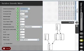
Figure 2.14: Process Model of the example log with genetic miner.

Some of the organizational perspective tools available in ProM that approach this subject are:

2.4.5 Social Network miner plug-in

This plug-in reads a process log and generates social networks (Figure 2.15) that can be used as a starting point for SNA (Social Network Analysis). Several techniques can be applied to analyze the social networks, e.g., find interaction patterns, evaluate the role of an individual in an organization, etc. The main idea of the social network miner is to monitor how individual process instances are routed between actors. It exist five kinds of metrics to generate social networks, They are 'handover of work', 'subcontracting', 'working together', 'similar task', and 'reassignment' (for more information see [37]).

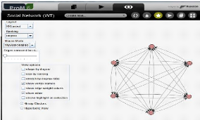
Figure 2.15: Descovering social networks by ProM.

43

Process Mining Tools

2.4.6 Organizational Miner plug-in

Organizational mining focuses on the organizational perspectives such as organizational models. It works at a higher level of abstraction than the previous techniques. While the Social Network Miner works at the level of the individual, the Organizational Miner technique works at the level of teams, groups or departments.

2.4.7 Staff Assignment Miner plug-in

Staff assignment mining aims at defining who is allowed to do which tasks. Its techniques mine and compare the 'real' staff assignment rules with the staff assignment rules defined for the underlying process afterwards. Based on this comparison, possible deviations between existing and mined staff assignment rules can be automatically detected [25].

There are other kind of mining tools which deal with the data perspective and which use not only the information about activities and events, but they also make use of additional data attributes present in logs. An example of such miners is the Decision Miner.

2.4.8 Decision Miner plug-in

Decision Miner analyzes how data attributes of process instances or activities (such as timestamps or performance indicators) influence the routing of a process instance. To do so, the Decision Miner analyzes every decision point in the process model and if possible links it to the properties of individual cases (process instances) or activities [4].

There are also some plug-ins that deal with less structured processes:

2.4.9 Fuzzy Miner plug-in

The process models of less structured processes, tend to be very confusing and hard to read (usually referred to as spaghetti models). This tool aims to emphasize graphically the most relevant behavior, by calculating the relevance of activities and their relations (see Figure2.3). To achieve this, two metrics are used [40]:

1. Significance: Measures the level of interest to an events (for example by calculating their frequency on the log),

2. Correlation Determines how closely related two events that follow each other are, so that events highly related can be aggregated.

44

Process Mining Tools

In the context of process mining, using a mining plug-in on a log to obtain a model of some sort is typically the first stage. But, it may be not sufficient. The resulting model may need some additional analysis or needs to be converted into another format. For this purpose, ProM contains analysis and conversion plug-ins, as shown in the remainder of this Chapter.

2.5 Analysis Tools

Even if process mining is very concluding step, the resulted process models still typically static structures that compactly describe information that was generated from the log. These models however are not the final result. Instead, there may be more interesting results by answering questions about the obtained results, i.e there may be questions that can only be answered by analyzing the results of mining in a larger context. It exist analysis plug-ins that serve this purpose, i.e. they take a number of models or other structures as input and then perform analysis techniques that relate to the question under investigation. Next we present only a few of those that we consider more relevant:

2.5.1 Conformance checker

Conformance checker [29] analyzes the gap between a model and the real world, detecting violations (bad executions of a process) and ensuring transparency (the model might be outdated). The conformance checker supports analysis of the (1) Fitness, (2) Precision (or Behavioral Appropriateness), and (3) Structure (or Structural Appropriateness) dimension( as show in Section 1.4.1.

Fitness The token-based fitness measure f relates the amount of missing tokens with the amount of consumed ones and the amount of remaining tokens with the amount of produced ones. If the log can be replayed correctly, i.e., there were no tokens missing nor remaining, it evaluates to 1. If every produced and consumed token is remaining or missing the metric evaluates to 0 (Figure 2.16). There are several options to enhance the visualization of the process model (Token Counter, Failed Tasks, Remaining Tasks, Path Coverage, Passed Edges).

45

Process Mining Tools

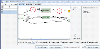
Figure 2.16: Model view shows places in the model where problems occurred during the log replay.

Behavioral Appropriateness Behavioral appropriateness consist on analyzing if the process model allow or not for more behavior than that recorded in the log (Figure 2.17). This "extra behavior" detection is also called precision dimension, i.e., the precision is 100% if the model "precisely" allows for the behavior observed in the log. This way can, for instance, to discover alternative branches that were never used when executing the process.

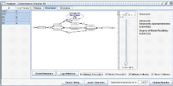
Figure 2.17: Analysis of the precision of a model allows to detect overgeneral parts.

Structural Appropriateness Structure is the syntactic ways by which behavior (i.e., the semantics) can be specified, using the vocabulary of the modeling language (for example, routing nodes such as AND or XOR) in a process model (Figure 2.18). However, it is not the only way, there are several other syntactic ways to express the same behavior, and there may be "preferred" and "less suitable" representations. Clearly, it highly depends on the formalism of the process modeling and is difficult

46

Process Mining Tools

to assess in an objective way. However, it is possible to formulate and evaluate certain "design guidelines", such as calling for a minimal number of duplicate tasks in the model.

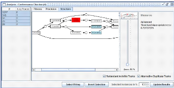
Figure 2.18: Structural analysis detects duplicate task that list alternative behavior and redundant tasks.

2.5.2 Woflan plug-in ( A Petri-net-based Workflow Analyzer)

Woflan (WOrkFLow ANalyzer) [42], analysis a Petri Nets based definitions of workflow process (Figure 2.19). It has been designed to analyze the correctness of a workflow. Woflan it consists of three main parts: parser, analysis routines, user interface.

Figure 2.19: The correctness of a model using Woflan tool.

2.5.3 Performance analysis

Drives performance information about a process using the timestamps stored in logs and a Petri Net. After that, the performance data is visually represented in the form of a

47

Process Mining Tools

Petri Net (Figure 2.20).

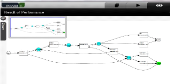
Figure 2.20: Scheenshot of the analysis plug-in Performance Analysis with Petri net.

2.5.4 LTL checker

Checks whether a log satisfies some Linear Temporal Logic (LTL) formula (Figure 2.21). For instance, it can check if a given activity is executed by the person that should be executing it or check activities ordering, like, whether an activity A that has to be executed after B are indeed always executed following the right order [41].

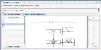
Figure 2.21: Scheenshot of the analysis plug-in LTL Checker Plugin (Example raining) [41]

In this section, we have presented several analysis plug-ins for different purposes. The overview given in this section is far from exhaustive. Although many analysis techniques have been developed for specific purposes. We have seen that ProM allows the user to use many more analysis techniques. It has a particular power which is the fact that formalisms can be converted back and forward using conversion plug-ins.

48

Process Mining Tools

2.6 Conversion Plug-ins

To translate of one formalism into another, ProM provides some conversion plug-ins. So, with ProM it is really easy to convert one model into another model if one is willing to accept some loss of information or precision.

2.6.1 BPMN to Petri-Net

The BPMN to Petri-Net translation is implemented in the context of ProM as a plug-in named 'BPMN to Petri Net conversion plug-in'. Translations from BPMN to Petri Nets can be very useful because they are applicable in most practical cases. The figure 2.23 shows the result of the conversion of the BPMN illustrated in Figure 2.22.

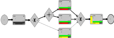
Figure 2.22: BPMN example

The Figure 2.23 shows a labelled Petri Net, where the transitions relating to functions are labelled with the function labels and the transitions relating to connectors are labelled with ô and shown in black. Furthermore, in the background, the conversion plug-in used a special set of reduction rules to remove as many of those ô-labelled transitions as possible, without changing the behaviour. However, the resulting Petri Net still shows a lot of ô-labelled transitions. These transitions correspond to the OR-split and the OR-join.

49

Process Mining Tools

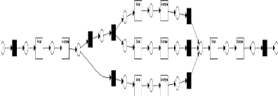
Figure 2.23: Petri net translation of the BPMN in Figure 2.22

2.6.2 Petri Net to Yawl Model

The figure 2.24 shows a YAWL model as a result from converting the Petri Net. In this case, the conversion plug-in is able to remove all routers (i.e., the invisible transitions) from the resulting process model. Removing the invisible transitions introduces an OR-join and an OR-split, moreover conditions (corresponding to Petri Net places) are only introduced when needed. Clearly, such as smart translation is far from trivial.

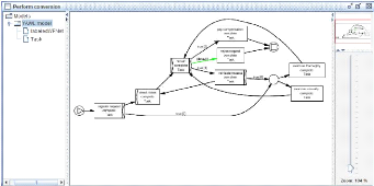
Figure 2.24: The mined review process model converted to a YAWL model.

2.6.3 Petri Net into WF-Net

It is also possible to convert Petri Net into WF-Net. There is a specific plug-in for that (Petri net into WF-net plug-in). In the case a Petri Net contains multiple source places, then a new source places will be added. Also, for every old source place a transition will be added that can move the token from the new source place to the old one [40].

50

Process Mining Tools

2.6.4 YAWL model into EPC

An other conversion plug-in serves to convert YAWL models into EPC (YAWLToEPC). It follows the following steps:

1. Find the root decomposition of the YAWL model,

2. Convert every ordinary YAWL condition into a chain of two EPC (XOR) connectors. The first connector will be a join, the second a split,

3. Converts every YAWL input condition into a chain of a start EPC event, a dummy EPC function, and an EPC (XOR-split) connector,

4. Converts every YAWL output condition into a chain of an EPC (XOR-join) connector and a final EPC event,

5. Converts every YAWL task into a chain of an EPC (join) connector, a dummy EPC event, an EPC function, and an EPC (split) connector. The type of both connectors depends on the input/output behavior of the YAWL task. If the YAWL task refers to another YAWL decomposition, this decomposition is converted as well (steps 2 to 6), although no start or end events (see steps 3 and 4) will be generated for this decomposition.

6. Converts every YAWL edge into a corresponding EPC edge,

7. Reduces as many EPC connectors as possible,

8. Removes any source/sink EPC connectors.

It exist many other conversion plug-ins for ProM framework, such as: Petri Net to Heuristic Net, Petri Net to Epc,...etc. This characteristic makes ProM one of the most useful tool for process mining.

51

Process Mining Tools

2.7 Conclusion

In this chapter we have introduced some important concepts related to process mining tools. We have presented the main characteristics and plug-ins of one of the most popular mining framework, which is ProM. We have seen that ProM is very useful and provides several advantages. The continuous growth of ProM is due to the importance that process mining has gained in recent years, resulting in numerous research performed by people around the world.

The next chapter will be devoted to the comparison between different mining techniques following different criteria.

52

Chapter3

Comparison and analysis of process

mining algorithms

3.1 Introduction

There are many process mining algorithms with different theoretical foundations and aims, raising the question of how to choose the best for a particular situation. This is a problem, for both, businesses using process mining and for researchers evaluating new developments. There is a need for methods for objectively comparing process mining algorithms against known characteristics of business process models and logs, in terms of what can be re-discovered and how much data is required to do so.

In the previous chapters we have seen different concepts related to business process and process mining, different evaluation criteria and metrics and then we have presented some process mining tools.

In this chapter we use the ProM framework (presented in chapter 2) to objectively analyze and compare process mining algorithms against a known ground truth. The analysis in this chapter concerns three mining algorithms, namely: the Alpha algorithm, Heuristic algorithm and Genetic algorithm, according to the metrics presented in the chapter 1.

3.2 Problem Description

We have seen that it exists a plenty of approaches and paradigms to process mining. There are approaches with local methods which look at local relations between activities

53

Comparison and analysis of process mining algorithms

in logs ( á, á⁺, Heuristics Miner), and global approaches which build and refine a model based on the whole log (Genetic Mining, Fuzzy Miner [40]).

In general, each algorithm has its one specialisms, e.g. the Heuristics Miner uses frequencies and parametrization to handle noise, á- algorithm is able to mine models that adhere to the restrictions of Structured Workflow Nets (SWF-nets) [35], but not mine implicit dependencies or handle noisy logs well and Genetic miner can mine complex and noisy logs, but it is resource intensive.

In some considerations, having a plenty of algorithms can be see as advantage, as it offers many use possibilities, but from another point of view, it also constitutes a problem of making the choice which algorithm to use. There is a need for a method to objectively compare process mining algorithms, to enable informed choice of which to use in a situation. Which algorithms work "best", in what circumstances? Which results are the "best", and can this be quantified in terms of accuracy or confidence [27].

3.3 Comparison and analysis

For the experimentation and to make comparison between the three algorithms (Alpha, Genetic and Heuristic), we have chosen to use an existing real-life event log. In this section we will run different tests on events log using the ProM framework. For each test, one small log file is mined with one algorithm and the resulted process model (converted, and) exported as a Petri Net. Next, we run the Conformance Checker plug-in [29] to measure the mined model against the underlying process described by event logs. The collected results can then be analyzed. Data recorded include each algorithm's specific reports, such as the characteristics of the discovered Petri Net, plus the Conformance Checker's assessment of the model's Fitness, Behavioral Appropriateness (under-fitting) and Structural Appropriateness (over-fitting and generalization), Structural precision (and recall) and Behavioral precision (and recall).

3.3.1 Log description

We have chosen two main event logs for the experimentation and comparison task. The first one was provided in the Fourth International Business Process Intelligence Challenge (BPIC'14) as a challenge for the participants, to analyze its data using whatever techniques available. It reflect an activity undertaken by the Rabobank Group ICT (Rabobank Nederland) and it contains a log of the activity of the various incidents that may arise during the change of new software releases.

54

Comparison and analysis of process mining algorithms

The processes within Rabobank ICT 3.1 revolve around the following service desk processes: Interaction Management, Incident Management, Change Management.

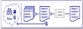
Figure 3.1: The processes within Rabobank ICT

The Table 3.1 shows an extract of the event log that we use :

DateStamp	Incident-Activity-Number	Incident-Activity-Type	Assignment-Group	KM-number
07/01/2013 08:17	001A3689763	Reassignment	TEAM0001	KM0000553
04/11/2013 13:41	001A5852941	Reassignment	TEAM0002	KM0000553
04/11/2013 13:41	001A5852943	Update from customer	TEAM0002	KM0000553
04/11/2013 12:09	001A5849980	Operator Update	TEAM0003	KM0000553
04/11/2013 12:09	001A5849978	Assignment	TEAM0003	KM0000553
04/11/2013 12:09	001A5849979	Assignment	TEAM0002	KM0000553
04/11/2013 12:09	001A5852942	Closed	TEAM0003	KM0000553
04/11/2013 12:09	001A5852172	Caused By CI	TEAM0003	KM0000553
04/11/2013 12:09	001A5852173	Reassignment	TEAM0003	KM0000553
25/09/2013 08:27	001A5544096	Operator Update	TEAM0003	KM0000553
03/06/2013 11:15	001A4725475	Update	TEAM9999	KM0000611

Table 3.1: Extract of the event log

The second event log is provided in the chapter 5 in [35], it contains instances of some reimbursement process. The table 3.2 shows a fragment of the log corresponding to the handling of requests for compensation. Each line presents one event. The events are already grouped per case. Case 1 has five associated events. The first event of Case 1 is the execution of activity register request by Pete on December 30th, 2010. There is different properties attributes for each event, like date and timestamp, ressource or cost.

55

Comparison and analysis of process mining algorithms

Case id	Event id	Timestamp	Activity	Resource	Cost
1	35654423	30-12-2010:11.02	Register request	Pete	50
	35654424	31-12-2010:10.06	Examine thoroughly	Sue	400
	35654425	05-01-2011:15.12	Check ticket	Mike	100
	35654426	06-01-2011:11.18	Decide	Sara	200
	35654427	07-01-2011:14.24	Reject request	Pete	200
2	35654483	30-12-2010:11.32	Register request	Mike	50
	35654485	30-12-2010:12.12	Check ticket	Mike	100
	35654487	30-12-2010:14.16	Examine casually	Pete	400
	35654488	05-01-2011:11.22	Decide	Sara	200
	35654489	08-01-2011:12.05	Pay compensation	Ellen	200
3	35654521	30-12-2010:14.32	Register request	Pete	50
	35654522	30-12-2010:15.06	Examine casually	Mike	400
	35654524	30-12-2010:16.34	Check ticket	Ellen	100
	35654525	06-01-2011:09.18	Decide	Sara	200
	35654526	06-01-2011:12.18	Reinitiate request	Sara	200
	35654527	06-01-2011:13.06	Examine thoroughly	Sean	400
	35654530	08-01-2011:11.43	Check ticket	Pete	100
	35654531	09-01-2011:09.55	Decide	Sara	200
	35654533	15-01-2011:10.45	Pay compensation	Ellen	200

Table 3.2: A fragment of the second event log: each line corresponds to an event.

3.3.2 Experimentation

This part is devoted to do some experimentation's to compare results of using different algorithms for process mining. To do that, we have used a real-life event loge, which reflect an activity undertaken by the Rabobank Group ICT (Rabobank Nederland) and reimbursement. Mining was carried out using the á-Miner, Heuristics Miner (HM), Genetic Miner (GM) algorithms, using the ProM framework. We have chosen these three algorithms because they are fundamental algorithms, commonly used, implemented in the ProM framework, and represent significantly different approaches to process mining. We perform experimentation according to different kind of metrics, which are:

1. Fitness

2. Precision and Generality

3. Precision and Recall

On bellow, we expose the obtained results for each metric.

3.3.2.1 Fitness

To calculate the fitness, we have used the event logs with different traces number. We start by 10 traces and we increase the number by 2 traces for each time, until 28 traces.

56

Comparison and analysis of process mining algorithms

We have experimented the three algorithms, mentioned above, under two scenarios: at first we used the file as it is, and the second scenario is after being filtered using the plug-in filter "filter log using simple heuristics (see section 2.3). Figure 3.2 shows the results (In the form of a graph) before filtering.

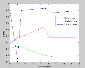
Figure 3.2: Fitness against the number of traces before filtering

We can see in the figure 3.2 that the Heuristic Miner recorded a slight growth in the fitness against a number of traces equal to 12, after that, it began to decline and then stabilize around 0.2 fitness against a number of traces higher than 22. This result for the Heuristic Miner, can be interpreted by the fact that the event logs contain a lot of noise, and that this algorithm takes into account the frequent traces which is not the case with this log file (most traces are not frequent).

Also for the alpha algorithm, the graph begins with a growth in the fitness values against a number of traces in the interval [10, 19], but it recorded a sharp fall thereafter, and stabilizes on the value 0.5 for fitness, against a number of traces higher than 21. The result of Alpha Miner can be interpreted by the fact â€â€that this algorithm does not take into account the noise, it only considers the relationships between activities.

The last algorithm, which is the Genetic Miner, begins directly with a decrease but grows after 12 traces and stabilizes around 0.9 for fitness with a slight increase after a number greater than 20 traces. This can be interpreted by the fact that Genetic Miner do not only uses the method of Heuristic Miner to consider noise, but also duplicate tasks.

57

Comparison and analysis of process mining algorithms

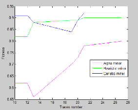
Figure 3.3: Fitness against the number of traces after filtering

The figure 3.3 shows the obtained results after filtering events logs. It is clearly visible that there is a marked improvement for the three algorithms. We can see that both algorithms Genetic Miner and Alpha miner, after a slight decline, they recorded growth when the number of traces is higher than 13 traces and they stabilize around 0.9 and 0.8 for fitness, respectively. Concerning the Heuristic miner algorithm, the graph is growing and stabilizes at 0.9 fitness when the number of traces is higher than 21. So after filtering, the best results are achieved by Heuristic Miner and Genetic Miner algorithms. This can be explained by the fact that the filter is used to filter and keep only the events that we want and that are relevant, which contribute to obtain much more similar traces. It is also worth to note that the best value of the fitness is registered by the Genetic Miner algorithm.

3.3.2.2 Precision and Generality

Precision and generality are very common and important aspects of comparison between models in many fields of research in computer science. Researchers are still trying to find a good compromise between these capital characteristics. Due to their nature, it is important to find a good balance between both.

In process discovery, precision and generality are a major challenge. Although models should be precise, generalizing beyond observed behavior is also a necessity. So process discovery algorithms should be able to balance between underfitting(overly general models) and overfitting (overly precise models). Therefore, superior precision and generality

58

Comparison and analysis of process mining algorithms

metrics should be at hand.

There are two kinds of measures which can be used to quantify precision and generality: Behavioral Appropriateness and Structural Appropriateness.

Behavioral Appropriateness

Behavioral Appropriateness consist on analysis and detection of "Extrat behavior" of the model. A Process model may allow for more behavior than that recorded in the log. There is two metrics for this measure :

· Simple behavioral appropriateness: (see section 2.5.1): measure saB based on the mean number of enabled transitions during log replay (the greater the value the less behavior is allowed by the process model and the more precisely the behavior observed in the log is captured). Note that this metric should only be used as a comparative means for models without alternative duplicate tasks.

· Advanced Behavioral Appropriateness: aaB allows to compare the behavior that is specified by the model with the behavior that is actually needed to describe the behavior in the event log. Therefore, this metric makes use of an analysis of "follows" and "precedes" relations, both in the model and the event log. Comparing the variability of these relations allows the definition of a precision metric that penalizes extra behavior.

Structural Appropriateness

In a process model, there are several syntactic ways to express the same behavior. Structure is the syntactic means by which behavior can be specified, using the vocabulary of the modeling language. Therefore, having several ways implies different characteristics which may be "preferred" (for example, easier to understand) and "less suitable" representations. To quantify the degree of structural appropriateness, the only currently available model-log metrics are:

· Simple Structural appropriateness: saS is a simple measure based on the size of the graph (the greater the value the more compact is the model). Note that this metric should only be used as a comparative means for models allowing for the same amount of behavior.

· Advanced structural appropriateness : aaS is a generality metric that evaluates two specific design guidelines for expressing behavioral patterns. This measure

Comparison and analysis of process mining algorithms

will punish for both alternative duplicate tasks and redundant invisible tasks. Note that these guidelines are definitely not the only behavioral preferences of control-flow models. However, aaS is the only metric that quantifies generality in some way. Ideally, a process model does not contain redundant invisible tasks nor alternative duplicate tasks. Accordingly, this measure will punish for models that simply enumerate all traces in the event log and for models that entail too much irrelevant invisible tasks.

In this part we investigate the above metrics. For that, we use two examples from real-life datasets (The first one contains instances of some reimbursement process (We took the file used in the chapter 5 in [35]) and the second file contains the detail incident activity of the Rabobank ICT (which we already used for measuring fitness)). Short names are used in the first dataset: a = register request, b = examine thoroughly, c = examine casually, d = check ticket, e = decide, f = reinitiate request, g = pay compensation, and h = reject request.

The Figures (3.4, 3.5, 3.6) show the obtained models according to the used algorithms (Alpha, Genetic and Heuristic respectively).

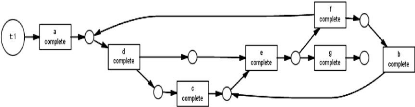
Figure 3.4: Mined model by Alpha algorithm

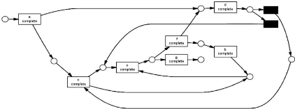
59

Figure 3.5: Mined model by Genetic algorithm

Comparison and analysis of process mining algorithms

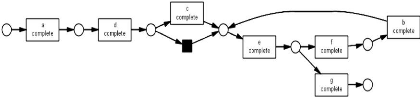
Figure 3.6: Mined model by Heuristic miner

The table 3.3 shows the metrics values for the first example. We note that both Alpha and Heuristic algorithms provide the same and a good structural appropriateness, while Genetic produce models with a poor structural appropriateness.

On the other hand, Alpha and Heuristic algorithm produces a model with reasonable behavioral appropriateness, while Genetic algorithm produce model with excellent behavioral appropriateness.

	Alpha	Heuristic	Genetic
Structural Appropriateness	0.6	0.6	0.15
Behavioral Appropriateness	0.8	0.8	0.97

Table 3.3: Conformance checker between the first example and its mined models

In the second example, we have considered one trace with the ID = IM0047050 from the incident detail activity (the firs event log) dataset. The figures (3.7, 3.8, 3.9) show the obtained models after using three algorithms.

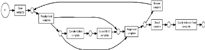
60

Figure 3.7: Mined model by Alpha algorithm case 2

61

Comparison and analysis of process mining algorithms

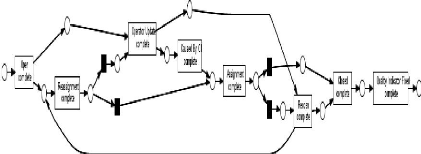
Figure 3.8: Mined model by Genetic algorithm case 2

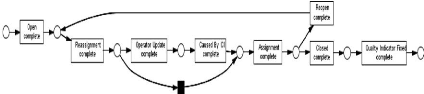
Figure 3.9: Mined model by Heuristic miner case 2

The table 3.4 shows that Alpha and Heuristic algorithms produce models with excellent behavioral appropriateness. While Genetic algorithm produces a model with reasonably good structural similarity. All of three algorithms produce models with excellent structural appropriateness.

	Alpha	Heuristic	Genetic
Structural Appropriateness	1	1	1
Behavioral Appropriateness	0.95	0.94	0.79

Table 3.4: Conformance checker between IM0047050 case and its mined models

The above two examples (based on real-life datasets) have illustrated that different process mining algorithms perform differently on different models. As a result, researchers need to benchmark different process mining algorithms to select appropriate algorithms for their models, but this can be computationally expensive and take a long time.

3.3.2.3 Precision and Recall

Precision and Recall are the basic measures used in evaluating search strategies. In the first case, we are interested in two metrics, which are the structural precision and the

Comparison and analysis of process mining algorithms

structural recall. In the second case we are interested in the behavioral precision and the behavioral recall.

Structural precision and recall: Structural precision and structural recall are based on the causality relations of the mined and original models, and were adapted from the precision and recall metrics presented in [22]. These metrics basically work by checking how many causality relations the mined and the original model have in common. The more causality relations the two models have in common, the more similar their structures are. The structural precision assesses how many causality relations the mined model has that are not in the original model. The structural recall works the other way around. Note that the structural similarity performed by these metrics does not consider the semantics of the split/join points[3].

Behavioral precision and recall: Behavioral precision and behavioral recall are based on the parsing of an event log by the mined model and by the original model. The behavioral precision checks how much behavior is allowed by the mined model that is not by the original model. The behavioral recall checks for the opposite. Additionally, both metrics take into account how often a trace occurs in the log [3].

To test these metrics we used the example of instances of some reimbursement process used in the book [35]. We took the original model with 8 different events logs. In the following, we present the obtained results.

The figure 3.10 illustrate the obtained results for precision.

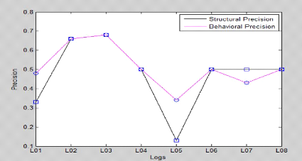
Figure 3.10: Average Structural precision and Behavioral precision values

62

63

Comparison and analysis of process mining algorithms

The figure 3.11 illustrate the obtained results for recall.

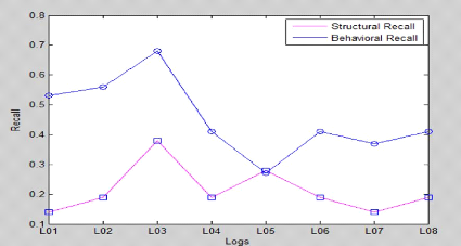
Figure 3.11: Average Structural recall and Behavioral recall values

All these four metrics are complementary when assessing the quality of a mined model. Moreover, the application of these metrics is not limited to the evaluation of the different algorithms. They can be applied to another settings where models need to be compared.

3.4 Conclusion

In this section we have presented the seven metrics that are used to analyze the results of the experiments: the fitness, precision and generalization, the behavioral precision (BP), the behavioral recall (BR),the structural precision (SP) and the structural recall (SR). The fitness addresses the ability of a model to capture all the recorded behavior in the event log. Precision and generalization enables the user to control the balance between "overfitting" and "underfitting". The BP and BR measures how precise the mined model is. The SP and SR express if the mined model has an overly complex structure or not. These metrics are complementary and should be considered together during the experiments analysis.

64

Chapter4

Proposition

4.1 Introduction

Process discovery aims to reconstruct process models from execution logs. Specifically: given a log, each of the cases (i.e. execution traces) is analyzed, eventually producing a (Petri net) model of the process. Existing techniques perform well on structured processes, but still have problems discovering and visualizing less structured ones. In reality, there is a lot of diversity leading to complex models that are difficult to interpret. Trace clustering is one of very promising technique to best mining results. Trace clustering approach aims at splitting the event log into homogeneous subsets and for each subset a process model is created.

The aims of our work in this chapter is to provide a solution that will improve traces clustering compared to the existing techniques. We rely on the work already proposed by Song et al [32], where we define another distance measure between two cases. Our contribution is the use of Boolean logic through the »XOR» and »AND» function to calculate the distance between two traces and new clusters centres.

4.2 Proposition description

For well-structured processes, e.g. workflows, the discovery aspect of process mining has limited appeal, since it is bound to confirm the prescribed characteristics of the process. There are, however inherent problems of applying process mining to flexible environments. Since these environments typically allow for a wide spectrum of potential behavior, the analysis results are equally unstructured. The typical problems observed in resulting process models are an overwhelming number of task nodes, and equally large

65

Proposition

numbers of relations, resulting in the stereotypical "spaghetti models". One dominant factor contributing to unstructured mining results is diversity of an event log, i.e. single cases differ significantly from one another. It is, in such cases, a valid assumption that there are a number of tacit process variants hidden within one event log, each significantly more structured than the complete process.

The problem with diversity, i.e. that a set of cases are structured very differently, obviously grows with the number of cases being analyzed. Thus, one solution to this problem is to reduce the number of cases which are analyzed at once. Tacit processes will usually not be explicitly known, i.e. there is no available knowledge on how to partition the set of cases. One can, however measure the similarity of cases and use this information to divide the set of cases into more homogeneous subsets. The authors in Song et al [32]. have got the idea to use the conventional clustering methods. They were the first who applied the methods of clustering in the mining process field, such that (K-means, Quality Threshold, agglomerative Hierarchical Self-Organizing Map (SOM)).

Autors in[32] points correspond to cases, i.e., process instances that left a trace in the log, each case is characterized by a defined set of items, i.e., specific features which can be extracted from the corresponding trace. Items for comparing traces are organized in trace profiles, each addressing a specific perspective of the log. Based on a set of profiles, each measuring a number of features for each case from a specific perspective. Based on these feature matrices, a number of distance metrics can be applied to compute the relative distance between any two cases in the log. To check the accuracy of the generated model, we can perform a conformance check. In [26] two types of metrics are proposed: (1) fitness and (2) appropriateness.

For our proposition to trace clustering, we built our approach using a part of the work of Song et al.[32] by adopting their definition of traces profiles but with different distance measure and cluster center calculation. We define another way to calculate the distance between one case and a cluster center, we use the Boolean logical "XOR" to calculate the distance between two points and the AND logical operator to calculate new centers of the clusters. The figure 4.1 shows the main steps in our traces clustering approach.

66

Proposition

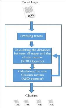
Figure 4.1: Our clustering approach overview

4.2.1 Trace Profiles

In the authors [32] approach case is characterized by a defined set of items, i.e., specific features which can be extracted from the corresponding trace. Items for comparing traces are organized in trace profiles, each addressing a specific perspective of the log.

Every clustering algorithm attempts to group sets of similar points, whereas for trace clustering, the points to be clustered are log traces. Thus, in order to cluster traces in a meaningful way, we first have to establish what makes two traces similar. Event logs in the MXML format contain a large amount of structured information. Some of this information is explicit (e.g., names of events), however there is also derived information, e.g. the number of events within a trace.

wIn our approach, traces are characterized by profiles, where a profile is a vector Profile_V ector composed of n items (hich support binary values) as follow :

Profile_Vectori = (a1, a2, ..., a_n).

67

Proposition

Where _aj=1..n are binary values representing if an activity aj is present in the trace or not. 1 means the activity occur at least once, and 0 means that the activity does not occur in the trace. These resulting vectors will be used to calculate the distance between traces and to calculate the clusters centers. A cluster center is represented also by a Trace profile.

4.2.2 XOR Operator

The XOR function, often called eXclusive OR or exclusive disjunction is a logical operator of Boolean algebra. The inputs to a binary XOR operation can only be 0 or 1 and the result can only be 0 or 1.

This operator is used in electronics, computer science, and also in cryptography because of its interesting properties. It will always produce a 1 output if either of its inputs is 1 and will produce a 0 output if both of its inputs are 0 or 1.

We use XOR, because as it is an "exclusive OR", it only returns a "true" value (1) if the two values are exclusive, i.e. they are both different. So, applying XOR between two profiles will provide us a serie of 1 for each two different items of the vectors profiles. This will serve as a mean to calculate the difference degree of tow profiles.

If we consider two traces profiles A and B and their vector items, the Table 4.1 shows the fourth possibles case when applying XOR between the binary values of the profiles vectors and their meanings.

Item (Activity)	Ai	Bj	Ai XOR Bj	interpretation for our approach
1	0	0	0	the two traces have no occurrence of the activity (The traces are similar concerning the activity 1).
2	0	1	1	one of the two traces have at least one occurrence of the activity (The traces are mutually exclusive concerning the activity 2
3	1	0	1	one of the two traces have at least one occurrence of the activity (The traces are mutually exclusive concerning the activity 3
4	1	1	0	the two traces have at less one occurrence of the activity (The traces are similar concerning the activity 4).

Table 4.1: Interpretation of XOR results

4.2.3 AND Operator

The Logical AND is an operator on two logical values that produces a value of true if and only if both of its operands are true. We apply the logical AND on the values of two

68

Proposition

Traces profiles among all the traces in the same cluster to built a new cluster center. The table 4.2 show how we use the logical AND between two items of a ProfileV ector.

Item (Activity)	Ai	Bj	Ai AND Bj	interpretation for our approach
1	0	0	0	the two traces have nothing in common concerning the activity 1.
2	0	1	0	the two traces have nothing in common concerning the activity 2.
3	1	0	0	the two traces have nothing in common concerning the activity 3.
4	1	1	1	the two traces have occurrences of the activity 4, so they can be considered similar.

Table 4.2: Interpretation of AND results

The process of applying the logical AND among a set of traces profiles provide at the end a vector in with all the items at 1 represent the activities which occur in all the traces in the set.

4.2.4 Clustering Algorithm

As used in the [32], we use the K-means clustering algorithm, because it is the most commonly used in practice among partitioning methods, which constructs k clusters by dividing the data into k groups. The steps below, illustrate the main steps in our clustering approach.

1. Define a profile for each case x (1 if the activity exists, 0 otherwise);

2. Define one or more centers (the center is defined as a kind of filter (ie: define the activities we want to see in each cluster (1 if there's an activity we wish to see, otherwise 0);

3. Calculate the distance between each point (each case) and each center (the distance is defined as an XOR operator);

4. Based on the distance, gather all traces that have a minimum distance from to the center or centers;

5. Calculate the new center for each cluster (which is defined as a LOGICAL AND between all traces in the same cluster);

6. Repeat step (3 to 5), until we have a stable cluster configuration;

7. For each cluster, verify the distance of each point from to the cluster, remove the distance exceeds 2.

69

Proposition

4.2.4.1 Distance Measure

To calculate the distance between a trace and each clusters we use the XOR operator as follow:

let consider a traces profile a, and cluster center profile b : a = (0001111) and

b = (1101011)

We have a XOR b = (1100100)

To calculate the distance between a and b, we use this measure (D) = the sum of the resulted vector item :

D = 1 + 1 + 0 + 0 + 1 + 0 + 0 = 3

The value 3 can be seen as the degree of difference between the trace a and the cluster center b. In our approach, we add a trace to the cluster with the minimum distance among the distances to all the clusters centers. This can be interpreted as follow : we add the trace to the cluster which represent a minimum differences with the trace.

4.2.4.2 Calculate new clusters

In our approach, new clusters are built by applying logical AND between traces in the same cluster. For instance, having two traces a = (0001111) and c = (1101011) in the same cluster, the new cluster ci will be :

ci = (0001011)

This can be interpreted as follow : we obtain a new cluster center profile, in which, each item having the value 1 means that the corresponding activity is occurred at least once in all the traces of the cluster.

4.3 Running Examples

In this section we will apply our approach (Which we have implemented using Java language) on different event logs and we will compare obtained results against these of the approach of the Song et al [32], which is already implemented in ProM 5.2.

The first event log (Shown in Table 4.3) we use is that one used by song et al [32]. Each row refers to a single case and is represented as a sequence of events. Events are represented by the case identifier (denoted by the row, e.g., 1), activity identifier (first element, e.g., A), and originator (second element, e.g., John).

70

Proposition

Case ID	log events
1	(A,John),(B,Mike),(D,Sue),(E,Pete),(F,Mike),(G,Jane),(I,Sue)
2	(A,John),(B,Fred),(C,John),(D,Clare),(E,Robert),(G,Mona),(I,Clare)
3	(A,John),(B,Pete),(D,Sue),(E,Mike),(F,Pete),(G,Jane),(I,Sue)
4	(A,John),(C,John),(B,Fred),(D,Clare),(H,Clare),(I,Clare)
5	(A,John),(C,John),(B,Robert),(D,Clare),(E,Fred),(G,Robert),(I,Clare)
6	(A,John),(B,Mike),(D,Sue),(H,Sue),(I,Sue)

Table 4.3: Example process logs (A: Receive a item and repair request, B: Check the item,

C: Check the warranty, D: Notify the customer, E: Repair the item, F: Test the repaired product, G: Issue payment, H: Send the cancellation letter, I: Return the item)

Table 4.4 shows the result of profiling the example log from table 4.3. Each row of the table corresponds to the profile vector of one trace in the log. The Trace profile defines one item per type of activity (i.e., event name) found in the log. Measuring an activity item is performed by simply counting if the activity has at least one occurrence in the trace.

Case ID	Trace Profile
	A	B	C	D	E	F	G	H	I
1	1	1	0	1	1	1	1	0	1
2	1	1	1	1	1	0	1	0	1
3	1	1	0	1	1	1	1	0	1
4	1	1	1	1	0	0	0	1	1
5	1	1	1	1	1	0	1	1	0
6	1	1	0	1	0	0	0	1	1

Table 4.4: traces profiles for the example log from 4.3

The table 4.5 shows the metrics measures concerning the obtained clusters for both approaches. At first, we have executed it for K = 2 (K represent the number of clusters) (song et al. approach and our approach respectively). We see that we got a slightly better fitness.

	Song et al		Our Approach
	Cluster 1	Cluster 2	Cluster 1	Cluster 2
Traces	( T1,T3)	(T2, T4, T5, T6)	(T1, T2, T3)	(T1, T6)
Fitness	1	0.89	0.96	1.00
behavioral appropriateness	1	0.91	0.97	0.96
structural appropriateness	0.6	0.66	0.55	0.57

Table 4.5: Metrics values

Also for k = 3, we have practically the same results for the cluster 1 and cluster 2 but we have a better fitness for the cluster 3. The metrics values are shown in the table ( 4.6).

Proposition

		Song et al						Our Approach
	Cluster (T3,T1)	1	Cluster (T5, T2)	2	Cluster (T4, T6)	3	Cluster (T3,T1)	1	Cluster (T2,T5)	2	Cluster (T4)	3
Fitness	1		0.87		0.91		1		0.87		1
behavioral appropriateness	1		0.96		0.90		0.96		0.95		1.00
structural appropriateness	0.6		0.66		0.50		0.6		0.66		0.60

Table 4.6: Metrics values

The second event log we use is already proposed by [41], which contains instances of some reimbursement process. We apply the two approaches, that of Song et al and ours. The event logs contains 1391 cases, as illustrated in table 4.7.

Traces	Frequencies
acdeh	480
abdeg	210
adceh	200
abdeh	170
acdeg	130
adceg	95
adbeh	61
adbeg	45

Table 4.7: Event logs form [39]

For k = 2, we got a better fitness and appropriateness for the metrics values (Table 4.9).

	Song et al		Our Approach
	Cluster 1	Cluster 2	Cluster 1	Cluster 2
Fitness	0.90	0.89	0.99	0.99
behavioral appropriateness	0.80	0.70	0.89	0.90
structural appropriateness	0.50	0.49	0.64	0.56

Table 4.8: Metrics values for the second event log

Also for k = 3, we have again better fitness for the all clusters. The metrics values are shown in the table (4.9).

	Song et al			Our Approach
	Cluster 1	Cluster 2	Cluster 3	Cluster 1	Cluster 2	Cluster 3
Fitness	0.94	0.93	0.96	1	1	0.99
behavioral appropriateness	0.80	0.90	0.86	0.90	0.95	0.92
structural appropriateness	0.56	0.60	0.50	0.61	0.64	0.60

71

Table 4.9: Metrics values

72

Proposition

Once we compare the model with respect to the event log, we come to compare the model with respect to another model. For this we take the latest example as shown in table (Table 4.7).

We take the original model, and we compare the obtained models by our approach and Song and al. For this we use Heuristic miner for modeling and structural precision/recall, behavioral precision/recall for calculating similarity between two models. We get the following results :

	Song et al			Our Approach
	Cluster 1	Cluster 2	Cluster 3	Cluster 1	Cluster 2	Cluster 3
behavioral precision	0.97	0.72	0.70	0.83	0.97	0.89
behavioral recall	0.90	0.57	0.85	0.77	0.90	0.81
structural precision	1.00	0.90	0.80	1.00	1.00	1.00
structural recall	0.70	0.52	0.50	0.50	0.64	0.64

Table 4.10: Metrics values

As shown in the table (4.10), we also have a better accuracy than Song et al. This reflects that the obtained traces by our approach in each cluster are much similar to each other.

4.4 Discussion

As shown in the results illustrated by the different tables in this section, we obtain a slight improvement results with respect to these of the song et al approach. Moreover, our approach is different from the approach of Song at several levels which can contribute to the reduction of the number of the Algorithm iterations and the time of execution. Below, we show the main differences :

1. The consideration of a single parameter in the clustering process, which is activities. In Song et al [32] approach, they consider activities and originators.

2. In Song and al approach, the filter must be done before clustering, in our approach, the filtering is done at the time of the construction of clusters (filtering and construction of clusters are at the same time)

The major drawback of our approach, is in the fact that it does not take into account the loops.

73

Proposition

4.5 Conclusion

Since trace clustering operates on the event log level, it can be used to improve the results of any process mining algorithm. In this chapter we have presented our methodology for trace clustering, which can effectively resolve diversity-related problems, by dividing the log into smaller, more homogeneous subsets of traces. We have used the concept of trace profile introduced by Song et al [32]. which is suitable way for characterizing and comparing traces. Based on trace profile, we have proposed a new way to calculate the distance between two cases and a new way to construct new clusters. The obtained results are slightly different to those obtained by song et al [32] with less complicated clustering algorithm.

74