Financial development and economic growth in Rwanda

2.3 Co nclusio

The chapter examined three theoretical views about the link between economic growth and financial development: the one stating that the financial sector development leads to economic growth, another putting economic growth ahead of financial development and lastly the view which does not support the importance of financial development on economic growth. On the empirical side, a strong positive role of financial development on economic growth has been found mostly in developed countries, and a weak or absence of link in developing countries. In some cases, the demand leading hypothesis has not been supported. In the next chapter we present the Rwandan financial sector.

Financial Development and Economic Growth in Rwanda

CHAPTER 3

OVERVIEW OF THE RWANDAN FINANCIAL SECTOR 3.0 Introduction

This chapter narrows the financial development issue to Rwandan case and highlights the weaknesses as well as the strength of the Rwandan financial system. To situate the level of financial development in macroeconomic perspective, a brief review of Rwandan economy is first presented. The chapter finishes with a comparison of the financial sector in Rwanda with those of other country members of East African region where Rwanda and Burundi were admitted in 2008.

3.1. Overview over the Rwandan economy

Rwanda is a small landlocked country in Central-East Africa, with 26,338 square kilometers. Its GDP per capita was $ 62.95 in 1970 with a population of 3.7 million, eight years after its independence from Belgium in 1962. The country is hampered by mountainous terrain and distance from the sea.

Rwanda is among most densely populated countries in Africa. In 2009, Rwanda was ranked 29^th among densely countries in 239 countries with density of 379 people per square kilometer, far ahead of the African average of 34 people per square kilometer. In 2009, the population was 9.998 million, growing at 2.8 %, compared to African average of 1.66 %, thus putting increasing pressure on agriculture land and environment (United Nations Population Division, 2008).

Rwanda's economy is essentially rural; nearly 81% of the population lives in rural areas (United Nations Statistic Division, 2009) and derives its livelihood from subsistence agriculture, cultivating coffee and tea for export with rudiment methods. Besides agriculture, there is exploitation of scarce natural resources in some regions like cassiterite, wolframite, and methane recently discovered in Lake Kivu.

Rwandan economy has been improving since 2000 with an increasing growth
rate especially for the last four years, when the country maintained an average

growth rate vis-à- vis many African countries over the period 2005-2008. In fact, the growth rate was 7.2 % in 2005, 7.3% in 2006, 7.9 % and 11.2 % in 2007 and 2008 respectively accumulating into an average growth rate of 8.4 % above the African average rate of 5.82% during this period. In addition, the country became the third, after Angola and Ethiopia (IMF, 2009). Moreover, Rwanda has made considerable efforts in improving living conditions of her population. Poverty has fallen by 3%, from 60% of the population living under the poverty line in 2000/2001 to 56.9% in 2006 but leaving 37.9% still extremely poor (IFAD website). However, Rwanda's development indicators are still below the African and East African averages, as indicated by the table below:

Table1: Trends i n average of per capita GDP

Indicator	Country	1970= 1980	1981= 1990	1991= 2000	2000= 2008		Overall average	Per capita GDP (in US$)
Rwanda	147.4	323.5	268.2	276.6	250
	489.21	768.9	733.9	1029.8	734.59
	232.45	313.9	278.8	346.76	288.69		Growth rate of GDP (%)
Rwanda	5.54	2	3.2	7.13	4.36
	3.08	3.26	3.17	5.27	3.55
	3.87	2.14	2.82	5.83	3.5		Share of Gross capital formation in GDP (in %)
Rwanda	14.45	18.71	13.35	17.27	15.84
	29.80	26.07	20.05	24.26	25.32
	22.29	17.77	16.26	19.15	18.94

Source: Author's calculations from data provided by United Nations Statistics Division, CIA World Fact books and World Development indicators Database.

As the table indicates, for the period 1981-1990 Rwanda reached the highest average per capita GDP with $323.5 compared to the average of $276.6 during the recent period ranging from 2000-2008. In addition, it is only in this period where its per capita GDP and the share of Gross capital formation in GDP was

above East African average. This was mainly due to political stability and favorable weather that prevailed during that time which made agricultural sector to contribute a lot in GDP.

The period 1990-2000 was marked by war of four years (1990-1994), the genocide of 1994 in which more than one million lost their lives and insecurity which affected the north (1996-1998). This explains the decrease in above indicators. Despite this situation, the growth rate of GDP exceeded African and East African average, as the country was trying to recover. Although the recent period was marked by the highest per capita GDP in 2008 with $ 458.49, but the period was characterized by a low per capita GDP in the period ranging from 2001-2003, a figure less than $200.

It is worth to say that it is in 2008 where the country recovered and passed over the level of per capita GDP reached before the genocide, that of 1988 with $360.87. The per capita GDP has been declining as from 1989, one year before the beginning of the war of 1990, up to 1994 from $360.87 in 1988 to $207.43 in 1994. Since 1995, the economic growth started to recover and currently, though the per capita GDP is still low, but Rwanda is among top performing in Africa with the growth rate currently above both African and East African average.

Many reasons explain the poverty of the country: being a landlocked country, on this it added the bad governance which has characterized the country since its independence, war, genocide and insecurity, lack of natural resources, little skilled human capital, as per year 2005, less than 1% of the population had a tertiary education, and a low level of investment.

3.2 The Rwandan financial sector

We analyse the financial sector by looking at the banking sector, MFIs, insurance companies and financial markets. We begin by mentioning that the Rwandan financial sector can be traced back from the creation of the Central Bank, National Bank of Rwanda and issue of the local currency, Rwandan Franc (RWF) in April 1964.

Financial Development and Economic Growth in Rwanda

3.2.1 Banking sector

The development of the financial sector before the genocide of 1994 was slow. At the time, only 3 commercial banks and 2 specialized banks operated with a total of less than 20 branches in the country, and one microfinance (UBPR) with around 146 branches. The war and the genocide affected heavily the banking sector: The genocide itself resulted in closure of the Central bank for 4 months. The former government left the country in 1994 for the DRC, after committing the genocide, with two-thirds of the national monetary base in addition to US $7 million in cash which was taken from the UBPR (Alson et al, 2001). Consequently, it took two years for this bank to reopen, in 1996. Moreover, almost both physical and human capital of all banks were destroyed during the genocide.

The post genocide period was marked by increase in number of banks, where in 2002 there were 6 commercial banks with 28 branches, 2 specialized banks and 1 union of financial institutions (UBPR) with 148 branches (NBR, 2004). In 2007, commercial banks operated only 38 branches, making only 7 % of all branches of financial institutions and by the end of 2008, 8 commercial banks, 2 specialized banks and 1 Microfinance bank were operating.

However, there was a lack of competition as three banks (BCR, BK and ECOBANK) held 66% market share before the licensing of UBPR as commercial bank in 2008. This situation has led to high interest rate spreads (8.6% in 2005), a modest 16% per annum growth in deposits over the past 5 years, and lending primarily to a core group of about 50 relatively large customers concentrated in Kigali and a few sectors (Murgatroyd et al, 2007).

The penetration of banking sector is very low, and worse in rural areas. The survey conducted by FinMark Trust in 2008 showed that in general, only 14 percent of the active population use banks, 7% use MFIs, 26% are informally served and 52% are financially excluded. In rural areas, less than 6 percent of the population hold savings account in a formal finance institution. Indeed, penetration of domestic credit to the private sector is underperforming, with 11

Financial Development and Economic Growth in Rwanda

percent of GDP, compared to 18 percent of GDP for peer countries (NBR, 2008).

Several reasons explain the underdevelopment of financial services. The weak culture of savings among the people is due to low level of per capita income in the country. In fact, in 2009 Rwanda was ranked 21^st poorest of the least developed countries in the world and 56.9 percent of its population lives on less than US$0.45 equivalent a day, the poverty threshold in Rwanda (IMF, 2009).

Secondly, a high spread between the deposit rate (around 7%) and a lending rate (around 16%) does not provide an incentive to the public to save. Many bank accounts are used as a payment mechanism for employees. It is important to note that due to relative higher penetration of UBPR, it has been upgraded to commercial bank in 2008 and became BPR S.A, and that KCB, a new regional bank from Kenya has been licensed.

3.2.2 Microfi na nce institutions

Microfinance initiatives mushroomed from 2002, primarily as a response to the weak involvement of the traditional banks in small and micro enterprises, and rural areas. Sixty-three microfinance institutions were licensed in 2006 (Habyalimana, 2007).

In 2009, the microfinance sub-sector consisted of around 125 MFIs including 111 COOPECS (Kantengwa, 2009). In June 2006, NBR estimated that MFIs represented 24.18% of the total financing of the economy with RWF 59bn (equivalent of $100 million) out of RWF 244bn of credit of the financial institutions and 25% of savings mobilization. The mobilized savings amounted to RWF 65bn (equivalent to around $.110 million) out of RWF 259bn. Informal finance is so popular that 73 % of total population reported using informal loans in 2005 (Habyalimana, 2007).

However, Microfinance institutions are inexperienced, characterised by management with poor corporate governance, weak information systems, important losses caused by poor internal organisation and a mismanagement of their loan portfolio (Kantengwa, 2009). All these weaknesses culminated into

the failure of nine microfinance institutions in 2006 with total deposits of more than $5.3 million, leading to a general panic (NBR, 2007). To include rural population in the financial system, UMURENGE SACCOs was introduced in the end of 2008, a saving scheme to be operating in each of 421 sectors.

3.2.3 Insurance and pension funds

This sector comprises 5 classic insurance companies (SONARWA, SORAS, COGEAR, CORAR and Phoenix of Rwanda Assurance Company) and six insurance brokers. In 2006, only about 3% of the active population held insurance policy. In addition, there are three public medical insurance companies: RAMA, MMI and Mutuelle de Santé and one private company, AAR Health Services, licensed in 2008. The relatively well performing RAMA and MMI serve only 5% of the population (NISR, 2008).

The pension sector is assured by one Public Pension fund (SSFR) and 10 Growing Private Pension funds. The SSFR covers only 7.5% of active population and on overall less than 8% of the active population is under pension schemes (NBR, 2009).

3.2.4 Financial markets

In January 2008, Rwanda established a capital market with the creation of an Over-The-Counter market operated and regulated by a Capital Market Advisory Council (CMAC). However, its market capitalisation is still very low as only $ 360, 000 has been traded in 15 transactions (the average of $24,000 in each transaction) and newspapers frequently reported that the OTC has been silent due to lack of transactions recorded. The main reason is the poverty of Rwandan citizen which does not allow the culture of saving where even those who earn monthly salary are able to spend it for survival only. With regard to market participants, Rwandan OTC has 7 members divided into three categories: Stockbrokers, Dealers and Sponsors (CMAC website).

3.2.5 Financial liberalization i n Rwanda

Before the financial liberalization, tools of monetary policy were mainly credit
rationing, directed credit and interest rate controls. The financial deregulation

was characterized by legal reforms affecting the nature of central bank supervision and new tools of monetary policy were introduced like regal reserve requirements and discount rate, alongside the abolition of interest rate ceilings, directed credit and credit rationing as well.

The process of financial liberalization started in March 1995 by the liberalization of exchange rate and interest rate in 1996. In the same year, banking structure was opened to foreign investment and entry requirements for MFIs were relaxed. However, despite abolition of controls on interest rates, the rigidity in the later is still observed, fluctuating around 16% for lending and 7% for deposit rates of interest, due to oligopolistic nature of the banking system.

The period 2004-2006 was characterized by take over of nonperforming banks due to poor corporate governance. BACAR and BCDI were taken over by FINABANK and ECOBANK respectively, and the government sold its majority of share in BCR. In 2006, the spread of MFIs nationwide came as another step in financial liberalization, following the failure of commercial banks to deliver in rural areas. However, as prophesized by Diaz-Alejandro (1985), the end of 2006 and 2007 turned the financial sector in crisis as consequence of unmonitored regularization, after which the central bank started exerting basic controls on financial institutions through micro finance law and regulation adopted in 2008, and strengthened by creation of MFI association created in 2007.

3.2.6 Monetary policy i n Rwanda

Monetary policy is a responsibility of the NBR and is a part of the annual economic program aiming at implementing the medium-term program referred to as EDPRS. Like all central banks, NBR uses open market operations, reserve requirements (fixed at 8% before 2009 and reduced to 5% from 2009), and discount rate (which fluctuates between 7.5 % and 8%). With its basic objective of price and foreign exchange stability, its development can be regarded in two periods: the period of financial regulation, from 1964 to 1995 and after liberalization in 1995.

Before 1995, the country was in fixed exchange rate regime. From 1970 to 1990, the foreign exchange rate was 1$ for nearly 82 RWF. However, the war period 1990-1994 saw many devaluations, especially that of 1991 with 51.5 % and that of 1994 of 91.64% and by the end of 1994, the exchange rate stood at 1$ for 220 RWF (DUSHIMUMUKIZA, 2006).

The period of flexible exchange rate was characterized by volatility in exchange rate. As evidence, in January 2003, the average exchange rate stood at 511.2168 RWF for 1$, but by end of the year, the exchange rate was at 574.83RWF for 1$. The depreciation rate stood at 11.6% from one year to another. If we compare the average exchange rate of 2002 and 2008, the index is 115.2 in six years, from the exchange rate of 475.32 FRW for 1$ in 2002 to 547.61 FRW for 1$ in 2008 (NBR, annual report, 2008). Indeed, this exchange rate can be compared to 220 RWF for 1$ in 1994.

Regarding price stability, again the rampant inflation characterized the after liberalization period, as compared to the period before where the price stability was observed. Evidence from Kigali (the Capital city) in 2003 shows that the CPI for all products in constant terms of 1982 was 559.32 compared to the CPI of 408.93 and in 1996 (NBR, annual report of 2003). The inflation rate is fluctuating around 7.5%

For money supply, there was an upward trend in money supply to the level where its growth rate was above that of GDP. For instance, in 2007, increase in money supply was 31.25% against 13% of nominal GDP. Indeed, in some years, the money supply experiences an over expansion, especially during election periods like 2003 and 2008.

For payment system monetization, SIMTEL was introduced in 2005 aiming at speeding up the level of financial innovation, which is very low, as in 2008 the value of transactions using bank cards was 0.59 percent of the non cash payment instruments (dominated by cheques) and cash payment represented 98% of the payment system (NBR, 2009). Introduction of Real Time Gross Settlement and an Automated Clearing House were few among mechanisms of such modernization.

Financial Development and Economic Growth in Rwanda

3.3 Comparison of financial development within EAC

The discussion omits comparison based on the number of financial institutions as the countries are not equally sized and formal financial markets since Rwanda and Burundi do not have them while Kenya launched its stock market (Nairobi Stock Exchange) in 1954 and those of Tanzania and Uganda are operational since 1998. We rather use some ratios regarded as proxies of the level of financial development.

The need for this comparison lies in the sense that the macroeconomic policies of these countries are tied together, hence it pays for Rwanda to know its status quo in this community of countries. Three indicators are used: Liquid liabilities as % of GDP, claims on private sector to GDP ratio and domestic credit to GDP ratio. Data which are sources of the figures are presented in appendices.

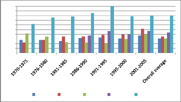
3.3.1 Ratio of Liquid liabilities (M3) to GDP

Rwanda and Uganda are the last and their M3/GDP ratio are far below the average of the AEC (21.98 % of GDP) with Kenya leading at 39.77% compared to 15.35% of Rwanda, as shown by the chart below:

45

40

25

20

50

35

30

15

10

0

5

Rwanda Burundi Uganda Tanzania Kenya

Figure 1: Evolution i n ration of liquid liabilities i n EAC

On overall, Kenya comes first followed by Tanzania, Burundi, Rwanda and Uganda. We noted that in 2005, worldwide ranking of these countries were: Kenya 94^th, Tanzania 113^rd, Burundi 118^th, Rwanda 131^st and Uganda 132^nd out of 173 countries, with weighted average of 58%.

Financial Development and Economic Growth in Rwanda

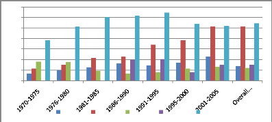
3.3.2 Claims o n private sector to GDP ratio

This indictor was suggested by some researchers as the best measurement of the level of financial depth as discussed in chapter two. The figure below indicates the level of financial depth in East African Countries had been this indicator used.

35

30

25

20

15

10

0

5

Rwanda Burundi Uganda Tanzania Kenya

Figure 2: Evolution i n average of claims o n private sector to GDP i n EAC

Kenya is still leading followed by Burundi whereas other countries are almost at the same level, which is very low below the average of 14.75%. Rwanda is the fourth with 7.05% while Uganda is the last in the group with 6.11%. Based on this indicator, we can say that Kenya enjoys a financial deepening four times that of Rwanda. However, Rwanda has been improving but at a slow rate compared to Burundi which made a significant improvement. This ratio for Burundi was more than three times that of Uganda and more than double that of Rwanda in recent period, while 30 years ago the difference between these countries was slightly small (less than 3%).

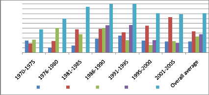
3.3.3 Domestic credit to GDP ratio

As the next figure shows, Burundi has been improving considerably from the last in row during the period 1970-1975 (with 9.45 %) to the 2^nd position (with 36.62%) for last two consecutive periods, from 1995 to 2005. Surprisingly, this indicator declined considerably in Rwanda's post genocide where it moved from 17.51% as the average for the war period of 1990-1995 to 11.54% for the last period 2001-2005 while the country was supposed to be putting enough effort in the credit to private sector to speed up the economic growth.

Financial Development and Economic Growth in Rwanda

45.00

40.00

50.00

35.00

30.00

25.00

20.00

15.00

10.00

0.00

5.00

Rwanda Burundi Uganda Tanzania Kenya

Figure 3: Evolution i n average ratio of domestic credit to GDP i n EAC

This ratio for Rwanda was below the EAC average throughout the period. Moreover, there is an increasing gap between Rwanda, the last in group, and Kenya, the first, from 11.46% over the period 1970-1975 to 27.97%. This is one among reasons that explain the gap in the level of economic development among these countries. Uganda and Tanzania too have the low ratio. Though several reasons can explain why Rwanda is lagging behind in financial development, civil war, insecurity and poor governance are paramount factors to the explanation. However, a detailed analysis is needed to explain why Tanzania and Uganda are not performing well in some areas while they enjoyed a relative stability, contrary to Burundi which was in war since 1993 up to 2005 and performed well.

3.4 Co nclusio

Rwandan economy has been growing during post genocide period but still the economy is at the lower level when compared to other countries. Indeed, the financial development is still low and below the average of the East African countries. When considering some indicators of the financial development over the period 1970-2005, Rwanda is almost the last within five countries though Uganda and Tanzania too are not performing well. This observation brings to mind the empirical question of the extent to which the level of financial development in Rwanda is linked with the level of economic growth. Therefore the following chapter presents the methodology followed to conduct this study.

Financial Development and Economic Growth in Rwanda

CHAPTER 4

METHODOLOGY

4.0 I ntroductio

This chapter presents the methods and techniques, the model, estimation techniques and types of data used in this study in investigating the causality among the proxies of financial development and economic growth.

4.1 Meaning and rationale of the model used

The use of VAR was motivated by its ability to capture the dynamic interaction of financial sector development and economic growth. A VAR is a direct generalization of the univariate AR(p) model to the case of a vector of variables and is used to express the dynamic correlations between the variables and hence is considered as an alternative to large-scale simultaneous equations structural models (Brooks, 2008).

It allows treating each variable as endogenous thus avoiding restrictions, judged incredible by Sims (1980), imposed by univariate AR, by specifying some variables as being exogenous. This model was chosen because the changes in indicators of financial development are possibly correlated with the disturbance term in the equation of economic growth. This is because an unobserved factor that influences growth of GDP may very well influence indicators of financial development, making them endogenous. Further more, this study joins other studies on the matter which used the VAR frame work, namely: Hassan and Jung-Suk (2007); Teame (2002); Sakutukwa (2008) and others.

4.2 Model specification and rationale of variables

In a VAR model, all variables have equations linking the change in that variable to its own current and past values and the current and past values of all the variables in the model, as it describes the dynamic evolution of a number of variables from their common history (Verbeek, 2004). The model is expressed

in a matrix form as:Yt = B + E^li^c__i AtYt_i + Et with:

V, = ( GRATE_S DEPTHBANKPRIVATESOPHT )

Yt : It is a 5×1 column vector of 5 variables including proxy measures of the financial development, B is a 5×1 column vector of constants, At and Y_t__i are

5×5 matrices of coefficients and lagged variables respectively, i is the lag length

to be determined by AIC criteria and et is a 5×1 column vector of error terms. Variables included in the models are:

GRATE = Growth rate of Real per capita GDP, following the works of Sinha and Macri (2001) and Kesseven et al (2007);

DEPTH = Claims on Private sector to GDP ratio considered as proxy of financial deepening, following the works of Karima and Holden (2001), Firdu and Struthers (2003) and Zhang et al (2007);

BANK = Domestic credit by deposit money bank and other banking institutions divided by total domestic credit;

PRIVATE = Claims on the non-financial private sector to gross domestic credit; SOPHT = Ratio of broad money to narrow money (M2/M1) as proxy of financial sophistication, following the work of Sakutukwa (2008).

BANK and PRIVATE are inspired by the work of Levine and King (1993). Unlike to them, we have included the domestic credit for other banking institutions in BANK to mitigate the drawbacks of this indicator as commercial banks are not the only financial institutions to provide valuable financial functions. However, there is still a weakness in these proxies in Rwanda because data used on assets of financial institutions do not include the UBPR which play an important role in Rwandan financial sector.

4.3. Model estimatio

4.3.1 Statio narity and coi ntegratio

Due to spurious regression resulting from nonstationary series in the regressions, we have conducted the tests for stationarity, using ADF to check whether the residual series are white noise. The tests for cointegration have been conducted to determine the form of the VAR to be estimated. In fact, trend stationary variables are estimated by OLS, if the variables contain stochastic trends and cointegrated, a VECM is used and finally if the variables are not stationary and not cointegrated, the model is estimated after the stochastic

trends have been removed by taking first differences of the data. All tests were run within Eviews 6.

4.3.2 Granger causality tests

To determine which sets of variables have a significant effects on each dependent variable, causality tests have been conducted by restricting the coefficient of the lags of a particular variable to zero (Wooldridge, 1990). The objective is to find out if changes in one variable do affect changes in another variable and vice versa. If this is the case, as explained by Brooks (2008), a sets of lags of the included variable should be significant and it would be said that there is a bi-directional causality, otherwise it should be said that some included variables are exogenous or no causality exists at all between variables had been all lags insignificant.

4.3.3. Variance decomposition and Impulse response

The ambiguity in interpreting individual coefficients in VAR model (Gujarati, 2004) motivated us to use the variance decomposition and impulse response function which trace out the response of the dependent variable in the VAR model to shocks in the error term for several periods in the future, keeping constant all other variables dated t and before.

4.4. The data source and measurement

The five considered time series are ratios we have computed from data provided by the IFS Yearbooks. The database includes 42 annual observations from 1964 to 2005. Unlikely to previous studies which used natural logarithm of the series, we did not find any graphical relationship, as advised by Gujarati (2004), which motivates a priori transformation of the data to log-log model.

4.5 Co nclusio

This chapter has presented the methodology that has been used in this study. The next chapter presents and analyses the results of econometric estimation. The main objective of the chapter is the hypothesis testing.

Financial Development and Economic Growth in Rwanda

CHAPTER 5

MODEL ESTIMATION AND FINDINGS

5.0 I ntroductio

So far we have presented the literature both on theoretical and empirical side on the causality between economic growth and financial development. It is now time to turn to the empirical testing of this relationship for Rwandan economy. This chapter presents the results obtained from econometric testing and discusses the meaning and reason behind the figures.

5.1 Test for statio narity

The footstep of this analysis is to determine whether the series are stationary or not. The ADF was used to test for stationarity of these series as it provides a superior test to DF, especially in case the residuals of the regression could be serially correlated. The lag length has been automatically selected by AIC from nine proposed lags and all three possibilities have been tested: neither intercept nor trend, intercept but no trend and both intercept and trend. In all cases, results were found similar irrespective of the model used.

Here we present the results from the general model including intercept with

trend, as depicted by: AYt₌f3_i + f3₂t + SYt_i + al _El:=i AYt__p + Et.

In addition, we have tested for the presence of trend in series, with the model:

Yt =cx +f3t + Et. The presence or the absence of the trend will be used for

subsequent tests. The table below presents the results: Table 2: ADF Test Statistics i n levels

Variable	t= statistics	Critical values at		Lag length		Decision at 5%
		5%				Presence of trend	GRATE
-3.59	-4.20	-3.52	1	Stationary		No	DEPTH
-6.11	-2.62	-1.94	0	Stationary		Yes

Variable	t= statistics	Critical values at		Lag length		Decision at 5%
		5%				Presence of trend	SOPHT
-3.36	-4.21	-3.52	2	Not stationary		Yes	BANK
-2.96	-4.19	-3.52	0	Not stationary		Yes	PRIVATE
-2.25	-4.21	-3.55	3	Stationary		Yes

The hypotheses tested are:

Ho: S = 0, the series are not stationary, ₎62 = 0, there is no trend

Ho: S * 0, the series are stationary, ₎62 * 0, there is a trend

After taking first differences of SOPHT and BANK, the series were found to be stationary at 1%, as the table below depicts:

Table 3: ADF Test Statistics with first difference

Variables	t=	Critical values at		Lag length		Decision
Statistic	1%	5%	selected			D(SOPHT)
-6.019	-4.205	-3.526	0	Stationary at 1%		D(BANK)
-6.759	-4.211	-3.529	1	Stationary at 1%

The above results conclude that GRATE, DEPTH and PRIVATE are I(0) while SOPHT and BANK are I(1). Therefore, VAR in levels cannot be applied.

5.2 Test for coi ntegratio

In econometric literature, it is not clear whether cointegration should be applied to only series integrated of the same order. Though Verbeck (2004) noted that the concept of cointegration can be applied to (nonstationary) integrated time series only and Dickey et al, quoted by Gujarati (2004), stipulated that Cointegration deals with the relationship among a group of variables, where (unconditionally) each has a unit root, however Brooks (2004) stressed that it is also possible to combine levels and first differenced terms in a VECM. The later therefore illustrates that cointegration can exist among variables not integrated of the same order.

Heij et al (2004) developed the mathematical proof of this view where they asserted that a cointegration relationship exists between stationary and nonstationary variables. If their mathematical proof is put in simple terms, there are three possibilities in VAR with many variables: If m: the number of variables, r= rank of the matrix of coefficients and also the number of cointegration relations, therefore:

· If all variables are stationary, r=m and all roots lie outside the unit cycle

· If all variables are not stationary, r=0, there are m unit roots or m stochastic trends.

· If some variables are stationary and others not stationary, r= 0<r<m, there are m-r unit roots, the polynomial have m-r common stochastic trends and there are r cointegrating relations.

As some variables are stationary and others not, Johansen cointegration test has been used to determine whether there exists a long-run relationship between these variables. This test was preferred to Engle-Granger approach because in case of five variables we may have more than one cointegrating relationship (Brooks, 2004).

a) Johansen coi ntegratio n test

Johansen trace test was used on the number of cointegrating relations with null hypothesis of no cointegration between series against the alternative hypothesis of existence of cointegration between the series. All variables enter the cointegration analysis in levels. This table depicts cointegrating vectors for each model with 4 lags.

Table 4: Number of coi ntegrati ng relations by model, at 5% level*

Data Trend:	None	None	Linear	Linear	Quadratic
Test Type	No Intercept	Intercept	Intercept	Intercept	Intercept
	No Trend	No Trend	No Trend	Trend	Trend
Trace	2	3	3	4	3
Max-Eig	0	1	3	4	3

*Critical values based on MacKinnon-Haug-Michelis (1999)

All five possibilities about the nature of deterministic trend assumption suggest
that the series are cointegrated. At least there is one cointegrating factor except
the Max-Eig method with neither intercept nor trend in data, which is unlikely to

be the case. The subsequent step is to determine whether an intercept or trend or both are included in the cointegrating relationship and to present the results of the selected model. The analysis of the nature of trend conducted showed that all variables except GRATE have significant intercept and trend. After estimating the selected model of both intercept and trend with 3 lags selected by AIC, the results were as follows:

Table 5: Unrestricted Coi ntegrati ng Rank Test (Trace)

Hypothesized No. of CE(s)	Eigenvalue	Trace Statistic	0.05 Critical Value	Prob.**
None *	0.890720	137.1029	88.80380	0.0000
At most 1	0.517635	55.19081	63.87610	0.2162
At most 2	0.306696	28.21578	42.91525	0.6091
At most 3	0.251814	14.66319	25.87211	0.6026
At most 4	0.100754	3.929364	12.51798	0.7523

Trace test indicates 1 cointegrating eqn(s) at the 0.05 level * denotes rejection of the hypothesis at the 0.05 level **MacKinnon-Haug-Michelis (1999) p-values

The statistic of 137.1 considerably exceeds the critical value (of 88.8) and so the null of no cointegrating vectors is rejected. But the 2^nd row shows that the null hypothesis of at most one cointegrating vector can not be rejected as trace statistic of 55.19 is less than critical value of 63.9. Therefore, there exists one cointegrating relation which means that the rank of the matrix (r) is one.

The results from trace test were the same if maximum eigenvalue test was considered. As there is one cointegrating vector, this allows us to estimate a VECM, in line with advice of Brooks (2004) of not using models in differences when cointegration is present, as this flows away important information and have no long-run solution.

5.3 Vector Error Correction Model (VECM)

The lag length was chosen based on AIC, which was consistent with LR and HQ. Noting that as data are annual observations, a maximum of 4 lags is reasonable, as suggested by Brooks (2004) based on the frequency of the observation and AIC picked 3 lags. The estimated output is presented in the appendix, but the table below presents the significant lags at 5% level.

Financial Development and Economic Growth in Rwanda

Table 6: Significant Vector Error Correction Estimates

Variable	Significant lags at 5% and their coefficients i n I l
D(GRATE)	CointEq1 [-2.03]	D(GRATE(-1)) [0.63]	D(GRATE(-2)) [0.25)	D(DEPTH(-1)) [0.69]
	D(DEPTH(-2)) [0.86]	D(DEPTH(-3)) [0.96]	D(Bank(-1)) [0.4]
D(DEPTH)	CointEq1 [-1.16]	D(DEPHT(-1)) [0.69]	D(DEPTH(-2)) [-0.79]	D(DEPTH(-3)) [-0.49]
	D(SOPHT(-1) [1.01]
D(SOPHT)	CointEq1 [-0.72]	D(PRIVATE(-2)) [-0.7]
D(BANK)	D(Bank(-1)) [-0.51]	D(PRIVATE(-1)) [1.11]	D(PRIVATE(-2)) [-1.26]	D(PRIVATE(-3)) [0.95]
D(PRIVATE)	D(PRIVATE(-1)) [0.62]	D(PRIVATE(-2)) [-0.52]	D(PRIVATE(-3)) [0.48]

The Error correction term showing the long-run equilibrium is estimated as:

CointEgl = GRATEt_i -- 0.057 SOPHTt_i + 0.0019 /31t -- 0.0019 /30

+ 0.332DEPHTt_1 -- 0.114 PRIVATEt_i + 0.298BANKt_1

In all equations, the cointegrating equation has a negative sign as expected and significant in three out of five equations. We note from the table above that in many equations of the VECM, the coefficients of lags of other variables are not significant, especially for PRIVATE which is determined solely by its own lags, SOPHT is explained by one lag from PRIVATE whereas for DEPTH only its own lags and 1 lag of SOPHT are significant.

The cointegration is strongly significant for GRATE, DEPTH and SOPHT. However, as noted by Brooks (2004), evaluation of the significance of variables in a VECM is based on the joint tests on all of the lags of a variable in the equation rather than individual coefficient estimates. Therefore we proceed to F test as indicated in the table below:

Table 7: F=statistics for VECM

Variables	D(GRATE)	D(DEPTH)	D(SOPHT)	D(Bank)	D(Private)
R^2	0.97	0.67	0.67	0.62	0.55
Adj R^2	0.95	0.41	0.41	0.33	0.19
F-stat	45.41	2.59	2.60	2.12	1.54

Critical values of F-statistic are taken from F-statistic table provided by Gujarati
(2004) and are 3.09; 2.2 and 1.84 for 1%; 5% and 10% respectively. The VECM

shows that for GRATE the null hypothesis being all coefficients are simultaneously zero is rejected at 1%, for DEPTH and SOPHT the null hypothesis is rejected at 5%, for BANK it is rejected at 10% and for PRIVATE the null hypothesis can not be definitely rejected.

The results suggest that there exist: a long-run relationship between growth rate of real per capita GDP and proxies of financial development, a long-run relationship between financial depth, rate of growth of real per capita GDP and other included measures of financial development and the same applies to financial sophistication. The F-test denies any long-run relationship between the ratio of credit to private sector to total domestic credit with GDP, and other measures of financial development and for the ratio of credit allocated by banks to total domestic credit when 5% level is considered.

5.4 The E ngle=Gra nger test

The test is meant to detect any short-term relationship between the variables and it is applied to test whether the changes in one variable can cause changes in another variable and vice-versa. As there is a long-run relationship between variables, the error correction term will be included in the Granger causality test for estimating a short-run relationship. It is worth noting that Granger causality test should be applied to stationary series (Sinha and Macri, 2001). Therefore, we have applied this test with differences in non-stationary series. When estimated the VAR model with differences in nonstationary variables to come up with lag length, the AIC and HQ criteria gave out 5 lags. The model to be estimated is:

M'at =0(0-Foci ~ 78 ~ ~~ ~ 98 ~

8 8 ~~ where Y_a and Yb are

~~~ ~~~

variables on which causality test is being applied. The hypotheses to be tested are:

H_o: âi=0, Yb does not Granger causes Ya

H1: âi ?0, Yb does Granger causes Ya

The results for Granger causality are presented in table below:

Financial Development and Economic Growth in Rwanda

Table 8: Marginal significance levels associated with joint F=test

Dependent variable	Lags of variables					Significant lags
	GRATE	DEPTH	DSOPHT	DBANK	PRIVATE
GRATE	0	9.8E-13	0.01503	0.60738	0.16923	DEPTH and SOPHT
DEPTH	0.99980	0	0.12400	0.99071	0.61635	None
DSOPT	0.00777	0.00338	0	0.54904	0.28578	GRATE and DEPTH
DBANK	0.99662	0.08847	0.73048	0	0.03597	PRIVATE
PRIVATE	0.25647	0.29164	0.38541	0.82127	0	None

The table above gives the probability values at 5% for the null hypothesis that all the lags of a given variable are jointly insignificant in a given equation. The second row after the headings shows that all the lags of DEPTH and DSOPHT are jointly significant in explaining the changes of GRATE (values less than 0.05). Indeed, both lags of GRATE and DEPTH jointly explain the changes in DSOPHT. Moreover, a part from the lags of PRIVATE which jointly explain DBANK, there is as well no causality between DEPTH and other variables as applied for PRIVATE.

The Engle-Granger causality suggests that in short-term, there is unidirectional causality from financial deepening to growth rate of real per capita GDP and bidirectional feedback between financial sophistication and growth rate of real per capita GDP. But other proxies of financial development do not seem to have affected economic growth, or being affected by economic growth.

5.5 Impulse responses and variance decompositions

The Granger Causality solves the problem of existence or not of variables with significant lags in the model but will not indicate whether there is a positive or a negative relationship between variables or how long the effects will take place. Fortunately, this information is given by Variance decomposition and Impulse responses.

5.5.1 Variance decompositio

Gebhard and Wolters (2007) define variance decompositions as a determinant
of how much the s-step-ahead forecast error variance of a given variable is

explained by innovations to each explanatory variable for s = 1, 2, etc. The estimated variance decompositions are as follows:

Table 9: Variance decomposition of GRATE

Period	S.E.	GRATE	DEPTH	SOPHT	BANK	PRIVATE
1	0.110866	100.0000	0.000000	0.000000	0.000000	0.000000
2	0.124707	82.69667	8.579287	3.272943	3.121836	2.329268
3	0.147683	68.46577	21.21998	2.911180	3.706309	3.696768
4	0.161082	63.06704	22.01977	5.362547	4.577584	4.973060
5	0.230705	30.74644	56.71985	2.944156	5.417225	4.172328
6	0.264102	25.86977	48.00195	11.86883	10.10530	4.154157
7	0.279128	27.88629	45.35033	11.21903	9.305821	6.238536
8	0.297045	24.98740	40.23873	20.10273	9.132219	5.538915
9	0.299774	25.47580	39.51314	20.12288	9.053579	5.834607
10	0.311132	25.82532	38.50044	21.06230	8.824819	5.787122

The data shows that in period 1, changes in Growth rate of GDP are due to its own shocks at 100%. However as time passes, the effects of shocks of other proxies of financial development to GDP increase significantly, especially financial depth shocks, which increase from 0 in period 1 to 56% in fifth period and represent more than 45% of all shocks on GDP from period 5-7 and nearly 40% above period 8. For Financial sophistication, although its shocks to GDP are low up to fifth period, they become important in the long-run, as they account from 10% - 20% of the whole shocks in GDP growth rate.

In long-run, BANK and PRIVATE exert some influence on Growth rate of GDP as they account for around 9% and 6 % respectively after the seventh period. This leads to a considerable decrease of responsiveness of growth rate of GDP to its own shocks from the range of 20% to 30 % after the fifth period.

Table 10: Variance decomposition of DEPTH

Period	S.E.	GRATE	DEPTH	SOPHT	BANK	PRIVATE
1	0.166228	6.593561	93.40644	0.000000	0.000000	0.000000
2	0.177693	5.794367	81.81403	10.71161	1.676598	0.003399
3	0.181328	6.251779	78.93336	11.59888	3.148914	0.067069
4	0.196067	5.909571	67.51985	21.31578	3.279901	1.974900
5	0.200638	5.771625	64.94746	20.47421	6.396104	2.410596
6	0.203363	5.642555	63.22212	20.70156	7.800917	2.632850
7	0.204559	5.698593	62.48965	20.49198	8.642176	2.677599

Financial Development and Economic Growth in Rwanda

Period S.E. GRATE DEPTH SOPHT BANK PRIVATE

8	0.206029	5.618773	61.74162	20.20135	9.476386	2.961867
9	0.206866	5.583026	61.38685	20.08648	9.998728	2.944921
10	0.209391	5.449760	61.67798	19.73869	10.25844	2.875138

From the first period, the shocks in GDP growth rate account for 6.59% of the shocks in DEPTH and no other variable exerts a shock on financial depth. However, as from the fourth period, the financial sophistication exerts a relatively higher significant influence on DEPTH than other variables, around 20%. Shocks in rate of GDP account still for around 5% and 2.8% for PRIVATE. It is noted that the impact of BANK shocks as well increase in the long-run, from 0% to 10.25% from the first period onwards.

Table 11: Variance decomposition of SOPHT

Period	S.E.	GRATE	DEPTH	SOPHT	BANK	PRIVATE
1	0.074312	26.69308	0.003523	73.30339	0.000000	0.000000
2	0.092146	18.38277	0.672448	74.86819	6.069340	0.007246
3	0.133858	9.698140	11.79599	67.75000	7.847544	2.908331
4	0.170257	6.012045	23.10979	54.15415	12.49342	4.230598
5	0.220413	3.774206	39.20184	37.55349	15.89273	3.577740
6	0.240093	3.239503	40.45313	31.95285	20.92763	3.426890
7	0.258410	2.844621	43.07799	28.56225	21.77780	3.737332
8	0.271110	2.841146	44.52708	26.18426	22.98927	3.458246
9	0.279182	2.780299	45.79558	24.69353	23.46618	3.264411
10	0.284385	2.707705	46.31954	23.86455	23.96186	3.146348

From the above table, the shocks in growth rate of GDP account for 26.69% in explaining changes in financial sophistication whereas its own shocks account for 73%, as other variables do not influence SOPHT in the first period. However, this order changes over time as financial depth takes over growth rate of GDP in explaining changes in financial sophistication. In fact, starting from the third period, shocks in financial depth lead to variability in financial sophistication by 11.7% compared to 9.6% of growth rate in GDP where still its own shocks account for more than 60%.

The influence of financial depth increases considerably up to 40% in sixth period and the own shocks decline to 31.95%, coupled with an increase in influence of BANK with 20.92% and a decrease in influence of GDP rate from 26.69% to 3.23% and remained at this level. The impact of PRIVATE shocks

remains low close to 3.5% whereas that of shocks from financial depth account for 40% to 45% in long-run, leaving the own shocks between 30% to 23% and BANK shocks around 23%.

Table 12: Variance decomposition of BANK

Period	S.E.	GRATE	DEPTH	SOPHT	BANK	PRIVATE
1	0.108855	0.758292	7.481317	2.693772	89.06662	0.000000
2	0.134533	2.800047	9.892457	3.375928	70.39165	13.53991
3	0.157558	3.654779	15.77366	3.449549	66.83704	10.28497
4	0.179687	4.319090	21.15028	5.165073	61.43189	7.933671
5	0.210744	5.307566	19.52585	10.44650	54.85325	9.866828
6	0.238217	5.969085	17.27681	17.65179	48.14008	10.96223
7	0.252272	6.237416	17.76269	20.31924	45.59069	10.08995
8	0.269294	6.611854	17.00039	23.16878	43.29296	9.926012
9	0.288331	6.654749	15.18331	25.94057	40.74650	11.47487
10	0.301548	6.780441	14.72203	27.67418	39.01775	11.80560

The part of changes to BANK due to its own shocks declines sharply from 89% in the first period to around 40% in long-run. In the short-run, shocks from DEPTH have a largest impact on BANK, varying from 7% to 21% whereas in long-run, shocks from SOPHT outweigh DEPTH shocks in explaining changes in BANK. Financial deepening and sophistication continue to exert a significant influence on the ratio of sources of credit (BANK), contributing to 40% of BANK shocks in the long-run (from the fifth period). Whereas, the shocks from growth rate of GDP and PRIVATE account for nearly 6% and 10% respectively.

Table 13: Variance decomposition of PRIVATE

Period	S.E.	GRATE	DEPTH	SOPHT	BANK	PRIVATE
1	0.058234	3.888004	8.796400	31.81067	0.011581	55.49335
2	0.113552	7.271370	4.966717	42.35623	0.397619	45.00806
3	0.147942	7.691150	8.030448	46.93222	1.178470	36.16772
4	0.185169	7.908759	8.726697	52.17925	0.932194	30.25310
5	0.228011	8.044798	8.260887	54.36709	0.645529	28.68169
6	0.267550	7.654312	6.582612	58.03725	0.605966	27.11986
7	0.295786	7.572517	6.240606	59.76170	0.888040	25.53714
8	0.325691	7.389561	5.409754	61.44629	0.957495	24.79690
9	0.352531	7.122818	4.661823	61.92543	1.102570	25.18736
10	0.376020	6.932724	4.193691	62.39958	1.343631	25.13037

Compared to other variables mentioned above, PRIVATE own shocks are
relatively small (55.5%) in the first period, and the shocks decline sharply to a

quarter in long-run. Shocks from Financial sophistication have a strong influence on PRIVATE and account for more than a half of total shocks from the fourth period onwards. Shocks from BANK are insignificants as they do not account for 2% and shocks from growth rate of GDP and DEPTH together account for nearly 10% of total PRIVATE shocks.

5.5.2 Impulse response models

Gebhard and Wolters (2007) define impulse responses as the measure of the effect of a unit shock of the variable i at time t on the variable j in later periods. So for each variable from each equation separately, a unit shock is applied to the error term and the effects upon the VAR system over time are noted. Details of impulse responses are presented in appendices and their summarized results are:

o Positive shocks of DEPTH and BANK to GDP growth rate but negative shocks from SOPHT and PRIVATE.

o Positive shocks on DEPTH from GDP growth rate, financial sophistication and BANK in short-run. Moreover, SOPHT and BANK have positive shocks on DEPTH in long-run and negative PRIVATE shocks on DEPTH.

o Positive shocks on financial sophistication from BANK and growth rate of GDP in short-run and negative shocks from growth rate of GDP, DEPTH and PRIVATE in long-run.

o Positive shocks on BANK from PRIVATE and negative shocks from growth rate of GDP and financial sophistication.

o Negative shocks on PRIVATE from all variables.

In the results above, the ordering was GRATE, DEPTH, SOPHT, BANK, and PRIVATE. Unfortunately, the main drawback of Variance decomposition and Impulse responses is that if the variable order is altered the results will change too. For independent results from variable order, a priori knowledge about the order is required, but not easy in most interdependent financial time series data.

5.6 Discussion of findings

The tests revealed a long-run relationship between the Growth rate of real per
capita GDP and 4 proxies of financial development. Precisely, financial

deepening and financial sophistication were revealed to be associated to this rate of GDP in the long-run. This implies that as the economy allocates more credit to the private sector, as new financial instruments are introduced in Rwandan financial system, with time, then the level of economic growth will be affected. The causality test, Variance decomposition and impulse responses show that financial deepening influences positively economic growth. But no bidirectional causality detected from growth rate of GDP to financial deepening.

These results confirm the importance of the level of financial depth for Rwandan economic growth, unlikely to the conclusion of some researchers who used panel data analysis and affirmed the irrelevance of the level of financial deepening on economic growth for Sub-Saharan Africa and poor countries in general, as noted by Hassan and Jung-Suk (2007) and Michael and Giovanni (2001). Our results do agree with the conclusions of Zhang et al (2007) in China, Demetriades and Luintel (1996) in India and Sakutukwa (2008) in Zimbabwe.

The causality test and variance decomposition showed a bi-directional influence between the level of financial sophistication and economic growth. Surprisingly, impulse responses show that this relationship is negative and a mere interpretation may conclude that financial sophistication aggravates economic growth. But there can be an intuitive explanation of this situation: «the true measurement of the financial sophistication in Rwanda». The used growth rate of real per capita GDP excludes effects of inflation and the increase in the ratio of M2 to M1 used as proxy of financial sophistication could imply increase in money supply due to inflationary pressure rather than financial innovation.

This is the case for Rwanda where post genocide economy was characterized by high rate of inflation and volatility in exchange rate. Despite the increase in the quasi-money which resulted in the increase of the ratio of M2 to M1, there was no E-banking in Rwanda up to 2005, no remarkable new financial instruments and ATM cards were recent in few banks, in major towns only.

No link was found between economic growth and allocation of credit. Were the
relationships to be established by Granger causality, the impulse responses

show that the relationship would be negative. The absence or a negative relationship between the growth rate of real per capita GDP and PRIVATE, and between PRIVATE and DEPTH can be explained by the allocation of credit. Credit devoted to agricultural sector which employs more than 80% of the population was less than 1.5% of total credit to private sector while the manufacturing, trade, restaurants and hotels received more than 60% of the total credit, while these sectors employ less than 5% of the population and contributed to only 17.4% in GDP in 2005.

Moreover, some loans were given to no profitable projects and non credit worthy customers as indicated by the high level of defaulters which led to bank crisis in former BACAR, BICDI and many MFIs. These findings of negative relationship between credit allocation and economic growth conquer with findings of Karima and Holden (2001), in a panel of 30 developing countries.

5.7 Co nclusio

The study finds a strong positive causality from financial deepening to economic growth and a negative bi-directional feedback between economic growth and financial sophistication, in the short-run, and a long-run relationship between economic growth and proxies of financial development.

The lack of short-run relationship between economic growth and the credit allocation, from the source (commercial bank versus central bank) to the users (private sector versus public sector) has been confirmed, while in the long-run, variance decompositions and impulse responses showed a minor relationship between economic growth rate and credit allocation. The found negative link between level of economic growth and financial sophistication is explained by the lack of accuracy of measurement of financial sophistication in Rwanda. The next chapter will therefore put forward the general conclusions and recommendations of the study.

Financial Development and Economic Growth in Rwanda

CHAPTER 6

CONCLUSIONS AND RECOMMENDATIONS

6.0 I ntroductio

This study intended to examine the bi-directional influence between financial development and economic growth in Rwanda from 1964 to 2005. Chapter one presented the existing problem which was the rationale of our study alongside the objectives, research hypotheses among others. Chapter two reviewed the literature on the subject both on theoretical and empirical ground. In chapter three, a comparative analysis of the level of financial development within East African countries has been carried out and revealed a weak level of financial development in Rwanda. The results indicate that Rwanda either takes the fourth or the last position among five countries.

In chapter four, we have explained the methodology followed, focused on a VAR with five variables, namely: the indicator of financial deepening, financial sophistication and other two indicators of the credit allocation, and the growth rate of real per capita GDP was used as proxy of economic growth. The fifth chapter has been devoted to econometric testing. This chapter summarizes the results of the study and gives recommendations as well as areas for further studies.

6.1 Summary of findings

The empirical results demonstrated both a short and a long-run relationship between both financial depth and sophistication and economic growth. For financial deepening, the causality runs from financial deepening to economic growth and for financial sophistication, the causality is bi-directional but negative. As some studies have concluded, we have not found any evidence of the link between credit allocation and economic growth and even if the relationship was to be significant, it would be negative. This is explained by the pattern of the credit to private sector which has become increasingly skewed to service sector with less employment and loan defaulters rather than to agriculture and businesses for productive investments.

All in all, we found that the level of financial development matters most for Rwandan economy, contrary to the irrelevance of the financial development on economic growth in cross-sectional analysis for developing countries confirmed by previous studies. The reason being that their analysis does not take into consideration country's unique characteristics or the results are biased by the presence of outliers in their regression, due to size inequalities of countries within a region.

The first and fourth hypotheses were partly confirmed while the second and third could not be confirmed. The study has attained its objectives and recommendations for further strengthening both Rwandan financial sector and Rwandan economy in general have been suggested.

6.2 Policy recommendations

Based on the results of the study, it is urgent that Rwandan government takes the financial sector as a pillar of economic growth which can replace non performing industrial sector and agriculture. The emphasis put on it can allow Rwanda to be the net exporter of financial services within East African Community and Commonwealth where Rwanda was admitted recently, as we do not have any comparative advantage in remaining sectors.

The emphasis should be put on the level of financial intermediation through increase in the credit allocated to private sector. It is however important to note that the allocation of the credit should be changed from private consumption and services to agriculture and other investment projects like construction sector. Additionally, credit allocation should be based on the profitability of the investment rather than personal considerations or values.

More so, Rwandan government should accelerate financial innovations which are currently very low, by making compulsory: distribution of ATM cards by banks upon bank account opening; and the use of credit cards as a means of payment in strong legalized supermarkets and shops, as a first step in the introduction of card-based system of payment.

BPR S.A has provided evidence that bank branch proximity is a key factor in bank profitability. It is therefore, recommended that other commercial banks in Rwanda should open at least one branch in each district. Due to the absence of positive impact of financial innovations on economic growth explained by inflationary pressures and exchange rate depreciation, the Government of Rwanda should put more efforts on price and exchange rate stability.

The introduction of OTC market was a good step for financial development. However, a lot need to be done regarding empowering the saving capacity of Rwandans, by policy measures enhancing an equal distribution of income, poverty eradication and the fight against rampant unemployment. We believe these factors to have been the reasons for the absence of transactions on OTC market rather than lack of public awareness as reported by newspapers.

For employed population, the government of Rwanda should ensure that the salary is enough to cover the subsistence needs so that saving is possible. This can be done through the minimum wage legislation since a larger group of employed people earn even what is not enough for family expenses. In such conditions, any policy aimed at saving mobilization would futile.

We can not claim that the study has explored all areas of the problem. For instance, we have not used the level of stock market development in our econometric analysis due to lack of data as the existing OTC started in 2008.

6.3 Areas for further research

Studies need to be conducted to determine best proxies of financial development in Rwanda, especially for financial innovations, as the used ratio of M2 to M1 may reflect the increase in classical saving functions rather than diversification of financial instruments and use of modern technology in the financial sector. Indeed, a cross-sectional study in EAC would be interesting, to assess how developed financial systems are and how they are relevant to economic growth.

Financial Development and Economic Growth in Rwanda

REFERENCES

1. Abebe, A. (1990), «Financial Repression and its Impact on Financial development and Economic Growth in the African Least Developed Countries", Savings and Development, no1, X1V, pp. 23-55.

2. Alison, T., Geda, A., Le Billon, P., Murshed, S.M. (2001), «Financial Reconstruction in Conflict and 'Post-Conflict' Economies", Paper presented at the Conference of the Finance and Development Research Programme, pp. 5-6.

3. Beck, T., Demirguc-Kunt, A. and Maksimovic, V. (2006), «Financing Patterns around the World: Are Small Firms Different?", World Bank mimeo.

4. Bodie. Z, Kane A. and Marcus A. (2008), Essentials of Investments, McGraw -Hill International ed, 7ed, New York, USA

5. Brooks, C.(2008), "Introductory Econometrics for Finance", 2nd ed, The ICMA Centre, University ^of Reading, Cambridge University Press

6. Buffie, E. F. (1984), «Financial Repression: The New Structuralist and Stabilization, Policy in Semi-industrialized economies", Journal of Economic Development, 14,3, pp. 303-322.

7. Cameron, R. (1961), «France and Economic Development in Europe", Princeton University Press, Princeton, NJ.

8. CIA World Factbooks, 2003-2008, www.cia.gov

9. CMAC, www, cmac.gov.rw

10. Demetriades, P.O and Luintel, K.B (1996), «Financial Development, Economic Growth and Banking Sector Controls: Evidence from India", The Economic Journal, The Journal of the Royal Economic Society, pp. 359- 374.

11. Demirgüç-Kunt, A. and Maksimovic, V. (1998), «Law, Finance, and Firm Growth", Journal of Finance 53, pp. 2107-2137.

12. Diaz-Alejandro, C.(1985), «Good-bye Financial Repression, Hello Financial Crisis", Journal of Development Economics, 19 (1/2), 1-24.

13. Douglas, K. (2003), «The Finance Growth Nexus: Evidence from Sub-Saharan Africa", IAER: May 2003, Vol. 9, no. 2.

14. Dushimumukiza, D. (2006), «Correlation entre le Taux de Change et la Balance des Paiements», UNR, Huye-Rwanda, Unpublished Dissertation.

15.

Firdu, G. and Struthers, J. (2003), «The McKinnon-Shaw Hypothesis: Thirty Years on: A Review of Recent Developments in Financial Liberalization Theory", Paper presented at DSA Annual Conference on «Globalisation and Development», Glasgow, Scotland, September 2003.

16. Friedman, M. and Schwartz, A.J. (1963), «A Monetary History of United States, Princeton», Princeton University press

17. Fry, M.J. (1989), «Financial development: Theories and recent experience", Oxford Review of Economic policy, vol 5 no 4

18. Fry, M.J. (1997), «In Favour of Financial liberalization", The Economic Journal, Vol. 107, No. 442, pp.754-770.

19. Gebhard, K. and Wolters, J.(2007), «Introduction to Modern Time series", Springer-Verlag Berlin Heidelberg.

20. Greenwood, J. and Jovanovic, B. (1990), «Financial Development and the Development of Income"; Journal of political economy, Vol. 98

21. Gujarati, D. (2004), «Basic Econometrics", 4^th edition, The MacGraw-Hill companies.

22. Habyalimana, S. (2007), «Access to Finance Through Value 0hains: Lessons From Rwanda", AEGIS European Conference on African Studies 11-14 July 2007, Leiden, the Netherlands.

23. Hassan, M. K. and Jung-Suk Y. (2007), «Financial Development and Economic Growth: New Evidence from Panel Data", Journal of Economic Literature, G21.

24. Heij, C, Paul, B, Philip, H.F, Kloek, T and Herman, K.V. (2004), «Econometric Methods with application in Business and Economics", Oxford University Press Inc., New York.

25. IFAD, www.ifad.org

26. IMF (1994 and 2005), «International Financial Statistics Yearbooks", Vol XLVII and Vol LVIII, Washington, D.0

27. IMF(2009), «World Economic Outlook Database", April 2009 and October 2009

28. Jankee, K. (2006), «Banking Controls, Financial deepening and Economic Growth in Mauritius", African Review of Money, Finance and Banking, pp. 77-98.

29. Kantengwa. A, (2009), «Financial Cooperatives in Rwanda: Historical Background and Regulation", Kigali, Rwanda.

30. Karima, S. and Holden, K. (2001), «Does Financial Development affect Growth?", Liverpool John Moores University, UK

31. Kesseven, P., Boopen, S. and Ramesh, D. (2007), «Financial Development and Economic Growth in Africa: a Dynamic Panel Data Analysis", International Journal of Business Research.

32. Koðar, C.I (1995), «Financial Innovations and Monetary Control", The Central Bank Of The Republic Of Turkey, Research Department, Discussion Paper No: 9515

33. Kuznets, S. (1955), «Economic Growth and Income Inequalities", An American economic review, Vol. 45

34. Levine, R. (1997), «Financial development and economic growth: Views and Agenda», Journal of economic Literature XXXV, pp. 688-726.

35. Levine, R. (2001), « Stock Market, Growth and Tax Policy", Journal of finance, Vol. 46, no.4

36. Levine, R. and King, R.G. (1993), "Financial Entrepreneurship and Growth. Theory and Evidence", Journal of Monetary Economic.

37. Levine, R. and Zervos, S. (1996), "Stock markets, Banks and Economic Growth", World Bank Policy Research Working Paper, No 1690

38. Liu, L., Yunhua, B. Fleisher, Hongyi Li, (1994), «Financial Intermediation, Inflation and Capital Formation in Rural China", China Economic Review.

39. Loayza N., K. Schmidt-Hebbel, and L. Serven (2000), «What Drives Private Saving Across the World?», Review of Economics and Statistics, May 2000, 82(2), pp. 165-181.

40. Lucas, R. E. (1988), «On the Mechanics of Economic Development", Journal of monetary economics.

41. Margaret z. C. (2004), «Geographic Deregulation of Banking and Economic Growth", Journal of Money, Credit and Banking, Vol. 36, No. 5 (Oct., 2004), pp. 929-942.

42. Mauro, P. (1995), «Corruption and Growth", Quarterly Journal of economics.

43. McKinnon, R.I (1973), «Money and capital in Economic Development", Washington, D.C, Brookings institutions.

44.

Michael, W. K. and Giovanni, P. O. (2001), «Capital Account Liberalization, Financial depth, and Economic Growth", Federal Reserve Bank of Boston, Boston.

45. Murgatroyd. P, Dry. J, Power T. and Postgate W. (2007), «Rwanda financial sector development program, First initiative», Kigali, Rwanda

46. National Bank of Rwanda (2004, 2008 and 2009), «Annual report 2003, 2007 and 2008", Kigali, Rwanda

47. National Institute of Statistics of Rwanda (2008, 2007), «Rwanda Development Indicators- 2006, 2007", Rwanda.

48. Rajan, R.C and Zingales, ^L. (1998), «Financial Dependence and Growth", American Economic Review 88, pp. 559-586.

49. Raymond, F. and Love, I. (2004), «Financial development and Growth in the Short and Long Run", World Bank, Policy Research Paper 3319

50. Robinson, J. (1952), «The Generalization of the General Theory , The Rate of Interest and Other Essays", London, Macmillan, pp. 69 -142

51. Sakutukwa, T. (2008), «The Financial Sector Deepening, Sophistication and Growth Nexus", University of Zimbabwe, Unpublished MA thesis.

52. Schumpeter, J.A. (1911), "The Theory of Economic Development, An Inquiry into the Profits, Capital, Credit Interests and the Business Cycles", Cambridge, MA: Harvard, University press.

53. Shaw, E. S. (1973), "Financial deepening in Economic Development", New York, Oxford University Press.

54. Sims, C. A (1980), «Macro economics and Reality", Econometrica

55. Singh, A. (1997), «Financial Liberalization, Stock Market and Economic Development,» The Economics Journal, 107, 771-782

56. Sinha, D. and Macri, J. (2001), «Financial Development and Economic Growth: The Case of eight Asian countries», Journal of Economic Literature, C32, E51, 010

57. Spears, A. (1991), «Financial Development and Economic Growth-Causality tests", Atlantic Economic Journal.

58. Stiglitz, J. E. (I 994), «The Role of the State in Financial Markets", In Proceedings of the World Bank Annual Bank Conference on Development Economics 1993 (ed. M. Bruno and B. Pleskovic), Washington, D.C: World Bank, pp. I9-52.

59.

Stiglitz, J.E and Andrew, W. (1981), «Credit Rationing in Market with Imperfect Information», American Economic Review, 71 (3), pp. 393-410.

60. Teame, G. (2002), «Financial Development and Economic Growth in Sub-Saharan African Countries: Evidence from Time Series analysis», Morehead State University, Morehead, KY 40351, USA.

61. Thangavelu, S.M. (2004), «Financial Development and Economic Growth in Australia: An Empirical analysis", Empirical economics, vol 29, issue 2, pp. 247-260

62. Tufano, P. (2002), «Financial innovations", The Handbook of the Economics of Finance, North Hollande.

63. UNDP (2004), «Human Development Report 2003", New York

64. United Nations Population Division (2008), «World Population Prospects", Revision, www.un.org/esa/population/

65. United Nations Statistics Division, http://unstats.un.org/unsd/demographic/

66. Verbeek, M. (2004), A guide to modern econometrics, 2^nd ed, John Wiley & Sons, England.

67. Wooldridge, J. M, (1990), «Introductory econometrics", a modern approach, 2^nd ed,

68. World Bank, «World Development indicators Database",
http://web.worldbank.org.

69. Yongfu, H. (2005), «What determines financial development?", Discussion Paper No. 05/580, University of Bristol.

70. Zhang. J, Guanghua W. and Yu J. (2007), «The Financial Deepening: Productivity Nexus in China: 1987-2001», World Institute for Economic development research, the United Nations University, Research Paper No. 2007/08.

Financial Development and Economic Growth in Rwanda

APPENDICES

Appendix A: Comparison of financial development i n EAC Table A.1: Average ratio of liquid liabilities to GDP i n EAC

Period	Rwanda	Burundi	Uganda	Tanzania	Kenya
1970-1975	14.07	11.24	21.08		31.05
1976-1980	13.94	14.13	17.48		38.04
1981-1985	12.79	17.69	11.43		38.97
1986-1990	16.03	17.57	11.11	18.59	42.69
1991-1995	16.49	19.31	10.75	23.41	50.05
1995-2000	15.63	19.82	14.72	20.00	39.45
2001-2005	18.77	25.80	19.67	23.48	39.87
Overall average	15.35	17.75417	15.345	21.68	39.77
Rank	4	3	5	2	1

The regional average is 21.98

For Tanzania, data are available as from 1988.

Source: Author's calculation from data provided by World Development Indicators database

Table A.2: Average ratio of claims o n private sector to GDP i n EAC

Period	Rwanda	Burundi	Uganda	Tanzania	Kenya
1970=1975	3.39	5.82	8.98		19.11
1976=1980	5.00	7.46	8.93		25.66
1981=1985	6.45	10.65	4.65		30.16
1986=1990	8.19	11.21	3.24	9.85	30.82
1991=1995	7.08	16.98	4.06	10.19	32.32
1995=2000	8.60	19.28	5.72	4.05	26.97
2001=2005	11.41	25.73	6.62	7.52	25.83
Overall average	7.06	25.73	6.11	7.68	27.18

The regional average is 14.75

For Tanzania, data are available as from 1988.

Source: Author's calculation from data provided by World Development Indicators database

Financial Development and Economic Growth in Rwanda

Table A.3: Average domestic credit to GDP ratio i n EAC

Period	Rwanda	Burundi	Uganda	Tanzania	Kenya
1970-1975	12.39	9.45	13.32		23.85
1976-1980	5.27	12.09	25.36		34.98
1981-1985	7.39	23.96	19.06		47.01
1986-1990	14.15	24.61	25.10	28.21	49.64
1991-1995	17.51	20.89	12.69	28.38	50.91
1995-2000	12.36	27.52	8.01	13.07	40.38
2001-2005	11.54	36.62	11.81	10.11	39.51
Overall average	11.54	21.81	16.48	19.02	40.42

Source: Author's calculation from data provided by World Development Indicators database

Appendix B: Granger causality test

Pairwise Granger Causality Tests Date: 12/15/09 Time: 21:35 Sample: 1964 2005

Lags: 5

Null Hypothesis:	Obs	F-Statistic	Probability
DEPTH does not Granger Cause GRATE	36	55.5580	9.8E-13
GRATE does not Granger Cause DEPTH		0.02080	0.99980
DSOPHT does not Granger Cause GRATE	36	3.52734	0.01503
GRATE does not Granger Cause DSOPHT		4.06239	0.00777
DBANK does not Granger Cause GRATE	36	0.73037	0.60738
GRATE does not Granger Cause DBANK		0.06634	0.99662
PRIVATE does not Granger Cause GRATE	36	1.70944	0.16923
GRATE does not Granger Cause PRIVATE		1.40536	0.25647
DSOPHT does not Granger Cause DEPTH	36	1.93549	0.12400
DEPTH does not Granger Cause DSOPHT		4.77110	0.00338
DBANK does not Granger Cause DEPTH	36	0.10249	0.99071
DEPTH does not Granger Cause DBANK		2.18163	0.08847
PRIVATE does not Granger Cause DEPTH	37	0.71712	0.61635
DEPTH does not Granger Cause PRIVATE		1.30701	0.29164
DBANK does not Granger Cause DSOPHT	36	0.81696	0.54904
DSOPHT does not Granger Cause DBANK		0.55867	0.73048
PRIVATE does not Granger Cause DSOPHT	36	1.32527	0.28578
DSOPHT does not Granger Cause PRIVATE		1.09960	0.38541
PRIVATE does not Granger Cause DBANK	36	2.85052	0.03597
DBANK does not Granger Cause PRIVATE		0.43293	0.82127

Financial Development and Economic Growth in Rwanda

Appendix C: Vector Error Correction Estimates, model 4 i n Eviews

Vector Error Correction Estimates

Date: 12/15/09 Time: 20:04

Sample (adjusted): 1969 2005

Included observations: 37 after adjustments Standard errors in ( ) & t-statistics in [ ]

Cointegrating Eq:	CointEq1
GRATE(-1)	1.000000
DEPTH(-1)	0.332100
	(0.11144)
	[ 2.98006]
SOPHT(-1)	-0.057857
	(0.05848)
	[-0.98942]
BANK(-1)	0.298156
	(0.08532)
	[ 3.49472]
PRIVATE(-1)	-0.114378
	(0.06522)
	[-1.75373]
@TREND(64)	0.001995
	(0.00120)
	[ 1.66116]
C	-0.109284
Error Correction:	D(GRATE)	D(DEPTH)	D(SOPHT)	D(BANK)	D(PRIVATE)
CointEq1	-2.032065	-1.163989	-0.720578	-0.251856	-0.157054
	(0.22472)	(0.56523)	(0.28767)	(0.39386)	(0.22592)
	[-9.04258]	[-2.05932]	[-2.50489]	[-0.63946]	[-0.69519]
D(GRATE(-1))	0.635997	0.512173	0.247474	-0.009307	0.047996
	(0.18428)	(0.46352)	(0.23590)	(0.32299)	(0.18527)
	[ 3.45116]	[ 1.10496]	[ 1.04904]	[-0.02882]	[ 0.25906]
D(GRATE(-2))	0.251038	0.263218	0.130006	0.132536	0.092150
	(0.10913)	(0.27450)	(0.13970)	(0.19127)	(0.10971)
	[ 2.30028]	[ 0.95890]	[ 0.93058]	[ 0.69292]	[ 0.83991]
D(GRATE(-3))	0.087797	-0.105592	-0.016569	-0.043783	-0.023816
	(0.07554)	(0.19001)	(0.09670)	(0.13240)	(0.07594)
	[ 1.16222]	[-0.55573]	[-0.17134]	[-0.33069]	[-0.31360]
D(DEPTH(-1))	0.695429	-0.758239	0.215837	0.068061	0.104795
	(0.08377)	(0.21071)	(0.10724)	(0.14683)	(0.08422)

Financial Development and Economic Growth in Rwanda

[ 8.30121] [-3.59845] [ 2.01265] [ 0.46355] [ 1.24430]

D(DEPTH(-2)) 0.866526 -0.790565 -0.013760 -0.157924 -0.021024

(0.09146) (0.23004) (0.11708) (0.16029) (0.09194)

[ 9.47464] [-3.43667] [-0.11753] [-0.98523] [-0.22866]

D(DEPTH(-3)) 0.963663 -0.491379 0.112484 0.041585 0.061428

(0.08089) (0.20346) (0.10355) (0.14177) (0.08132)

[ 11.9130] [-2.41509] [ 1.08628] [ 0.29332] [ 0.75537]

D(SOPHT(-1)) -0.090012 1.010779 0.171212 0.449488 -0.118463

(0.17793) (0.44754) (0.22777) (0.31185) (0.17888)

[-0.50588] [ 2.25852] [ 0.75168] [ 1.44136] [-0.66225]

D(SOPHT(-2)) 0.431769 0.540692 0.505270 0.034316 -0.012187

(0.23061) (0.58004) (0.29520) (0.40417) (0.23184)

[ 1.87230] [ 0.93217] [ 1.71159] [ 0.08490] [-0.05257]

D(SOPHT(-3)) 0.437132 1.215253 0.181885 -0.170377 -0.015982

(0.24017) (0.60408) (0.30744) (0.42093) (0.24145)

[ 1.82010] [ 2.01173] [ 0.59161] [-0.40476] [-0.06619]

D(BANK(-1)) 0.408020 -0.117947 0.304158 -0.517110 -0.034987

(0.12039) (0.30282) (0.15412) (0.21101) (0.12103)

[ 3.38905] [-0.38950] [ 1.97355] [-2.45067] [-0.28907]

D(BANK(-2)) 0.188578 -0.139547 0.219934 -0.160104 0.000816

(0.13695) (0.34446) (0.17531) (0.24002) (0.13768)

[ 1.37701] [-0.40512] [ 1.25456] [-0.66704] [ 0.00593]

D(BANK(-3)) 0.071952 0.000327 0.039480 -0.148662 0.020364

(0.11299) (0.28420) (0.14464) (0.19803) (0.11359)

[ 0.63680] [ 0.00115] [ 0.27296] [-0.75071] [ 0.17927]

D(PRIVATE(-1)) -0.165391 0.078972 0.292223 1.119834 0.627575

(0.22021) (0.55388) (0.28189) (0.38595) (0.22138)

[-0.75106] [ 0.14258] [ 1.03664] [ 2.90150] [ 2.83481]

D(PRIVATE(-2)) 0.118144 0.578400 -0.701639 -1.260416 -0.528714

(0.26649) (0.67028) (0.34113) (0.46706) (0.26790)

[ 0.44334] [ 0.86293] [-2.05680] [-2.69864] [-1.97352]

D(PRIVATE(-3)) -0.370708 -0.594595 0.504420 0.953775 0.488117

(0.23649) (0.59482) (0.30273) (0.41448) (0.23775)

[-1.56756] [-0.99962] [ 1.66624] [ 2.30115] [ 2.05311]

C -0.037309 -0.056214 -0.008053 0.001519 0.010289

(0.01270) (0.03194) (0.01625) (0.02225) (0.01277)

[-2.93824] [-1.76007] [-0.49541] [ 0.06827] [ 0.80600]

R-squared 0.973212 0.675205 0.675713 0.629321 0.553143

Adj. R-squared 0.951782 0.415368 0.416283 0.332778 0.195658

Sum sq. resids 0.075749 0.479224 0.124129 0.232683 0.076558

S.E. equation 0.061542 0.154794 0.078781 0.107862 0.061870

F-statistic 45.41337 2.598578 2.604607 2.122192 1.547317

Financial Development and Economic Growth in Rwanda

Log likelihood 62.03727	27.90961	52.90027	41.27567	61.84092
Akaike AIC -2.434447	-0.589708	-1.940555	-1.312199	-2.423834
Schwarz SC -1.694296	0.150443	-1.200404	-0.572047	-1.683682
Mean dependent -0.010551	0.003519	0.021542	0.013534	0.015225
S.D. dependent 0.280267	0.202448	0.103115	0.132048	0.068986
Determinant resid covariance (dof adj.)	7.67E-12
Determinant resid covariance	3.54E-13
Log likelihood	267.8841
Akaike information criterion	-9.561301
Schwarz criterion	-5.599313

Appendix D: Impulse responses Table D.1: Response of GRATE

Period	GRATE	DEPTH	SOPHT	BANK	PRIVATE
1	0.110866	0.000000	0.000000	0.000000	0.000000
2	0.023867	0.036527	-0.022561	0.022034	-0.019033
3	0.045515	0.057392	-0.011222	0.017968	-0.021072
4	0.037837	0.032946	-0.027505	0.019478	-0.022002
5	-0.000736	-0.156447	-0.013251	0.041177	-0.030501
6	0.040981	0.057379	-0.081924	0.064538	-0.026016
7	0.060685	0.043036	0.021506	0.014210	-0.044306
8	0.017915	0.013092	-0.094851	0.028416	-0.005168
9	0.029084	-0.001842	-0.018589	0.008837	-0.018867
10	0.045891	0.041967	-0.048016	0.020167	-0.018944

Table D.2: Response of DEPTH

Period	GRATE	DEPTH	SOPHT	BANK	PRIVATE
1	0.042684	0.160654	0.000000	0.000000	0.000000
2	0.002765	0.004773	0.058156	-0.023008	0.001036
3	-0.015034	-0.010982	-0.020773	0.022494	0.004580
4	0.014703	0.001705	0.066186	0.015017	-0.027150
5	0.007187	0.013749	0.006914	0.036248	-0.014533
6	-0.003185	0.001136	0.017871	0.025522	-0.010883
7	-0.007141	0.001467	-0.003656	0.019751	-0.005619
8	-0.000708	0.007714	0.000523	0.020156	-0.011697
9	-0.002032	0.007852	-0.004548	0.016009	-0.001729
10	0.000490	0.027798	-0.007655	0.014797	-0.000593

Financial Development and Economic Growth in Rwanda

Table D.3: Response of SOPHT

Period	GRATE	DEPTH	SOPHT	BANK	PRIVATE
1	0.038394	-0.000441	0.063624	0.000000	0.000000
2	0.009317	-0.007543	0.048052	0.022701	-0.000784
3	0.013298	-0.045349	0.076042	0.029846	-0.022814
4	0.002239	-0.067715	0.059652	0.047068	-0.026556
5	-0.009531	-0.111113	0.050461	0.064027	-0.022623
6	-0.005816	-0.065377	0.013228	0.065899	-0.015404
7	-0.005667	-0.073800	0.025564	0.049785	-0.022808
8	-0.013739	-0.062946	-0.013155	0.048529	-0.006798
9	-0.008875	-0.054465	0.001052	0.037321	-0.001589
10	-0.004777	-0.042031	-0.007326	0.033000	-0.000490

Table D.4: Response of BANK

Period	GRATE	DEPTH	SOPHT	BANK	PRIVATE
1	-0.009479	-0.029774	-0.017866	0.102732	0.000000
2	-0.020419	-0.030066	-0.017083	0.046759	0.049504
3	-0.020012	-0.046101	-0.015663	0.062062	-0.010128
4	-0.022073	-0.053973	-0.028484	0.056945	0.002892
5	-0.031028	-0.042932	-0.054515	0.067285	0.042668
6	-0.032095	-0.033648	-0.073330	0.054373	0.042879
7	-0.024130	-0.038732	-0.053985	0.041184	0.014162
8	-0.028729	-0.032004	-0.062213	0.048800	0.027874
9	-0.027158	-0.017147	-0.069020	0.049787	0.048387
10	-0.025162	-0.027646	-0.059990	0.040059	0.034574

Table E.5: Response of PRIVATE

Period	GRATE	DEPTH	SOPHT	BANK	PRIVATE
1	-0.011483	-0.017272	-0.032845	-0.000627	0.043381
2	-0.028385	-0.018496	-0.066202	-0.007133	0.062621
3	-0.027309	-0.033425	-0.069358	-0.014376	0.045964
4	-0.032068	-0.035136	-0.087287	-0.007855	0.049569
5	-0.038349	-0.036091	-0.101852	-0.003997	0.067366
6	-0.036011	-0.020427	-0.115238	-0.009908	0.067096
7	-0.033852	-0.027347	-0.103637	-0.018525	0.054122
8	-0.034832	-0.016688	-0.113550	-0.015450	0.062935
9	-0.031838	-0.007433	-0.108540	-0.018831	0.070705
10	-0.030825	-0.011657	-0.106150	-0.023011	0.065037

Cholesky Ordering: GRATE DEPTH SOPHT BANK PRIVATE

Financial Development and Economic Growth in Rwanda

Appendix E: Data used i n regressio

Year	GRATE	DEPTH	SOPHT	BANK	PRIVATE
1964	NA	0.003567	1.129139	0.475836	0.113383
1965	0.048485	0.004227	1.130658	0.341787	0.099034
1966	-0.037486	0.010537	1.164228	0.345649	0.177340
1967	0.055563	0.009915	1.163735	0.351485	0.165488
1968	0.146935	0.008540	1.159847	0.294774	0.137405
1969	0.070565	0.009846	1.161644	0.339016	0.155382
1970	0.076776	0.014748	1.186143	0.488350	0.259087
1971	-0.019097	0.019318	1.181634	0.497815	0.268026
1972	0.005437	0.015964	1.179762	0.425915	0.189329
1973	-0.067799	0.026595	1.130154	0.428836	0.257070
1974	0.017362	0.040935	1.247668	0.546795	0.357663
1975	-0.000595	0.039905	1.236495	0.642054	0.364344
1976	-0.003619	0.041519	1.234960	0.587458	0.452704
1977	0.034499	0.062877	1.261730	0.734113	0.666864
1978	-0.005994	0.067189	1.247740	0.750870	0.702281
1979	0.052668	0.053429	1.251533	0.299719	0.696933
1980	-0.074406	0.066907	1.266090	0.799979	0.768805
1981	-0.011330	0.072512	1.357483	0.820133	0.778868
1982	0.001500	0.070229	1.411169	0.774293	0.646393
1983	0.021422	0.068853	1.467646	0.640206	0.548492
1984	-0.064912	0.076254	1.490819	0.765571	0.590796
1985	0.013082	0.089206	1.593986	0.807424	0.649958
1986	0.023334	0.092167	1.535018	0.788841	0.616279
1987	-0.034698	0.091950	1.649092	0.734884	0.537472
1988	-0.019368	0.105786	1.717816	0.794134	0.542378
1989	-0.019548	0.113606	1.880272	0.733037	0.539081
1990	-0.000318	0.956633	1.891606	0.579472	0.407243
1991	0.065505	0.085020	1.853128	0.501527	0.384436
1992	0.133531	0.094628	1.669966	0.461350	0.337314
1993	0.005033	0.074622	1.547183	0.423396	0.344361
1994	-1.001928	0.117063	1.290698	0.416386	0.334644
1995	0.263302	0.095467	1.550642	0.515350	0.446272
1996	0.092791	0.075440	1.507496	0.508075	0.434577
1997	0.046666	0.088340	1.585262	0.558837	0.503790
1998	-0.013474	0.095899	1.654591	0.592536	0.527153
1999	-0.029921	0.102427	1.668137	0.587264	0.523328
2000	-0.001148	0.108580	1.808461	0.648908	0.595793
2001	0.012502	0.110456	1.992687	0.662939	0.613780
2002	0.058323	0.111606	2.031944	0.702052	0.598948
2003	-0.008825	0.117874	2.005127	0.726781	0.624340
2004	0.028703	0.123611	2.146887	0.768688	0.652522
2005	-0.243463	0.138750	1.956892	0.795546	0.700732