Design of a geographic information supported database for the management of pressurised irrigation systems at the plantation du Haut Penja, Cameroon

FACULTY OF AGRONOMY AND AGRICULTURAL DEPARTMENT OF AGRICULTURAL ENGINEERING

FACULTE D`AGRONOMIE ET DES SCIENCES AGRICOLES DEPARTEMENT DE GENIE RURAL

DESIGN OF A GEOGRAPHIC INFROMATION
SUPPORTED DATABASE FOR THE MANAGEMENT OF
PRESSURIZED IRRIGATION SYSTEMS AT THE
«PLANTATION DU HAUT PENJA» (PHP), NJOMBE
(CAMEROON)

By

CHICK Herman AZAH

Registration N°: 04A012
Major: Agricultural Engineering

Thesis presented in partial fulfillment of the requirement for the award of the «Ingénieur
Agronome» Diploma

CO-SUPERVISOR:
Mr. Njila Roger, MSc
Assistant Lecturer, Dep`t of
Agric. Engineering

FACULTY OF
AGRONOMY AND
AGRICULTURAL
SCIENCES

DEPARTMENT OF AGRICULTURAL ENGINEERING

FACULTE D`AGRONOMIE ET DES SCIENCES AGRICOLES DEPARTEMENT DE GENIE RURAL

DESIGN OF A GEOGRAPHIC INFORMATION
SUPPORTED DATABASE FOR THE MANAGEMENT OF
PRESSURIZED IRRIGATION SYSTEMS AT THE
«PLANTATION DU HAUT PENJA» (PHP), NJOMBE
(CAMEROON)

By

CHICK Herman AZAH

Thesis presented in partial fulfillment of the requirement for the award oi lIKE ,« gpnilAr
SRRnRPH El iSCRPa

ACADEMIC SUPERVISOR: Prof. Mathias Fru Fonteh, PhD

Associate Professor, Dep`t of

Agric. Engineering

FIELD SUPERVISOR:
Mr. Boa Appolinaire, Eng
Irrigation Department,
PHP Njombé

CERTIFICATION OF ORIGINALITY OF THE WORK

This is to testify that, the work in this thesis was carried out by CHICK Herman AZAH at the Plantation du Haut Penja (PHP) under the field supervision of Mr. Boa Appolinnaire and academic supervision of Prof. FONTEH Mathias Fru and Mr. Njila Roger. The work is original and has not been presented for the acquisition of a university degree or diploma elsewhere.

Names and Signatures of supervisors Name and Signature of author

Prof. FONTEH Mathias Fru CHICK Herman AZAH

Date: Date:

Mr. NJILA Roger

Date:

CERTIFICATION OF CORRECTION OF THESIS

This thesis has been revised and corrected in conformity to the modifications suggested by the examination panel of

Signature of Supervisor Signature of Candidate

Date Date

Signature of Member of Jury Signature of Member of Jury

Date Date

Signature of Member of Jury Signature of President of Jury

Date Date

Signature of Head of Department

Date

ABSTRACT

Most of the data related to irrigation systems can now be characterized geographically. A study geared towards the creation of a geographic information supported database for the management of pressurized irrigation systems was carried out at the Plantation du Haut Penja?. The irrigation system of this group is becoming very complex and diversified due to the increase in the number of hectares of banana cultivated each year. The putting in place of new systems, management and monitoring of this system is thus subjected to several constraints. The specific objectives of the study were to: develop a database for rapid access and orderly storage of information regarding the irrigation system; develop thematic layers for the GIS, evaluate the water requirements in each plot; evaluate the functioning of the networks and to spatially represent some aspects of the irrigation system. The database on the irrigation system was created using Microsoft Access 2003 while the various layers of the GIS were created using MapInfo 8.0 software. An Object Database Connection (ODBC) was created between the MS Access database and the MapInfo GIS to carry out multiple queries on the irrigation system and spatially represent some aspects of the irrigation system. A total of 35 tables, 10 forms and 17 queries were created for the database to enhance data entry and retrieval. The probability of satisfaction of crop water requirements for a 20 years climatic data was calculated. The crop water requirement for an effective root depth of 50 cm was 40 mm/week for the satisfaction of the crop water requirements 1 out of 20 years. Depending on the crop evapotranspiration and effective rainfall of the previous day, the crop water requirements will be adjusted in the database. Thematic layers for the GIS such as the crop varieties, spatial arrangement of the crops, soil types, type of irrigation system, plot of valves and others were created in the database. Some of these thematic layers were represented spatially using MapInfo 8.0 to demonstrate the use of the GIS when coupled to the database. Analysis of the flow rates, pressures, flow velocities and other hydraulic properties of the network showed these to be within the limits of hydraulic flow in pipes. This indicates that more emphasis should be laid on monitoring and management of this system; hence, the necessity of the GIS database developed in this study in order to ameliorate the management of this system.

RESUME

La plupart des données relatives aux systèmes d'irrigation peuvent maintenant être caractérisés géographiquement. Une étude orientée vers la création d'une base de données géographiques (SIG) pour la gestion des systèmes d'irrigation sous pression a été effectuée à la "Plantation du Haut Penja". Le système d'irrigation de ce groupe devient très complexe et diversifié en raison de l'augmentation du nombre d'hectares de bananiers cultivés chaque année. Les objectifs spécifiques de l`étude étaient de: développer une base de données pour un accès rapide et un stockage méthodique des informations relative a ce système d'irrigation; développer des couches thématiques pour le SIG; évaluer les besoins en eau de chaque parcelle; évaluer le fonctionnement des réseaux et de représenter spatialement certains aspects du fonctionnement du système d'irrigation. La base de données sur le système d'irrigation a été créée à l'aide de Microsoft Access 2003 tandis que les différentes couches du SIG ont été créées à l'aide du logiciel MapInfo 8.0. Une connexion objet de base de données (ODBC) a été créé entre la base de données MS Access et le logiciel SIG MapInfo pour effectuer des requêtes sur le système d'irrigation et représenter certains éléments spatiaux du système d'irrigation. Un total de 35 tables, 10 formulaires et 17 requêtes ont été créés pour la base de données afin d'améliorer la saisie et la récupération des données. Le calcule de la probabilité de satisfaction des besoins en eau des cultures de 20 ans de données climatiques pour une profondeur effective des racines de 50 cm, ces besoins étaient de 40 mm/semaine pour une satisfaction des besoins en eau des cultures 1 an sur 20. En fonction de l'évapotranspiration des cultures et de l'efficacité des pluies de la veille, les demandes en eau des cultures seront ajustées dans la base de données. Les couches thématiques pour les SIG, telles : les variétés de cultures, la disposition spatiale des cultures, types de sols, le type de système d'irrigation, la répartition des précipitations et d'autres ont été créés dans la base de données. Certaines de ces couches ont été représentées spatialement en utilisant le logiciel MapInfo 8.0. L'analyse des débits, pressions, vitesses d'écoulement et d'autres propriétés hydrauliques du réseau a montré que les conditions limites d`écoulement dans les conduites sont respectées. Cela indique davantage qu`un accent devrait être mis sur la gestion de ce système ; d`où la nécessité d`un outil tel le SIG développé dans le cadre de la présente étude en vue d`améliorer la gestion du système.

ACKNOWLEDGEMENTS

Knowledge is like a cult which quickly withers away when there are no disciples, comforters nor supporters. It is in this like that I will like to appreciate those who have been instrumental to me during this period of scholastic rummaging. This list is a non exhaustible one which I`ll like to use to show appreciation:

To the Almighty God Who has given me the opportunity to become what I am today and who has guided and directed me all the days of my life.

To my supervisors, Prof. Fonteh Mathias who has always guided me in most of my academic work and Mr. Njila Roger who put efforts together to see that this work becomes a reality and for the time they visited me on the field. I`ll forever be grateful to them for the knowledge on database management they`ve imparted on me.

To my field supervisor, Mr. Boa Apollinaire, thank you wouldn`t just be enough for me to offer you. You gave in all you could for me to carry out my internship without stress and you were always in there to guide me, sometimes till late at night. This and many other things you did for me during this six month period are enough reasons for me to be thankful.

To Mr. Tsimi Hiliare Zoa, Director of Human Resources at PHP for the partnership created with the department of agricultural engineering which gave rise to this internship. This goes a long way to show the contribution of your company to the training of young Cameroonians in the agricultural sector.

To Mr. Jean Yves Regnier, Mr. Tchoumba Jules, Mr. Ndosse Robert, Mrs. Guenaelle Renovolt, Mr. Andjengo Emmanuel all senior workers of PHP, for the technical advice I received from them during this period and for all the logistics they provided me with.

To Dr Berinyuy Joseph and Mr. Tekounegning whose comments have always been very valuable, I owe much honour.

To the lecturers of the Faculty of Agronomy and Agricultural Sciences and especially those of the Department of Agricultural Engineering, who have inculcated into me much knowledge in the domain of agronomy.

To Mr. Marin Mahop, of the Department of Agricultural Engineering for his availability in giving us the technical advice we`ve always needed during this period.

To Prof. Ajaga and family, Dr. Focho and Family, Fonteh`s Family, Dr. Ayissi and family for their wise counsel, advice and for moral encouragements.

To my mates and friends of the 12^th batch of FASA and particularly those of the department of agricultural engineering, for the wise complements and advice bestowed on each other during these years we`ve spent together.

To my very dear friends Muyang Achah, Etubo Constance, Ngalim Olive, Chiato Maryben, Eseinei Paul, Tenkang Ernest, Kilain Fru, Lebaga Eloy, Tarla Divine, Fointama Nyongo, with whom I had much joy and struggles during my course period in Dschang.

To Mr. Ewome Hardison for the hospitality he showed me all through my stay with him in Njombé. Mr. Fongoh Wilson and Family, Mr. Fonbah Cletus, Mr. Fondi Emmanuel for making me not feel homesick during this period of intense stress.

DEDICATION

To my parents Mr. and Mrs. Azah who have relented none of their efforts in seeing me
through my educational career and to whom I owe much

To my brothers, Teku Elvis and Boubga Clifford and my sister, Wansho Gilda for the

love and solidarity that we express towards each other

To Late Dr. Ambe Fokwa, for all the advice I received from him during my years of work with him at the Department of agricultural Engineering and may He find Profound Peace in the Almighty

TABLE OF CONTENTS

LIST OF TABLES xii

LIST OF FIGURES xiii

LIST OF ABBREVIATIONS, ACRONYMS AND SYMBOLS xiv

CHAPTER I INTRODUCTION 1

1.1 Background of the Study 1

1.2 Problem Statement 3

1.3 Objectives of the Study 4

1.4 Importance of the Study. 5

CHAPTER II LITERATURE REVIEW 7

2.1 Banana 7

2.1.1 Introduction 7

2.1.2 Ecology 8

2.2 Definition of some Terms and Concepts related to Irrigation 10

2.3 Evapotranspiration 13

2.3.1 Measurement of evapotranspiration 15

2.3.2 The Penman-Montheith equation 15

2.3.3 Meteorological factors determining evapotranspiration 16

2.4 Maximum Production 18

2.5 Pressurized Irrigation Systems 19

2.5.1 Sprinkler irrigation systems 19

2.5.2 Micro irrigation systems 20

2.6 Irrigation Scheduling and Management 21

2.6.1 Irrigation management 21

2.6.2 Irrigation scheduling 21

2.6.3 Importance of irrigation scheduling 24

2.7 Geographic Information Systems 24

2.7.1 Data acquisition and representation 26

2.7.2 Advantages and disadvantages of vector and raster data 28

2.7.3 Steps used for the putting in place of a GIS project 29

2.8 Databases 30

2.8.1 Database management systems 32

2.8.2 Relational databases 33

CHAPTER III MATERIALS AND METHODS 36

3.1 Description of the Study Area and Experimental Site 36

3.1.1 Geographical Location 36

3.1.2 Relief 36

3.1.3 Hydrology 36

3.1.5 Vegetation 39

3.1.6 Climate 39

3.1.7 Soils 40

3.2 Description of the Irrigation System at the PHP Group 40

3.2.1 Pumping station 41

3.2.2 The main line (Pipes) 41

3.2.3 Distribution network 43

3.3 Development of the Database for the Irrigation System 44

3.3.1 Data review 45

3.3.2 Entity and attribute identification 45

3.3.3 Table and key creation 46

3.3.4 Definition of relationships and referential integrity 47

3.3.5 Creation of data entry and retrieval forms 48

3.4 Development of thematic layers for the GIS 50

3.5 Calculation of the water requirements in each plot 51

3.5.1 System requirements 51

3.5.2 Crop requirement 52

3.6 Evaluation of the Functioning of the Network 53

3.6.1 Calculation of flow rates 54

3.6.2 Calculation of flow velocity and head losses. 54

3.6.3 Determination of available and required pressures 55

3.6.4 Calculation of piezometric elevations 57

3.7 Spatial Representation of some Aspects on the Irrigation System 58

CHAPTER IV RESULTS AND DISCUSSIONS 60

4.1 Database for the Irrigation System 60

4.1.1 Physical model 60

4.1.2 Creation of forms 62

4.2 Thematic layers for the GIS 63

4.3 Water requirements in each plot 66

4.3.1 System requirements 66

4.3.2 Crop water requirements 67

4.4 Simulation of the Functioning of the Network 69

4.5 Spatial Representation of some Queries on the Irrigation System 70

4.5.1 Spatial representation of crop coefficients 70

4.5.2 Spatial representation of some plot valves 71

4.5.3 Theissen polygon for rainfall heights on the plantation 72

CHAPTER V: CONCLUSIONS AND RECOMMENDATIONS 74

5.1 Conclusions 74

5.2 Recommendations 75

5.2.1 Improvement of the system 75

5.2.2 Further research 75

REFERENCES 76

APPENDICES 82

LIST OF TABLES

Table 2.1	Length of crop growth developmental stages for various planting periods	Pages
	and Climatic regions	14
2.2	Monthly KC values of Banana for tropical climate	15
2.3	Set of related fields in an irrigation system which form a record	31
2.4	Comparing DBMS and Relational DBMS (RDBMS) terms	32
3.1	Average annual precipitation of Njombé (2004-2008)	39
4.1	Thematic layers needed for water balance calculations	63
4.2	Thematic layers for non-descriptive data	64
4.3	Thematic layers for non-descriptive data ...	65
4.4	Probability of satisfaction of irrigation requirements (requirements in mm)	68
4.5	Irrigation dose (mm) for two irrigation systems.	69

LIST OF FIGURES

Figure		Pages
2.1	Morphology of a banana plant...	8
2.2	One-to-one relationship of databases.	35
2.3	One-to-many relationship of databases.	35
3.1	Geographical location of Njombé	37
3.2	Aerial view of PHP cultivation areas in the Njombé Plantations	38
3.3	Monthly rainfall histogram for Njombé in 2008	40
3.4	Principal Irrigation Pipes at the PHP group	42
3.5	Architecture of the GIS database	45
3.6	Creation of table in design mode in MS access	46
3.7	Definition of relationships in the physical data model	.48
3.8	Selecting fields to be included in the production plot form under the form
	assistant mode	..49
3.9	Irrigation map for a production plot developed with AUTOCAD 2004	51
3.10	Query created in MS access to obtain the water requirements of the system	52
4.1	Presentation of the physical model of data as developed in MS Access	.61
4.2	Form for data entry and retrieval for the production plot	.62
4.3	System water requirement as calculated in MS access	.66
4.4	Sensibility of various plots to water stress with respect to Kc	71
4.5	Plot valves for two irrigation plots ...	...72
4.6	Repartition of rainfall depths in the plantation	73

LIST OF ABBREVIATIONS, ACRONYMS AND SYMBOLS

BLOB: Binary Large Object

cp: Specific heat of the air

CSQL: Compact Standard Query Language

D: Zero plane displacement height [m],

DBMS: Database Management System

e_a : Actual Vapour Pressure [KPa]

e_s: Saturation Vapour Pressure[KPa]

ESRI: Economic and Social Research Institute

G: Soil heat flux

GIS: Geographic Information System

INGRES: Intelligent Graphic Relational System

JPEG: Joint Photographic Experts Group

P: Depletion factor

PHP: Plantations du Haut Penja

PS: Photosynthesis

r_a: Aerodynamic Resistance [sm^-1],

RAW: Readily Available Water

RDBMS: Relational Database Management System

RGB: Red, Green, Blue

R_n: Net solar radiation

r_s: Bulk? Surface Resistance

SPM : Société des Plantations de Mbanga

SQL: Standard Query Language

TIF: Tagged Image File

ã: Psychometric Constant

Ä: Slope of the saturation vapour pressure temperature relationship

ñ_a: Mean air density at constant pressure

Z_m height of wind measurements [m],

Zh height of humidity measurements [m],

Zom: roughness length governing momentum transfer [m],

Zoh: roughness length governing transfer of heat and vapour [m],

K: Von Kerman`s constant, 0.41 [-],

U_z: wind speed at length at length z [ms^-1].

CHAPTER I
INTRODUCTION

1.1 Background of the Study

Bananas are presently the world`s fourth most important food commodity in terms of gross value of production (Lemeilleur et al., 2003). Banana cultivation is a major source of foreign exchange and continues to be one of the principal agricultural activities for most developing countries of Africa, Latin America and the Caribbean. World production of bananas (dessert and plantain bananas) is estimated at some 40 to 60 million tons. Some 7-8 million tons (mostly dessert bananas) are exported to the developed countries yearly (Pedro et al., 2003). The banana industry has been designed and oriented almost exclusively towards the export market (Yamileth, 1998). As merchandise for exportation, bananas contribute principally to the economy of a number of countries with low income, such as Ecuador, Honduras, Guatemala, Cameroon, Ivory Coast, and the Philippines (Pedro et al., 2003).

About 700 000 tons of bananas are produced annually in Cameroon by three main companies: the Plantation du Haut Penja? (PHP) Group, Del Monte, and the Société des Plantations de Mbanga? (SPM) (Anonymous, 1998). This production yielded 103 billion FCFA during the 2001-2002 financial years for an investment of 12 billion 108 million FCFA (Anonymous, 2003).

The production of this crop at an industrial scale entails the use of much water. Farms require water for irrigation in the dry season and packing stations use water for washing bananas. Fonteh and Assoumou (1996) describe irrigation as the supply of water to crops in a climate in which rainfall does not meet the crop water requirements during all or part of the growing season. Tiercelin (1997) defines irrigation as the artificial use of water to ameliorate yields or crop production. The same author states that more than one-third of the world`s food is produced through irrigated agriculture. About 280 million ha of land are irrigated around the world with an annual increase of four to five thousand hectares yearly (Rieul et al., 1992).

Irrigation could be total or supplemental. In total irrigation, provision is made for all plant water needs. This is the case in regions where no rainfall can be relied upon during all

or part of the crop growing season. Supplemental irrigation is practiced in areas where a crop can be grown by natural rainfall alone, but additional water improves yields and quality (Fonteh and Assoumou, 1996). The following are reasons why crops could be irrigated:

1. Supply water for plant growth where none could grow before or to get better growth or extend the growing season, all leading to increased yields.

2. To improve quality (Robinson, 1981).

3. As an insurance policy against drought such that if water will affect the returns on high investments on seeds, fertilizers, etc., then irrigation is planned for.

4. Sprinkler irrigation is used for temperature control:

· Frost protection: in very low temperatures, the water from a sprinkler on plants freezes, giving off the latent heat of fusion.

· Evaporative cooling: in hot weathers, water from sprinklers evaporates, absorbing the latent heat of evaporation form the atmosphere around the plants, leading to a drop in temperature.

5. To leach unwanted salts building up in the top soil.

6. Reduce soil strength at the start of the dry season for easy cultivation.

7. For the application of chemicals (chemigation) or fertilizers (fertigation). Robinson (1981) presents the following specific advantages of irrigating bananas:

· Well irrigated banana plants have turgid pseudostems, are vigorous, with a high resistance to wind and diseases;

· Irrigation favors the application of fertilizers especially during dry periods;

· The life span of an irrigated banana plot is higher than that of a non irrigated plot;

· Irrigation promotes the continuous production cycle of bananas;

· Irrigation improves the quality of fruits, increases the length and width of banana fingers, helps in obtaining higher grades and in the development of large bunches (15 to 18 hands).

In Cameroon, bananas are irrigated during the dry seasons. During these periods, there is little or no rainfall to provide the plant water requirements (Ewane, 2008). Irrigation is therefore resorted to as a means of supplying the crop water requirements and

to improve the yield and quality of bananas during these dry periods. Robinson (1981) showed that yields increase by 20-30 tons per hectare of banana in Natal, South Africa when additional water was supplied at fourteen days intervals. Further increase from 60-80 % in extra quality was recorded compared to non- irrigated banana plantations. Three forms of irrigation are currently practiced in banana plantations around the world namely; surface irrigation, sprinkler and drip irrigation (Stover and Simmonds, 1987). Trials in South Africa have shown that drip and micro sprinkler irrigation systems have each outperformed the others irrigation systems in yields and in water economy (Robinson and Alberts, 1987).

Many new technologies, such as remote sensing, geographic information system (GIS) and expert system, are now available for application to irrigation systems and can significantly enhance the ability of water managers (Mennati et al., 1995, Ray and Dadhwal, 2001).

There exists a global water crisis in the world in this century. Conscious of the situation of water crisis and other alarming statistics around the world, the Plantation du Haut Penja (PHP) attaches importance to the efficient management of its water resources. AQUASTAT (2009), for example, shows that, of the total water available on the earth`s surface, 97.5% is salt water and only 2.5% is fresh water. Of this 2.5% freshwater, 99% is locked up in glaciers, icebergs or underground and only 1% is available to the nearly seven billion humans and billions of other forms of life. It further gives a closer look to the situation in the Lake Chad area, which was once a landmark for astronauts circling the earth, but now difficult to locate. Surrounded by Cameroon, Chad, Niger, and Nigeria, the lake has shrunk by 95 % since the 1960s (AQUASTAT, 2009). The soaring demand for irrigation water in this area is draining dry the rivers and streams the lake depends on for its existence. As a result, Lake Chad may soon disappear entirely, its whereabouts a mystery for future generations. With this limited freshwater resource and the increasing competition for the resource, irrigated agriculture worldwide must improve the utilization of these water resources (Molden et al., 1998).

1.2 Problem Statement

The sprinkler irrigation system at the PHP Group, Njombé, covers a surface area of about 3500 ha (Boa, 2005). The putting into place, management and monitoring of this

system is subjected to several constraints which are becoming more and more difficult to handle if one is to consider:

· the diversity and complexity of the irrigation networks;

· the simultaneous exigencies of water on various plots with different sensibility to water stress, and the incapacity of the system to meet these needs at once by operating as scheduled;

· pressure from international organizations, such as the European Union, to show improved water use efficiency, increasing the necessity to record, organize and present large amounts of data that were not originally needed for day-to-day operations,

· the exigencies on water economy, with the strict application of the law on the use of water resources in Cameroon.

Several equipment and materials are used in the irrigation networks of this company. The qualities as well as the performance level of irrigation materials are essential factors in the efficiency and durability of the systems which they constitute (Adam & Beaudequin, 1997). However, the management, the conditions of use of these equipments, and the percentage of the energy component used in the transport and distribution of water constitutes 70-75% of the irrigation cost (Thomé, 2007). The system no longer provides the crop water requirements during peak periods because of the low flow rates required by all the hydrants expected to operate simultaneously. This therefore leads to a situation of non satisfaction. Because of this non satisfaction, only few hydrants situated downstream can be operated at the detriment of the others for which the flow rates and pressures become insufficient. The irrigation managers therefore, usually adopt only some empirical methods for the distribution of water, with their most important rationale being the reduction of energy consumption without necessarily providing the crop water requirements. The areas eventually irrigated are often less than planned, efficiencies are lower and crop yields are not as high as expected.

1.3 Objectives of the Study

The goal of this study is to develop a GIS supported database which will be a tool for the improvement of water management techniques and irrigation scheduling; providing

better decisions for irrigation managers. Elimination of deficiencies of management and organization is seen as an important tool in solving problems of water management in irrigation systems. Monitoring and evaluation are therefore, getting more importance in irrigation management (Sisodia, 1992). Many studies indicate that, the main reason for poor performance of irrigation systems is the lack of efficient irrigation management rather than technical deficiencies (Sisodia, 1992). Information which should help system managers should thus be easily accessible in irrigation management.

The specific objectives of the study will be to:

· Develop a database for rapid access and orderly storage of information regarding the irrigation system,

· Develop thematic layers for the GIS,

· Calculate the water requirements in each plot,

· Evaluate the functioning of the irrigation network,

· Spatially represent the main aspects with regards to the irrigation system.

1.4 Importance of the Study.

The GIS will provide a means of measuring spatial and attribute data in a computerized database system, thereby allowing input, storage, retrieval and analysis of geographically referenced data. It will analyze spatial interactions between static and dynamic entities and will be a simulation tool for actual field situations.

Spatial representation of the results will help in the localization of disfavored branches during irrigation periods. This will lead to the adoption of management rules and the scheduling of interventions at the level of the system (reinforcement, reduction of flow rates...) if necessary. However, spatial representation of periodic data for performance parameters compared to crop water requirements will help irrigation managers to locate over consumption, water loss in the plot and other eventual problems in the system.

The study will help in the development of better water management options of maximizing profits on capital invested. This is because the cost of irrigation ranks first on the cost items of the company.

To some extent, the GIS would help in the management of other farm operations such as fertilization, planting, and harvesting as the database created contains tables with

information on the agronomic state of production plots. The management of these operations could thus be represented spatially for better monitoring.

On the socio economic point of view, amelioration of water management techniques and an increase in profits will probably lead to more area being put under cultivation thereby increasing the number of jobs in the Njombé-Penja area.

The study is a step towards the generation of information necessary for managing water efficiently.

CHAPTER II
LITERATURE REVIEW

2.1 Banana

2.1.1 Introduction

Banana is a monocotyledon of the Order: Scitaminales, Family: Musa, Sub-family: Musoideae (Stover and Simmonds, 1987). Valmayor (1991) used 15 plant morphological characters to score commercial banana cultivars into one species or another. Stover and Simmonds (1987) distinguish two banana species, namely Musa acuminata and Musa balbisiana. Commercial cultivars are mainly triploids of the genus Musa (Lane, 1955). The cultivated cultivar of the sub-tropics is of the Cavendish sub-group. This sub-group is made up of the Grand Nain (GN) and the Williams cultivars with the Williams cultivar gaining more popularity due to its hardiness, superior bunch conformation and ease of packing.

Banana is a herbaceous plant; it has an upper pseudostem and an underground part. The upper trunk could have heights ranging from 1.5-8 m depending on the species (Lassoudiere, 1979; Stover, 1979). The average heights of cultivated cultivars could be as short as 1.5 m in dwarf plants or as tall as 8 m in a ratoon crop of GN or W cultivars. The root system is fleshy and adventitious. Horizontal and vertical distribution of roots is strongly influenced by soil type, compaction and drainage (Riopel & Steeves, 1964; Summerville, 1939). Horizontal extension of primary roots is usually between 1-2 m but can be as long as 5 m (Robinson, 1987). The vertical root zone is very shallow with 40 % of the root volume in the top 200 mm and 85 % in the top 300 mm of soil. However, effective root depth for irrigation purposes stands at 500 mm. Mature leaf length is between 1.8 m and 2.4 m, with a width of about 1 m. A vigorous ratoon plant has about 24 m² functional leaf area at its morphological peak. Fruits are formed on =hands` with about 12 fingers; each bunch can carry up to 150 fingers. After harvest, the pseudo stem is cut down.

Three banana production systems can be distinguished: the traditional, semi traditional and modern systems of production. All these three systems are practised in Cameroon, supplying the local and world markets with banana (Fonsah and Chidebelu, 1985). PHP group practices the modern system which entails much care. The agricultural

activities carried out include: nursery and soil preparation, planting, propping, pruning, weed and pest management, fertilizer application, deleafing, fruit care, selection of suckers, replanting, harvest and exportation (Robinson and De Villier, 2007).

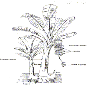
Source: Robinson and De Villier, 2007 Figure 2.1: Morphology of a banana plant

2.1.2 Ecology

Banana is cultivated principally in the tropics. The major banana-growing regions of the world are situated between the equator and latitudes 20°N and 20°S. The crop has a high water demand and is sensitive to low temperatures and wind. The principal environmental factors which affect the growth of banana are:

· Water

Availability of water is one of the critical factors that determine where bananas should be grown. It is generally considered that bananas require a weekly precipitation of 30-40 mm of rainfall or 1500-2000 mm annually for optimum growth. There is however, overwhelming evidence worldwide (except in parts of the humid tropics) to support the need for supplementing irrigation of bananas as rainfall distribution is seasonal and erratic.

With respect to the use of water, the banana plant has a number of important characteristics (Swennen and Vuysteke, 2001):

- A high evapotranspiration rate due to large broad leaves and large total surface area. Maximum evapotranspiration is estimated at between 5-6 mm/day.

- A shallow superficial root system compared with most tree-fruit crops. In general,
100 % of water is obtained from the first 0.5-0.8 m with 60 % from the first 0.3 m.

- A poor ability to withdraw water from a soil with low moisture content. A depletion of 35 % (management allowable deficit) of the total available water should thus not be exceeded.

- A rapid physiological response to soil water deficit especially in conditions of high evaporative stress. Robinson & Alberts (1987), found that, after 6 days without water, when tensiometers showed 25 kPa, the level of photosynthesis on banana plants reduced by 19 % compared with well-watered plants. When tensiometers showed 70 kPa, the level of PS was reduced by 80 %. At this stage, external wilting symptoms are clearly visible.

· Temperature

The rate of banana growth and development is determined by temperature. On the basis of the mean daily temperatures (maximum + minimum /2), the optimum mean for photosynthesis and flower initiation is 22°C, whereas the optimum mean for plant development and leaf emergence is 31°C (Turner & Lahav, 1983; Robinson & Anderson, 1991). Mean temperature balance required for growth (assimilation) and development (leaf emergence) is 27°C.

· Soils

According to Delvaux (1995), soil physical factors important for banana are porosity and mechanical impedance (compaction), aeration and natural drainage (water logging), water-holding capacity and soil temperature. Plantation longevity and sustained high production is dependent on porous, loose soils which allow unimpeded root extension. Banana root density is thus inversely related to soil bulk density. When using a penetrometer, the soil strength should not exceed 1500 kPa down to 800 mm depth. Studies in waterlogged soils, in South Africa indicate drains should be dug between rows of bananas to assist in the removal of excess water from about 12 m on both sides of the drain,

thus a deep drain every eight banana rows will be a useful insurance policy (Robinson and De Villier, 2007). Minimum soil temperatures of 10°C to 15°C are severely restricting on banana root extension. Hence, the slope aspect which conditions the field exposure to sunlight as well as the planting density will affect soil temperature.

Sandy Clay soils are best for bananas because there is a good balance between the water-holding capacity and the cation exchange capacity on the one hand, and increased aeration, water infiltration and drainage on the other hand. Optimum soil texture should be about 30% clay, 10% silt and 60% sand. The texture thus determines the total available water (TAW). The TAW is expressed in mm water/m soil depth. Light sandy soils will therefore require more frequent watering to maintain field water capacity than will do loam or clay soils.

Soil chemical aspects such as soil acidity and salinity are equally important for plant growth and in irrigation management (Robinson and De Villier, 2007). For optimum plant growth, the soil pH measured in water should be between 5.8 and 6.5. Salinity is usually only a problem in Mediterranean climates, which have saline soils, low rainfall and use poor irrigation water. Thus, soils with electrical conductivities of less than 1mmho/cm are required for good growth.

· Wind

Wind causes different types of damage in banana plantation. At wind velocities of more than 70 km/h, between 50-100% of the plants can be blown down. Winds modify the physiological functioning of the banana plant through its effect on the boundary layer of moist, undisturbed air adjacent to the leaf surface, and by its effect on leaf temperature. If the wind speed is high and humidity low, the boundary layer quickly disperses, leaf temperature rise, stomata close and the plant suffers physiological stress. Propping is usually employed in supporting banana and windbreak and hedges to prevent wind damage.

2.2 Definition of some Terms and Concepts related to Irrigation

Field Capacity (FC)

This is refers to the maximum quantity of water that the soil can hold against the forces of gravity. It corresponds to a suction of 0.1bar (Fonteh & Assoumou, 1996).

Permanent Wilting Point (PWP)

This is the moisture content at which a plant wilts permanently under conditions of water stress even if it is later placed in a saturated atmosphere. It is assumed to correspond to a suction of 15bars (Fonteh & Assoumou, 1996).

Available Water Content (AWC) and Total Available Water Content (TAWC)

This is the quantity of water that is readily available in a soil for plant growth. It is expressed as the difference between field capacity and permanent wilting point.

AWC= èfc - èwp (2.1)

The total Available Soil Water content (TAW) is defined as the difference in soil moisture content between soil field capacity (èfc) and wilting point (è_wp). It represents the ultimate amount of water available to the crop and depends on the texture, structure and organic matter content of the soil. The total available water in the root zone can be calculated as follows (Hanks and Ashcroft, 1980):

TAWC = (èfc - èwp) Z_r (2.2)

Where,

TAWC= Total available soil water in the root zone (m)

èfc = Water content at Field capacity (m³/m³)

èwp = Water content at wilting point (m³/m³)

Z_r = Root Depth (m)

Root depth growth with time can be calculated using the procedure described by Borg and Grimes (1986) and given by the equation:

Zr = Zrm [0.511 +0.511Sin (3.03 - 1.47)] (2.3)

Where,

The angle is in radians,

Zr is the root depth in cm,

Zrm is the maximum root depth of the crop in cm, DAP is the number of days after planting, and

DTM is the number of days to maximum root depth.

The root depth growth rate is 1.2 mm/day for grass and 1.5 mm/day for banana until maximum effective root depth has been reached (Plauborg et al., 1996). The maximum effective root depth is determined by both crop and soil type.

Soil Moisture Deficit (SMD)

This is the difference between field capacity and the actual soil moisture content. It is normally the depth of water that should be replaced by irrigation (Merriam & Keller,

1975).

P

eff o

Effective Rainfall

? 125

This is the fraction of precipitation that is effectively used by plants after the deduction of surface run off and deep percolation (Van Laere, 2003). The effective precipitation depends on a number of variables: amount, intensity and frequency of rainfall; evaporative demand; terrain characteristics; soil and crop; groundwater location; management practices; etc., (Kopec et al., 1984). Due to the difficulty of measuring all these variables, some authors recommend the use of empirical equations or to estimate the effective precipitation _(Peff) as a percentage of total precipitation _(Ptot). In the last case, a value of 80 % is recommended when rainfall depth is below 100 mm/month (Rojas & Rolda'n, 1996). Moon and Van der Gulik (1996) stated that the effective precipitation is ignored if it is under 5 mm/day as this amount is not likely to penetrate the soil surface and will be evaporated. The effective rainfall could equally be calculated as proposed by the United States Department of Agriculture Soil Conservation Service (Smith et al, 1996).

for Ptot < 250mm (2.4)

for Ptot > 250mm (2.5)

Readily Available Water and Depletion Factor

The fraction of total available water that a crop can extract from the root zone without suffering water stress is the readily available water (RAW). The depletion factor is the fraction of the total available soil water that can be depleted from the root zone before moisture stress occurs (P ranges from 0 to 1). The P values are expressed as a fraction of TAWC with lower values taken for sensitive crops with limited root systems under high evaporative conditions, and higher values for deep and densely rooting crops and low

evaporation rate (Doorenbos et al., 1986). At low rates of ETc, the p values are higher than at higher rates of Etc.

RAW = P * TAWC (2.6)

Where,

RAW = Readily Available Water,

P= depletion factor (0.35 for banana plants).

2.3 Evapotranspiration

One way to improve water use efficiency and optimize plant production is to provide crops only with the water they need based on the climate-plant-soil relationship. Therefore the concept of evapotranspiration (ET) is the base for the right amount of irrigation water that should be applied.

Water supplied to crops is lost from the soil through direct evaporation and transpiration into the atmosphere (Fonteh and Assoumou, 1996). It is difficult for us to isolate the two mechanisms on a field with growing crops. As such the two losses are usually combined to give evapotranspiration (ET). Knowledge of ET enables us to predict the soil moisture deficit (SMD) for irrigation. We express the ET as a rate of loss of water e.g. 5 mm/day. ET could also be referred to as the consumptive use i.e. the total amount of water a crop takes from the soil as it grows. Designs of irrigation systems are usually based on the period of the growing season with the maximum consumptive use. Systems are designed with capacities to supply water when demand is the highest. We can differentiate between two types of ET: reference crop ET and actual ET. Reference crop evapotranspiration (ET_o) is the water use of a vigorously growing reference crop under full cover, when water is not limiting (Fonteh and Assoumou, 1996). The crop or actual evapotranspiration (ET_a) is the actual amount of water lost from the soil during field growing conditions. The reference crop ET is related to the actual by the equation:

(2.7)

KC is a coefficient accounting for crop maturity and water stress under which the plant is growing. KC values vary with the crop, its stage of growth, growing season and prevailing weather conditions. From the equation (2.7) the actual ET is obtained from the reference. This is because depends only on climatic factors and hence, it is easier to obtain

and then apply the crop coefficient (KC). ET_a can be obtained directly for example, by determining the moisture content (MC) of the soil between a given time interval. However, this approach is slow and tedious and is used only as a check on indirect methods.

Table 2.1: Length of crop growth developmental stages for various planting periods and Climatic regions

	Stages of Development					Plant date		Region
								Crop characteristic
Initial	Crop Development	Mid- season	Late	Total				Banana 1^st year
	Stage length, days
120	90	120	60	390	March	Mediterranean		Depletion Coefficient, p
0.35	>>	0.35	0.35	-				Root Depth, m
0.30	>>	>>	0.80	-				Crop Coefficient, C
0.5	>>	1.1	1.0	-				Yield Response Factor, Ky
				1.2- 1.35				Banana 2nd year
	Stage length, days
120	60	180	5	365	February	Mediterranian		Depletion Coefficient, p
0.35	>>	0.35	0.35	-				Root Depth, m
0.30	>>	>>	0.8	-				Crop Coefficient, C
1.0	>>	1.2	1.1	-				Yield Response Factor, Ky
				1.2- 1.35

Source: Allen et al., 1998

Table 2.2: Monthly K_c values of Banana for tropical climate

Months after planting KC		Crop Developmental Stage
		2	3	4	5	6	7	8	9	10	11	12	13	14	15
		0.4	0.45	0.5	0.6	.7	0.85	1.0	1.1	1.1	0.9	0.8	0.8	0.95	1.05
		shooting						Harvesting

Source: Allen et al., 1998

2.3.1 Measurement of evapotranspiration

ET is not easy to measure. Specific devices and accurate measurements of various physical parameters or the soil water balance in Lysimeters are required to determine ET (Allen et al., 1998). The methods are often expensive, demanding in terms of accuracy of measurement and can only be fully exploited by well-trained research personnel. Although the methods are inappropriate for routine measurements, they remain important for the evaluation of ET estimates obtained by more indirect methods. The methods used in the measurement of ET are: Energy balance and Microclimatological methods, Soil water balance, Lysimeters, Meteorological data, Pan Evaporation. Owing to the difficulty of obtaining accurate field measurements, ET is commonly computed from weather data. A large number of empirical or semi-empirical equations have been developed for assessing crop or reference crop ET from meteorological data. Some of the methods are only valid under specific climatic and agronomic conditions and cannot be applied under conditions different from those under which they were originally developed.

Numerous researchers have analyzed the performance of the various calculation methods for different location. As a result of an Expert Consultation to compare several methods of calculation of ET_o in May 1990, the FAO Penman-Montheith method is now recommended as the standard method for the definition and computation of reference evapotranspiration, ET_o (Allen et al., 1998)

2.3.2 The Penman-Montheith equation

In 1948, Penman combined the energy balance with the mass transfer method and derived an equation to compute the evaporation from an open water surface from standard climatological records of sunshine, temperature, humidity and wind speed (Allen et al.,

1998). This so-called combination method was further developed by many researchers and extended to cropped surfaces by introducing resistance factors.

From the original Penman-Montheith equation and the equations of the aerodynamic and surface resistance, the FAO Penman-Montheith method to estimate ET_o is:

(2.8)

Where,

ET_o reference ET [mmday^-1],

R_n net radiation at the crop surface [MJm^-2day^-1],

G soil heat flux density [MJm^-2day ^-1],

T mean daily air temperature at 2 m height [^oC],

U2 wind speed at 2 m height [ms^-1],

e_s saturation vapor pressure [KPa],

e_a actual vapor pressure [KPa],

(e_s - e_a) represents the vapor pressure deficit of the air [KPa],

ñ_a is the mean air density at constant pressure,

cp is the specific heat of the air,

Ä represents the slope of the saturation vapor pressure temperature relationship, ã is the psychometric constant,

The equation uses standard climatological data of solar radiation (sunshine hours), air temperature, humidity and wind speed. To ensure the integrity of computations the weather data should be collected at 2 m above the extensive surface of green grass, shading the ground and not short of water.

2.3.3 Meteorological factors determining evapotranspiration

The meteorological factors determining ET are weather parameters which provide energy for vaporization and remove water vapor from the evaporating surface (Allen et al., 1998). The principal weather parameters to consider are:

· Solar radiation

The ET process is determined by the amount of energy available to vaporize water. Solar radiation is the largest energy source and is able to change large quantities of liquid water into water vapor. The potential amount of radiation that can reach the evaporating surface is determined by its location and time of the year. Due to differences in the position of the sun, the potential radiation differs at various latitudes and in different seasons. The actual solar radiation reaching the evaporating surface depends on the turbidity of the atmosphere and the presence of clouds, which reflect and absorb major parts of the radiation. Not all-available energy is used to vaporize water part is used to heat up the atmosphere and soil profile.

· Air temperature

The solar radiation absorbed by the atmosphere and heat emitted by the earth increase the air temperature. The sensible heat of the surrounding air transfers energy to the crop and exerts as such a controlling influence on the rate of evaporation. In sunny warm weather, the loss of water by ET is greater than cloudy and cool weather.

· Air humidity

While the energy supply from the sun and surrounding air is the main driving force for the vaporization of water, the difference between the water vapor pressure at the evapotranspiring surface and the surrounding air is the determining factor for the vapor removal. Well-watered fields in hot dry arid regions consume large amount of water due to the abundance of energy and the desiccating power of the atmosphere. In humid tropical regions, notwithstanding the high-energy input, the high humidity of the air will reduce the ET demand. In such an environment the air is already close to saturation, so that less additional water can be stored and hence the ET rate is lower than in arid regions.

· Wind speed

The process of vapor removal depends largely on wind and air turbulence, which transfer large quantities of air over the evaporating surface. When vaporizing water, the air above the evaporating surface gradually becomes saturated with water vapor. If this air which is the driving force for water vapor removal is not continuously replaced with drier air ET rate decreases.

2.4 Maximum Production

Banana cultivation is mainly geared towards the production of fruits, for the production of beer, animal feeds and not the least the production of fibers for textile industry (Marty, 1983). In this study, the objective of banana cultivation is for the production of fruits. Many models to estimate the potential production of crops have been developed. Doorenbos et al., (1986) presented the Dewit model in 1965 as a model of estimation of the potential production of crops. This model unfortunately has not yet been adopted for the banana crop surely due to the complexity of this perennial herbaceous plant. Smith et al., (1996) concluded that agricultural production is affected by the level of water stress that will be experienced by the crops during development. This model goes from

E

linear regression, to bring in the rate of production reduction to arrive at a relation that

? 1 ?

? E x

Smith et al (1996) called Crop Water Yield Function? (CWYF). The summarized equation is as follows:

(2.9)

In this equation Y_a is the actual production in tons/hectare (t/ha); _Ymax is the maximum production in t/ha; ET_a is the actual evapotranspiration in mm/season; _ETmax is the maximum evapotranspiration in mm/season and K_y is the yield response factor and has no unit. K_y describes the reduction in relative yield due to water stress. Doorenbos et al., (1986) suggested that for banana, K_y will have a value between 1.2 and 1.35,

represents the rate of evapotranspiration reduction, and

represents the rate of production reduction due to water stress

The problem with this model is the determination of the maximum production of a banana plantation with respect to only the response to water, indifferently from other factors of production such as soil factors, crop factors, climate and topography.

Beernaert and Bitondo (1993) in their effort to consider many factors for the estimation of the potential production of crops presented a model called Modèle d`évaluation des terres?. This model considers factors such as winds, fungus or nematodes diseases, the crop species cultivated and others, and is more reliable than other models.

They have used this model on many crops including banana. They estimate that in ideal conditions (without limitations) the potential production of a banana plantation ranges between 40 and 60 tons/ha.

2.5 Pressurized Irrigation Systems 2.5.1 Sprinkler irrigation systems

Sprinkler irrigation is a versatile means of applying water to any crop, soil, and topographic condition (Schwab et al., 1993; Fonteh and Assoumou, 1996). Sprinkler systems can be efficient on soils and topography that is not suitable or efficient for surface irrigation methods. In general, systems are described according to the method of moving the lateral lines on which various types of sprinklers are attached. Laterals may be stationary or movable. Sprinkler systems are highly efficient but there are general concerns about the maintenance and investment costs for these systems.

Hand-moved laterals have the lowest investment cost but the highest labour requirement. These systems are only suitable for short growing crops.

The side roll lateral system uses the irrigation pipe as the axle of large diameter wheels that are spaced about 12 m apart. These laterals are moved by a gasoline powered motor and thus require less labor than hand-move systems. Side rolls should be used for crops that will not interfere with the movement of the lateral or sprinkler pattern.

Centre pivots consist of radial pipelines that rotate around a central pivot by water pressure, electric motors, or oil hydraulic motors (Schwab et al., 1993). A variety of nozzle types, nozzle heights, and application rates can be used in centre pivot systems. Sprinkler systems are selected according to the field conditions for the most efficient operation.

Linear moved laterals use hardware similar to that of a centre pivot, but move in a straight line across the field. Solid-set systems have sprinklers that are placed over the entire field, where all or some of the sprinklers may operate at the same time. Sprinkler heads vary greatly from older impact heads to more modern spray heads that have an assortment of application and placement modes (Howell, 2003).

2.5.2 Micro irrigation systems

Micro irrigation is a method for delivering slow, frequent applications of water to the soil using a low pressure, low volume distribution system and special flow-control outlets (Schwab et al., 1993). If managed properly, micro irrigation can increase yields and decrease water, fertilizer, and labor requirements. Micro irrigation includes: micro sprinklers, drip irrigation, and subsurface drip irrigation (SDI).

Micro sprinklers, often referred to as micro sprayers or misters, typically consist of small emitters placed on short risers above the soil surface. Water is conveyed through the air, but travels only a short distance before reaching the soil surface. The wetted area of emitters in these systems is small, can be controlled fairly easily, and has different shapes to match desired distribution patterns. The advantages of micro sprinkler irrigation systems are the potential for controlling frost, greater flexibility in applying water, and lower susceptibility to clogging.

Drip systems deliver water directly to the soil surface or subsurface (SDI) and allow water to dissipate under low pressure in a predetermined pattern. These systems are advantageous because water is applied directly to or just above the root zone of the plant, thereby minimizing deep percolation losses, reducing or eliminating the wetted area from which water can evaporate, and eliminating losses associated with runoff. These systems are also advantageous because they reduce water consumption by weeds, while operating at a lower pressure.

Micro irrigation systems apply water on a high-frequency basis and create near optimal soil moisture conditions for the crop. Under proper management, micro irrigation systems save water because only the plant`s root zone is supplied with water and little, if any, is lost to deep percolation, consumption by non beneficial plants, or soil surface evaporation. In addition to being highly efficient, these systems also require relatively little labour input if designed properly. Yields of some crops have been shown to increase under these systems because the high temporal soil water level needed to meet transpiration requirements is maintained (Colaizzi et al., 2003).

The major disadvantages of micro irrigation systems are high initial cost and potential for the emitters clogging. In some cases, labor inputs may be quite high if rodents

burrow and chew system components. Proper design, operation, and maintenance can overcome many of these issues.

2.6 Irrigation Scheduling and Management 2.6.1 Irrigation management

Irrigation management can be defined as the process of implementation of suitable operation and maintenance in order to meet the objectives of the concerned irrigation system and monitoring of the activities to assure that the objectives are met.

Three implications can be drawn from the above definition. First of all, that irrigation management is not a routine job. The management decisions have to be made with great care, as they have to match with the operation and maintenance objectives. Secondly, even though the overall goal may be the same, objectives vary from system to system, hence management decisions have to take account of these inter system differences. Thirdly, that monitoring is an integral part of management thus management decisions have to be continuously refined according to the feedback obtained from monitoring and evaluation.

Irrigation Management is one of the major challenges for the irrigation professionals. It is important as it decides the benefit derived from the irrigation system.

2.6.2 Irrigation scheduling

Irrigation performance can be improved either by means of developing new application systems (drip, sprinkler, etc.) or by a more accurate irrigation scheduling. For any crop, schedule implies the determination of time and volume of water application to meet a specified management objective.

Jensen (1981) defines irrigation scheduling as a planning and decision-making activity that the farm manager or operator of an irrigation farm is involved in before and during most of the growing season for each crop that is grown. It could also be defined as the use of water management strategies to prevent over application of water while minimizing yield loss due to water shortage or drought stress. He further indicated four types of data needed for irrigation decision making:

1) Current level and expected change in available soil water for each field over the next 5 to 10 days.

2) Current estimates of the probable latest date of the next irrigation on each field to avoid adverse effects of plant water stress.

3) The amount of water that should be applied to each field, which will achieve high irrigation efficiency.

4) Some indication of the adverse effects of irrigation a few days early or late.

Irrigation scheduling requires a particular attention because of its influence on irrigation efficiency and its consequences on the environment. The water holding capacity of the soil and the suction that the cultivated crop can develop on the soil water are good guides for irrigation scheduling. The techniques used currently for irrigation scheduling are diverse. Relative to the equipments that are used for these techniques, they can be sophisticated or very simple. Methods based on direct measurements of plant water status have always attracted the attention of irrigation research as a tool for irrigation timing, but getting accurate and representative data for these parameters has always been very difficult (Cremona et al., 2000). Based on the soil-plant-water relations, Kramer (1983) suggested that the determination of the time and quantity of water to supply by irrigation could be obtained by either one of the three fundamental methods namely:

· Determination of soil moisture

· Estimation of the water used by plants from climatic data

· Measure of water stress that has affected the crop

Irrigation scheduling to satisfy the water requirement of plants must conform to the hydrology of the milieu and to the objectives set by the irrigation practice. Njila (1999), stated that most irrigation managers in Cameroon prefer to irrigate their crops following a pre-established calendar.

Whatever the context, Fonteh & Assoumou (1996), Tron et al. (2000), present two fundamental questions that need to be answered in any irrigation scheduling program:

- When to irrigate?

- How much water to apply?

Smith et al, (1996) classified scheduling options into two different categories as follows:

a) Timing options - related to when irrigation is to be applied:

1) Each irrigation defined by user; this type is used to evaluate irrigation practices and to simulate any alternative irrigation schedule.

2) Irrigation at critical depletion (100 % depletion of readily available soil moisture). Resulting in minimum irrigations, but irregular and therefore unpractical irrigation intervals.

3) Irrigation below or above critical depletion (% depletion of readily available soil moisture). Useful to set a safety level above critical soil moisture or allow a critical stress level.

4) Irrigation at fixed intervals per stage, suitable in particular in a gravity system with rotational water distribution, may result in some over-irrigation in the initial stages and under-irrigation in the peak season.

5) Irrigation at given crop evapotranspiration reduction (%).

6) Irrigation at given yield reduction (%).

7) No irrigation, only rainfall.

b) Application options - how much water is to be given per irrigation turn:

1) Each irrigation depth is defined by the user, as determined from field or simulated data.

2) Refill soil to field capacity, to bring soil moisture content back to field capacity, thus equal to the depleted soil moisture in the root zone, as the depletion in the root zone will normally vary over the growing season with changing root depth and allowable depletion levels.

3) Refill below or above field capacity. Useful to allow for leaching for salinity control

(above field capacity) or to accommodate possible rainfall (below field capacity).

Irrigation scheduling schemes should take into account factors such as the soil properties that affect soil moisture-holding capacity. James et al. (1982) for example, reported that irrigation scheduling with a soil of low water-holding capacity would have to be more frequent with smaller amounts applied each time for best efficiency.

2.6.3 Importance of irrigation scheduling

Some irrigation water is stored in the soil to be removed by crops and some is lost by evaporation, runoff, or seepage. The amount of water lost through these processes is affected by irrigation system design and irrigation management. Prudent scheduling minimizes runoff and percolation losses, which in turn usually maximizes irrigation efficiency by reducing energy and water use.

Energy can thus be saved by no longer pumping water that was previously being wasted. When water supplies and irrigation equipment are adequate, irrigators tend to over irrigate, believing that applying more water will increase crop yields. Instead, over irrigation can reduce yields because the excess soil moisture often results in plant disease, nutrient leaching, and reduced pesticide effectiveness. In addition, water and energy are wasted.

The quantity of water pumped can often be reduced without reducing yield. Studies have shown that irrigation scheduling using water balance methods can save 15 to 35 percent of the water normally pumped without reducing yield (Evans et al., 1996). Maximum yield usually does not equate to maximum profit. The optimum economic yield is less than the maximum potential yield. Irrigation scheduling tips presented in popular farm magazines too often aim at achieving maximum yield with too little emphasis on water and energy use efficiencies. An optimum irrigation schedule maximizes profit and optimizes water and energy use.

2.7 Geographic Information Systems

A geographic information system (GIS), or geographical information system is a system which captures, stores, analyzes, manages, and presents data that is linked to location (Chang, 2007). GIS provides a means of measuring spatial and attribute data into a computerized database system, thereby allowing input, storage, retrieval and analysis of geographically referenced data (Heywood et al., 2006). It is therefore a system of computer hardware, software, and procedures designed to support the capture, management, manipulation, analysis, modeling, and display of spatially referenced data for solving complex planning and management problems. In the strictest sense, the term describes any information system that integrates stores, edits, analyzes, shares, and displays geographic

information. In a more generic sense, GIS applications are tools that allow users to create interactive queries (user created searches), analyze spatial information, edit data, maps, and present the results of all these operations. Analyzing large amount of data is a necessity for management of irrigation projects. Data must be collected, stored and interrelated with each other in such a way that the data are readily accessible (Dayyani et al., 2003). The cartographic and data overlaying capability of GIS coupled with its dynamic linking ability to models plays a vital role in water management. In addition, its ability of writing scripts gives the decision makers this power to produce the necessary outputs the way they need them.

GIS technology can be used for water resource management, asset management, archaeology, environmental impact assessment, urban planning, cartography, criminology, geographic history, marketing, logistics, scientific investigations, prospectivity mapping, and other purposes. For irrigation management adequate and updated information regarding the irrigation system is needed, thus GIS tool for irrigation management provides information interactively for decision making process. GIS have the capability of improving water management techniques as well as decision-making (Taylor, 2005). GIS have thus, taken a central role in analyzing, modeling, and managing a wide range of water resource information. System GIS can analyze spatial interactions between static and dynamic entities.

1. Spatial data management

2. Interactive visualization

3. Spatial analysis

4. Customization and decision-making support.

The importance of spatial geographic components in on-farm irrigation system performance imposes the involvement of the capabilities to be able to store, aggregate, manipulate, analyze and visualize a huge quantity of data. In the recent last ten years, to this purpose, the use of GIS has been greatly diffused. These systems, if combined to appropriate simulation models could support the decisions of designers and/or managers (Hoogenboom et al., 1991).

A GIS is characterized by a unique ability of the user to overlay spatial layers, each, representing one or more physical and/or functional characteristics of the studied

phenomenon. Each layer is related to a table, representing the database. Using appropriate models, it is then possible to actively elaborate the information and to present results under tabular and/or maps form.

There have been several applications of GIS in irrigation and drainage systems around the world. Sarangi et al., (2001) used GIS in development of input data set for a conceptual small watershed runoff generation model. In addition, they used ARC/INFO for canal system within the project area of Patna Canal and distributaries of Sone command area in India. Amor et al., (2002) combined GIS with a crop growth model to estimate the water productivity in time and space in the Philippines. Three products, rice, corn and peanut were modeled in their research. They analyzed the water limitation for each crop in different seasons and determined the productivity potential in the region. In Iran, application of GIS dates as far back as the 90's in diverse fields of water sciences such as hydrology, flood control, water erosion, and groundwater management. Daneshkar et al. (2000) used GIS and Modflow for simulation of Ab-Barik groundwater plain. Alvankar et al. (2000) applied GIS in watershed characterization of the Latvian dam watershed.

2.7.1 Data acquisition and representation

GIS data represents real world objects (roads, land use, elevation) with digital data. Real world objects can be divided into two abstractions: discrete objects (a house) and continuous fields (rain fall amount or elevation). There are two broad methods used to store data in a GIS for both abstractions: Raster and Vector.

a) Raster data

A raster data type is, in essence, any type of digital image represented in grids. While a digital image is concerned with the output as representation of reality, in a photograph or art transferred to computer, the raster data type will reflect an abstraction of reality. Aerial photos are one commonly used form of raster data, with only one purpose, to display a detailed image on a map or for the purposes of digitization. Other raster data sets will contain information regarding elevation or reflectance of a particular wavelength of light.

Raster data type consists of rows and columns of cells, with each cell storing a single value. Raster data can be images (raster images) with each pixel (or cell) containing a color value. Additional values recorded for each cell may be a discrete value, such as land

use, a continuous value, such as temperature, or a null value if no data is available. While a raster cell stores a single value, it can be extended by using raster bands to represent RGB (red, green, blue) colors, color maps (a mapping between a thematic code and RGB value), or an extended attribute table with one row for each unique cell value. The resolution of the raster data set is its cell width in ground units. Raster data is stored in various formats; from a standard file-based structure of Tagged Image File (TIF), Joint Photographic Experts Group (JPEG), etc. to binary large object (BLOB) data stored directly in a relational database management system (RDBMS) similar to other vector-based feature classes. Database storage, when properly indexed, allows for quicker retrieval of the raster data but can require storage of millions of significantly-sized records.

b) Vector data

In a GIS, geographical features are often expressed as vectors, by considering those features as geometrical shapes. Different geographical features are expressed by different types of geometry:

· Points

Zero-dimensional points are used for geographical features that can best be expressed by a single point reference; in other words, simple location. Points can also be used to represent areas when displayed at a small scale. For example, cities on a map of the world would be represented by points rather than polygons. No measurements are possible with point features.

· Lines or polylines

One-dimensional lines or polylines are used for linear features such as rivers, roads, railroads, trails, and topographic lines. Again, as with point features, linear features displayed at a small scale will be represented as linear features rather than as a polygon. Line features can measure distance.

· Polygons

Two-dimensional polygons are used for geographical features that cover a particular area of the earth's surface. Such features may include lakes, park boundaries, buildings, city boundaries, or land uses. Polygons convey the most amount of information of the file types. Polygon features can measure perimeter and area.

Each of these geometries is linked to a row in a database that describes their attributes. For example, a database that describes water resource may contain its depth, water quality, pollution level. This information can be used to make a map to describe a particular attribute of the dataset. For example, water resources could be colored depending on level of pollution. Different geometries can also be compared.

Vector features can be made to respect spatial integrity through the application of topology rules such as 'polygons must not overlap'. Vector data can also be used to represent continuously varying phenomena. Contour lines and triangulated irregular networks (TIN) are used to represent elevation or other continuously changing values. TINs record values at point locations, which are connected by lines to form an irregular mesh of triangles. The faces of the triangles represent the terrain surface.

2.7.2 Advantages and disadvantages of vector and raster data

There are advantages and disadvantages to using a raster or vector data model to represent reality.

Raster datasets record a value for all points in the area covered which may require more storage space than representing data in a vector format that can store data only where needed. Raster data also allows easy implementation of overlay operations, which are more difficult with vector data.

Vector data can be displayed as vector graphics used on traditional maps, whereas raster data will appear as an image that, depending on the resolution of the raster file, may have a blocky appearance for object boundaries.

Vector data can be easier to register, scale, and re-project. This can simplify combining vector layers from different sources. Vector data is more compatible with relational database environments. They can be part of a relational table as a normal column and processed using a multitude of operators.

The file size for vector data is usually much smaller for storage and sharing than raster data. Image of raster data can be 10 to 100 times larger than vector data depending on the resolution. Another advantage of vector data is that it is easy to update and maintain.

2.7.3 Steps used for the putting in place of a GIS project

In a typical GIS project, there is need to identify the objectives of the project, create a database specifically for the project and containing all information for the resolution of the problem, then, we need to use GIS functions to create an analytical model that will be able to solve the problem and lastly present the results of the analysis. ESRI (1996), define four basic steps in the development of a GIS project.

Step 1: Identification of objectives

The first step of the procedure consists in identifying the objective of the analysis. The following questions need to be taken into consideration in order to define the objectives:

· What is the problem to be solved? How is the problem being solved actually? Are there any more solutions with the aid of GIS?

· What are the expected results: reports, study maps, presentation maps?

· To whom are the results destined: management, technicians?

· Are the data going to be used for other goals? What are the conditions in this case?

This is an important step as the answers to the latter questions define the objectives of the project as well as the methods to be used in putting in place the system.

Step 2: Creation of a database

The second step consists of creating a database for the project. The creation of this database is a three stage procedure. The stages help in the conception of the database, to automate and to assemble the data and then manage this data. The design of a database comprises:

· The identification of the necessary spatial data with respect to the need in analysis, definition of the different attributes required by the various entities, definition of the boundaries of the study area and the choice of the coordinate system to be used,

· Automating access to the data which comprises the digitization or the conversion of data from other systems and formats to a useable format, as well as the verification of the data and correction for errors, and

· Management of the data which comprises the verification of the coordinate system and union of two adjacent layers.

Creation of a database for the project is of prime importance and usually takes a greater part of the time required for a GIS project. The completeness and precision of the data used in analyses will equally determine the precision of the results. This explains why this study is centered towards the creation of a database for the irrigation system of the PHP group.

Step 3: Data analysis

This third step consists of analyzing the data obtained. Analysis of GIS moves from simple realization of maps to the creation of complex spatial models. A model is the representation of reality used to simulate a given process, predict a given result or analyze a given problem. A spatial model applies one or more of these three categories of functions of GIS:

· Geometric modeling - calculation of distances, areas and perimeters, creation of buffer zones,

· Coincidence modeling - superposition of various data to find their locations or the coinciding values,

· Contiguity modeling- allocation, search for routes and cutting into sectors.

With the use of GIS it is possible to carry out rapid analysis which would have been extremely long or even impossible to do manually. Different scenarios are being created by changing the method or a parameter of an event and executing the analysis to obtain various results.

Step 4: Presentation of Results

This is the final stage of a GIS project. In most cases, GIS results are better shown on maps. Diagrams and data reports are equally other methods of presenting results. These diagrams and reports could be printed separately, incorporated into created files or placed on maps.

2.8 Databases

A Database is a structured collection of data that is managed to meet the needs of a community of users (Chang, 2007). The structure is achieved by organizing the data according to a database model. The model in most common use today is the relational model. Other models such as the hierarchical model and the network model use a more

explicit representation of relationships. A computer database relies upon software to organize the storage of data. This is defined as database management system (DBMS). Some terms whose meaning is required to understand databases are (Chang, 2007):

· File

A file is an ordered arrangement of records in which each record is stored in a unique identifiable location. The sequence of the record is then the means by which the record will be located. In most computer systems, the sequence of records is either alphabetic or numeric based on field common to all records such as name or number.

· Records

A record or tuple is a complete set of related fields. For example, Table 2.3 shows a set of related fields, which is a record. In other words, if this were to be a part of a table then we would call it a row of data. Therefore, a row of data is also a record.

Table 2.3: Set of related fields in an irrigation system which form a record

Id_plot #laterals #sprinklers Flow rate			Field Record	Nyombe 255 445 250

· Field

A field is a property or a characteristic that holds some piece of information about an entity. Also, it is a category of information within a set of records. For example, the first names, or address or phone numbers of people listed in address book.

· Relations

In the relational data model, the data in a database is organized in relations. A relation is synonymous with a =table`. A table consists of columns and rows, which are referred as field and records in DBMS terms, and attributes and tuples in Relational DBMS terms. A comparison between DBMS and RDBMS terms is given in Table 2.4.

· Attributes

An attribute is a property or characteristics that hold some information about an entity. An irrigation network for example starts from a pumping station which has attributes such as a name, given number of pumps and engines etc.

Table 2.4: Comparing DBMS and Relational DBMS (RDBMS) terms

Common Term DBMS Terminology RDBMS Terminology

Database Table Database

Table Table Relation

Column Field Attribute

Row Record Tuple

2.8.1 Database management systems

A Database Management System (DBMS) is a set of computer programs that control the creation, maintenance, and the use of the database of an organization and its end users (Codd, 1970). It controls the organization, storage, management, and retrieval of data in a database. DBMS are categorized according to their data structures or types, sometime DBMS is also known as database manager. It is a set of prewritten programs that are used to store, update and retrieve a database. A DBMS includes:

- A modeling language to define the scheme of each database hosted in the DBMS, according to the DBMS data model.

- Data structures (fields, records, files and objects) optimized to deal with very large amounts of data stored on a permanent data storage device (which implies relatively slow access compared to volatile main memory).

- A database query language and report writer to allow users to interactively interrogate the database, analyze its data and update it according to the users privileges on data.

The four most common types of organizations are the hierarchical, network, relational and object models. Inverted lists and other methods are also used. A given database management system may provide one or more of the four models. The optimal structure depends on the natural organization of the application's data, and on the application's requirements (which include transaction rate (speed), reliability, maintainability, scalability, and cost).

Some DBMS software include Microsoft Access, Oracle DB2, Sybase Adaptive Server Enterprise, FileMaker Firebird, INGRES, Informix, Microsoft SQL Server, Microsoft

Visual FoxPro, MySQL, PostgreSQL, Progress, SQLite, Teradata, CSQL, OpenLink Virtuoso.

Some benefits obtained from the use of DBMS could include:

· Improved strategic use of corporate data,

· Reduced complexity of the organization`s information systems environment,

· Reduced data redundancy and inconsistency,

· Enhanced data integrity,

· Application-data independence,

· Improved security,

· Improved flexibility of information systems,

· Increased access and availability of data and information,

· Logical & physical data independence,

· Concurrent access anomalies,

· Facilitate atomicity problem,

· Provides central control on the system through database applications.

2.8.2 Relational databases

A short definition of a RDBMS may be a DBMS in which data is stored in the form of tables and the relationship among the data is also stored in the form of tables (Codd, 1970). Data items are organized as a set of formally-described tables from which data can be accessed or reassembled in many different ways without having to reorganize the database tables.

The relational model is the most commonly used today. It is used by mainframe, midrange and microcomputer systems. It uses two-dimensional rows and columns to store data. The tables of records can be connected by common key values. There are 3 relationship types:

One-to-one (1:1) - Each record in Table A can have only one matching record in Table B and each record in Table B can be related to only one record in Table A as shown in figure 2.2. This type of relationship is not frequently used in database systems, but it can be very useful way to link two tables together. However, the information related in this way could be in one table. They may be used to divide a table with many fields in order to isolate part

of a table for security reasons, or to store information that applies only to a subset of the main table, or for efficient use of space. A one-to-one relationship is created if both of the related fields are primary keys or have unique indexes.

Table A Table B

1

1

irrigation plot

Id irrigation Plot
id plot valve
id_irrigation_system
number of
sprinklers
plot name

Plot valve

Id plot valve
Longitude
latitude
Altitude

Figure 2.2: One-to-one relationship of databases

This shows that, one irrigation plot could have one and only one valve for the control of the flow of water in the plot.

One-to-many (1:M) - It is the most common type of relationship and it is used to relate one record from the 'primary' table with many records in the 'related' table. In a one-tomany relationship, a record ('parent') in Table B can have many matching records ('children') in Table A, but a record ('child') in Table A has only one matching record ('parent') in Table B as shown in Figure 2.3. This kind of relationship is created if only one of the related fields is a primary key or has a unique index.

Table A Table B

Production plot

n 1

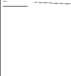
Plot name Id_production sector Soil type

Crop variety Planting date Agronomic state Spatial arrangement Irrigation plots

Total surface area slope

Name_station

Production sector

Id_production sector Surface area Id_plantation

Figure 2.3: One-to-many relation of databases

From Figure 2.3 it could be seen that, one production sector could be related to many production plots, but one production plot belongs to one and only one production sector.

Many-to-many (M:M) - is used to relate many records in the Table A with many records in the Table B. A record ('parent') in Table A can have many matching records ('children') in Table B, and a record ('child') in Table B can have many matching records ('parents') in Table A. By breaking it into two one-to-many relationships and creating a new (junction/link) table to stand between the two existing tables will enable correct and appropriate relationship setting. A many-to-many relationship is really two one-to-many relationships with a junction/link table.

A production plot for example could have many soil types and this soil type could be found in many other production plots around the plantation.

CHAPTER III
MATERIALS AND METHODS

3.1 Description of the Study Area and Experimental Site 3.1.1 Geographical Location

Njombé covers a surface area of about 260 km² and is located between latitudes 4°30`N and 4°40`N and longitudes 9°30`E and 9°45`E. The average altitude of the area is 140 m. Njombé is bounded:

· to the North by Penja,

· to the South by Mbanga,

· to the West by Tombel,

· and to the East by the Nkam.

Figure 3.1 provides the geographical location of Njombé while Figure 3.2 shows the area cultivated.

PHP group cultivates bananas and pineapples on a surface area of about 3 500 ha and is divided into plantations, with one of them being the Njombé plantation. These plantations in Njombé are an integral part of the zone of production of PHP. In 2004, the cultivated land was about 2250 ha (Boa, 2005). The plantations are further divided into sectors and the sectors into production plots.

3.1.2 Relief

Njombé has a relatively flat topography, made up of plateaus and some eroded undulating landscape. One could notice the effects of an old volcanic activity in the area (Tchiadje 1995).

3.1.3 Hydrology

The area has numerous water bodies and most of them are exploited by the companies present in the area such as PHP, Tangui, SPM and by the peasants for their day-to day activities. The principal water bodies are: the Moungo, Moulinkam, Moumbé, Bwale, Mbomé, and Ngomba.

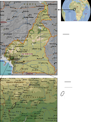
Scale :

1/20000000 Source : Encarta 2008

Scale :

1/1000000 Source : Encarta 2008

PHP plantations

Figure 3.1: Geographical location of Njombé

N

R

B

KEY

C

C: Hill

P

B: PHP cultivation

plots

P: Penja town

R: National road n°2

N: Njombe town Scale: 1/14000 Source: Google Earth version 5

Figure 3.2: Aerial view of PHP cultivation areas in the Njombé Plantations

3.1.5 Vegetation

Njombé is situated in the Guineo - Congolese floristic region, in the dense humid forest sector of the biafran forest. This forest constitutes plants of the Cesalpiniaceae family. Some of the most characteristic trees species found in the area are: Bidou (Saccaglottis gabonensis) and Azobe (Lophira alata) (Van de Pol et al, 2005). Due to the high fertility of soils in this area, there has been serious deforestation for the setting up of either large plantations or small farms or for the building of houses due to rapid urbanization. Nevertheless, one could still notice some forest reserves rich in timber and other forest species.

3.1.6 Climate

The climate of the area is equatorial with a long rainy season which runs from March to November and a short dry season which runs from November to February. It is a hot and humid climate with temperatures of 25-30°C and an average relative humidity of 80%. The cumulative average annual potential evapotranspiration equals 1 055.6mm (an average weekly ETo of 20.3mm) while the annual rainfall averages about 2550mm (Thome, 2007). Table 3.1 shows the average annual precipitation of Njombé for a 5 year period (2004-2008).

Table 3.1: Average annual precipitation of Njombé (2004-2008)

Year	Precipitation (mm)
2004	2320
2005	2385
2006	2445
2007	2960
2008	2636
Mean	2550

Source: Climatic data from PHP meteorological stations

Figure 3.3 shows the ombrothermic graph for Njombé area for the year 2008. The graph shows the rainfall amounts and evapotranspiration for the area for each week of the year and could be used to determine the start and the end of the rainy and dry seasons. The peak of the rainfall lies between the 26^th and 29^th month and almost zero from the 47^th week to the 8^th week of the year.

Figure 3.3: Monthly rainfall histogram for Njombé in 2008 3.1.7 Soils

The soils in the area are mostly ferralitic in nature. These are shallow soils with a clayey-sand granulometry. The pH of these soils varies between 4.5 and 6.5. They are thus very fertile soils, rich in mineral content. According to Defo and Marie, (1998), the soils in the banana areas of the Moungo which are of volcanic origin have undergone several studies. These studies have helped to distinguish with respect to the level of weathering of the bedding rock. We could thus distinguish three types of soils:

1) Recent soils: These are andosols dominated by allophones. These soils are characterized by a high porosity, a llight silty texture, a fragile granular structure and an important number of stones.

2)

Soils dominated by Halloysites: These soils have a silty-clay texture with a

ETP (m)

stable granular structure.

m

3) Highly weathered soils: These soils are dominated by halloysites and kaolinite. They are thus soils with high clay content and thus possess drainage problems.

3.2 Description of the Irrigation System at the PHP Group

4 0 16 9 2 2 28 3 3 40 43

The irrigation system at the PHP Group, Njombé is divided into three main parts; the pumping stations, the conduits (pipes), and the distribution network. To develop the

database for the system, a clear knowledge of how the system looks like and how it functions will be of great necessity.

3.2.1 Pumping station

The entire network is supplied through five pumping stations (Koumbe 1, Koumbe 2, Koumbe 3, Trou Lac Dia-Dia and Maya) and use 21 pumps for the lifting of water; 16 of the pumps are situated at the main station at Koumbe and 5 others situated at Trou Lac, Dia-Dia and Maya. The engine pumps used have the following characteristics:

Engine Type: 12 cylinder engine

Engine Power: 337 hp

Pump Type: Centrifugal with 5 wheels of diameters 330 mm rotating at 1800 rpm Pump Flow Rate: 240 m³/h

Total Head: 240 m

Operating Pressures: 24 bars (Koumbe) and 13-17 bars (others)

Water is pumped from the rivers Moumbe, Mboko and Maya as well as the Dia Dia Lake and Well (about 50 m deep).

3.2.2 The main line (Pipes)

Water is transported from the pumping stations to the plantation via steel or PVC pipes with diameters between 200 mm and 700 mm. These pipes are either buried, placed on the surface or have become exposed to the surface due to erosion. Interconnection between the pipes gives a looped network such that in case of malfunctioning of one of the pumping stations, the others could be used for pumping. During the irrigation season, each pipe operates individually, hence, forming a ramified network. These ramified networks cover a total distance of about 55 km and each is equipped with a given set of structures and equipments, which facilitate the use and management of these networks. Figure 3.4 shows these main conduit and the pumping stations from which they obtain water.

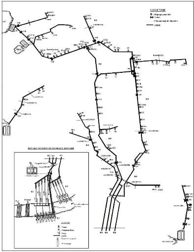
Source: Irrigation department PHP

Figure 3.4: Main lines at the PHP group

3.2.3 Distribution network

This is the set of equipment and structures which transport water from the main hydrant to the level of the sprinklers. It is made up of:

- Secondary conduits in galvanized steel or polyethylene and with diameters of 120 mm, 150 mm, or 160 mm,

- Tertiary conduits or antenna with diameters of 120 mm,

- Quaternary conduits with diameters of 40 mm or 50 mm,

- Risers and sprinklers.

This network is characterized by two main irrigation systems; overhead and Undertree:

a) Overhead irrigation

In this type of irrigation, the sprinklers are situated above the banana plants. This mode could either be by total coverage with big guns or by integral coverage with sprinklers.

· Total coverage with big guns

It is the most ancient system used by the Group and usually gives the ground base for the installation of other systems. It occupies a surface area of about 410.20 ha. The big guns used are characterized by a flow rate of 60 m³/h, an operating pressure of 5.5 bars, a horizontal throw of 54.4m, coverage of 0.5 ha/canon, and an irrigation depth of 10mm/h. the number of big guns per irrigation plot is between 60-100 big guns, this gives a spacing of 72 or 78 m in the line and between 66 or 73 m between lines (72 m*66 m or 78 m*73 m). The advantage of using big guns is the ease of follow up of irrigation but a great disadvantage lies in the high energy consumption during pumping.

· Integral coverage with sprinklers (21*21)

It is characterized by single or twin nozzle sprinklers with the following features: a flow rate of 1.4 m³/h for single nozzle sprinklers or 1.9 m³/h for the twin nozzle sprinklers, an operating pressure of 4 bars, and an irrigation depth of 3.36 mm/h. Evaporation and wind are the principal setbacks to this system. Compared to big guns however, this system consumes less energy. It occupies a surface area of 193.46 ha.

b) Undertree irrigation

Two systems are used in this Group; sprinklers with integral coverage (12*11 m) and the micro jets system.

· Integral coverage

This system is made up of twin nozzle sprinkler heads. It is a low pressure system (2.5 bars). The nominal flow rate is 0.42 m³/h with a horizontal throw of 9.5 m per sprinkler. This system is highly prone to theft and difficult to monitor during irrigation because of the high density per irrigation plot (200-250 sprinklers/plot). It occupies a surface area of 1250.25 ha.

· Micro Jets

Used mostly in the cluster and twin line spatial arrangement. The sprinkler heads used are of the type RONDO and RAINBIRD and are auto-regulated (flow rate does not change with variation in pressure). The characteristics of these micro sprinklers are; a flow rate of 30 l/h, an operating pressure of 1.5 and 3.5 bars for horizontal throws of 1.8 and 2.0 bars respectively. Despite the advantage of low energy consumption, it requires special attention in terms of maintenance due to constant clogging of the nozzles especially those of the pressure regulators which are very small. It occupies a surface area of about 1750 ha.

3.3 Development of the Database for the Irrigation System

The database was developed using Microsoft Access 2003 which is a relational database management system (RDBMS). The model thus developed under this software helped us to relate the various aspects of the system and led to the development of a conceptual and physical model of data. Figure 3.2 shows the architecture of the GIS database

The procedure for the development of the database within MS Access 2003 included:

· The review of existing data

· The identification of entities and their attributes

· The creation of tables, primary and foreign keys

· The definition of relationships

· Creation of data entry and retrieval forms

· Creation of queries

Irrigation Service

GIS DATABASE ON THE
IRRIGATION SYSTEM

Crop Water Needs Irrigation

Irrigation System

Scheduling Options

Figure 3.5: Architecture of the GIS database 3.3.1 Data review

Data was reviewed to identify entities, attributes and facilitate the classification and coding of data. At the start of the study, most of the data for the PHP irrigation system had been entered into MS excel 2003 spreadsheets. These excel spreadsheets were then transformed into MS access tables. This decision was made to avoid the re-entry of data as far as possible. The excel files where then exported to obtain MS access tables. However, the data on the final table required some cleaning. This was preferred to a re-entry of the data into MS access because of the time needed to re-enter data.

3.3.2 Entity and attribute identification

Entities were identified and attributes determined. The objective was to create normalized, non-redundant table structures. Several entities regarding to the irrigation system have been identified with respect to their function in the system. Thus, we started from the pumping station up to the crop in order to determine the various components which will constitute entities for the irrigation system database.

3.3.3 Table and key creation

On the basis of the entities determined tables were created. A primary key was established for each table. The primary keys were defined as Autonumber? field types to facilitate data entry and to avoid doubles in the data. Tables for the production plots, irrigation plots, climatic data, soil data, pumping stations, pipes, sprinklers etc have been created. Four principal methods exist in MS access for the creation of tables.

· Design Mode

This method was used most often as it enabled us to name tables and organize the structure of each table. This method has been used for tables which did not exist in other formats.

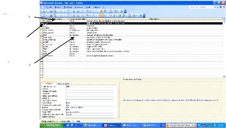
Field name

Primary key

Data type

Figure 3.6: Creation of table in design mode under MS access

· Table assistant mode

Here, access proposes different models of pre-established tables to choose from and create the desired table. The table was then personalized in order for it to suit the conditions required.

· Import table mode

This method has been used for the design of most of the tables that are being presented in this database. The rationale for this was the fact that most of the data concerning the irrigation system has already been stored either as texts or in MS excels spreadsheets. This made it easy for us to import the tables to our database and then define the contents of each field to suit the requirements of our database under the design mode by modifying the specifications of the various fields involved.

· Attach table mode

This method has been used for files that need to remain in their original database such as excel files on which calculations have been done. Hence the link between these files and the attached table in MS access remains and any modification on the file immediately leads to a modification in the attached table. In the calculation of the crop water requirements, the excel spreadsheet on which all the formulas were entered was exported to the database.

3.3.4 Definition of relationships and referential integrity

From the conceptual model of the irrigation system developed we can easily recognize how the different entities of the irrigation system could be related. Most of the relationships retained at the level of the physical model were many-to-one relationships as seen in Figure 3.3. Where we had relationships of the type many to many, we had to breakdown the relationship into two one-to-many relationships. This was done by creating a table between the relationships. For the relationship to be correct, there must be fields in the two tables to link them, even if they have different names, they should contain the same data. Each table has a primary key which is responsible for assuring that there exists some referential integrity between the two tables being linked together. The two tables now become related and this helps easy access and storage of data regarding the irrigation system.

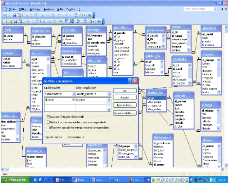
Figure 3.7: Definition of relationships in the physical data model 3.3.5 Creation of data entry and retrieval forms

The procedure for the creation of forms under MS access 2003 has been used for the creation of forms for the irrigation system. This constituted the following procedure:

1) In the Navigation pane, the tables or queries that were needed for the form were selected to use as the form record source.

2) Then we chose Create> More> Forms> Form Wizard. Access displays the first Form Wizard dialog box.

3) For each field we wanted to include in the form, we clicked on the field in the Available Fields list and clicked on the > button. (To select all the fields, we clicked on the >> button.)

4) The next Form Wizard dialog box permitted us to choose the layout of the fields. Four choices are available for this:

· Columnar--the fields are arranged in columns, and only one record is shown at a time.

· Tabular--the fields are arranged in a table, with the field names at the top and the records in rows.

· Datasheet--the fields are arranged in a datasheet layout.

· Justified--the fields are arranged across and down the form with the field names above their respective controls.

5) The next wizard dialog box enabled us to select one of the predefined AutoFormat styles. Click the style you want to use and then click Next.

6) The fourth and last wizard dialog box modifies the name of the form. A suggestion is already in place in the What Title Do You Want for Your Form?? Text box; it is based on the name of the underlying table or query, but the name was entered so that it doesn`t conflict with an existing form.

Figure 3.4 shows a form under construction in MS access environment.

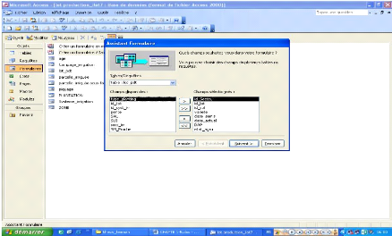
Figure 3.8: Selecting fields to be included in the production plot form under the form assistant mode

3.4 Development of thematic layers for the GIS

The GIS was developed using MapInfo software and AUTOCAD, a computer aided drawing (CAD) software. This type of system gives the possibility of combining methods of simulation of spatial data and the presentation of the results in a graphical manner that will be adapted to the irrigation system of the PHP group. The global architecture of the system will comprise three modules:

· Data entry and update module;

· Water balance module;

· Simulation module;

The thematic layers of the GIS were developed by reviewing the type of data that needed to be entered in the database to meet the specific objectives of the GIS project.

A land use map was developed for the plantation and constituted the main thematic layer for the GIS. The plantation borders, sector, and production plots where been represented. The procedure for creating the land use map with the GPS involved collecting waypoints and extracting the data to a computer. This was done through the following procedure:

1. Creating a folder on the hard drive C\MAPDATA for the data related to the map project. This folder was not stored on the desktop as the files are too large. A permanent folder (not to be moved or renamed) was created, in which the data will remain, as when the maps are saved they reference a pathway to the original data folder.

2. A data cable was connected to the GARMIN 72 GPS unit and to the computer and the GPS unit (simulator mode is fine) was turned on.

3. The DNRGarmin program was then opened. On menu at top, GPS? was been selected, and then Set port? tab to USB

4. Next, the type data we wished to download was clicked, such as waypoint, track or route, then Properties? and then on the tab marked projection?.

5. Once these points have been inserted into the program, we then connect the points to form polygons of the various items we wished to identify in the map.

6. The map was saved on the hard drive and then used later for representation of the various layers which could be shown on the map..

3.5 Calculation of the water requirements in each plot 3.5.1 System requirements

The water requirements of the plots which were been irrigated was calculated by taking into consideration the type of irrigation system concerned as well as the size of the plot and the number of sprinklers on the plot. AUTOCAD 2004 software was used to develop the irrigation map of each plot and the number of sprinklers calculated. Figure 3.5 shows an irrigation map developed with AUTOCAD 2004 software and served as the ground base for calculating the number of sprinklers on a given plot. The number of sprinklers was then entered into the database and the total flow rate calculated automatically by taking the product of the flow rate, the number of sprinklers on the plot and the efficiency of the system involved. Through queries on the database, the total flow rate required for all the plots in production could be calculated.

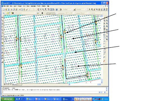
Plot valve

Sprinkler head

N02=Production
plot ID

SF6=Irrigation
plot ID

Figure 3.9: Irrigation map for a production plot developed with AUTOCAD 2004

Through queries on the database, the system requirements of the various plots were been calculated and the results of these printed up in reports or used to create other tables which can be viewed from the forms created. Figure 3.10 shows the environment for the creation of such queries using Microsoft Access 2003 software.

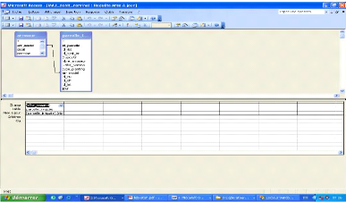
Figure 3.10: Query created in MS access to obtain the water requirements of the system The SQL query created to obtain these values is as follows:

UPDATE arroseur INNER JOIN parcelle_irriguée ON arroseur.arr_model = parcelle_irriguée.arr_model SET parcelle_irriguée.Débit_Nominal = [parcelle_irriguée]. [nbre_arroseur]*[arroseur]. [débit]

3.5.2 Crop water requirements

Crop water requirements were calculated using the water balance equation

S(j+1)^-S(j)= (Peff(j)+I(j))-(ETc(j)-D(j)) (3.1)

S(j+1)-S(j): Variation of available water content

Peff(j) : Effective rainfall

I(j) : Irrigation depth

ETc(j) : Daily crop evapotranspiration

D(j) : Drainage losses

Variation in available water content was computed in the database by taking into consideration the water content of the previous day and that of the following day.

Effective rainfall was computed using equations 2.4 and 2.5 by entering these equations into an excel spreadsheet together with other meteorological data for the different weather station involved. Rainfall after the soil has attained its field capacity and those less than 5 mm/day are being considered non significant to the water balance. These were considered as being lost as runoff or by drainage.

ETc(j) was calculated as a product of the crop coefficient K_c and the reference evapotranspiration ET_p. ET_p values are being entered in the climatic data table in the database as obtained from the records from the various meteorological stations. Corresponding Kc values for the various plots were been used in the database for the different number of days after planting in the plots. The K_c values used in this work are those proposed by Allen et al., 1998. Thus, for each plot ET_c is given by equation 2.7.

Irrigation depth was calculated with respect to the system in place; for microjet sprinkler systems, a factor of 0.9 is used while for undertree systems, a factor of 0.85 is applied and 0.8 for big gun system to take into consideration the efficiency of each system. Thus, the irrigation depth is the product of the quantity of water applied and the correction factor.

On each given date, depending on the events of the previous day (rainfall and evapotranspiration) the quantity of water to be applied was computed for each plot.

Using 20 year climatic data, a probability test for the risk of non satisfaction of crop water requirements was calculated by taking the mean of these requirements within this period for each month. Appendix I shows the procedure used in the calculation of the water requirement as entered in MS excel.

3.6 Evaluation of the Functioning of the Network

One of the five irrigation networks was considered in this study for analysis. Analysis of the network was done by dividing the network into various branches and taking into consideration the number of hydrants which are opened upstream during irrigation. Hydraulic calculations were done based on the formulas proposed by Zoungrana (2002) while heads losses were calculated using the Hazem-William equation. Microsoft Excel software was used for the hydraulic analysis.

3.6.1 Calculation of flow rates

If (en m³/h) is the nominal flow rate of one big gun, n the number of opened big guns upstream and (m³/h) the flow rate from the extremity of the downstream branch,

the flow rate entering the upstream branch, (m³/h) is given by the formula:

(3.1)

The flow rate leaving the downstream branch is calculated by respecting the loop rule of networks which is derived from the principle of conservation of matter as:

? Flow entering = flow leaving (3.2)

Given that the network functions both in the transport and distribution of water, the hydrants have almost equal flow rates. The flow rate which results in the same head loss

4 ? Q

? otherwise known as the fictitious or simulated flow rate,

? ?

? 10 ? 3600

D ? (m³/h), was calculated by the

formula presented by Zoungrana (2002):

(3.3)

3.6.2 Calculation of flow velocity and head losses.

Given that the flow rate in the conduits follows steady state conditions for the same pipe diameters (i.e. the velocity in the fluid is the same in both magnitude and direction at a given instant and in at every point in the fluid), the flow velocity was calculated by applying the formula:

(3.4)

Where:

= Flow velocity (m/s)

= Flow rate considered (m³/h)

= internal diameter of the conduit (mm)

Also the velocity of flow in water supply conduits is always less than or equal to 1.5m/s so knowing the diameter of the conduits, the velocity of flow could be generated.

, but

Head losses were being calculated using the Hazem-William equation

(3.5)

Where,

Linear head losses (m)

L= length of given branch (m)

Q= fictitious flow rate (lps)

C=150 for plastic pipes and 120 for steel pipes D= internal diameter of pipe (mm)

Singular head losses due to T`s, bends, valves and elbows which are difficult to calculate are estimated to be 10%

(3.6)

Total Head Losses, J, in a given branch is the sum of the linear and singular head

losses

(3.7)

The ratio of this head loss on the length of a given branch gives us the unit head losses given by:

(3.8)

Where,

j = unit head loss (m/m)

L = length of branch (m)

J = head loss in a given branch (m)

3.6.3 Determination of available and required pressures

At the level of each hydrant, the available pressures and the required pressures were calculated as follows:

(3.9)

Where,

available pressure upstream (m)

available pressure downstream (m)

upstream piezometric elevation (m)

downstream piezometric elevation (m) = head loss in a given branch (m)

The required pressure downstream equals zero, if the number of big guns at the

??

downstream hydrant equals zero or equal to the required pressure upstream if the number of big guns at the downstream hydrant is different from zero.

The pressures available upstream used in our calculations are those of the technical slip of the principal conduits of PHP, version 2 of 16/02/01.

These calculations were done taking into consideration the canon or the plot with the worst case (i.e. the furthest big gun on relatively flat ground or the most elevated or both). The other systems such as the microjet and undertree systems were been converted into the equivalent number of big guns. This is because this system sets the ground base for the conversion to other systems.

For undertree irrigation systems, the pressure required at the entry of a lateral is given by the formula proposed by Azenkot (1999), considering that the terrain is relatively flat.

hu = hs + 3/4F + r (3.10)

Where,

hu = pressure required at the entry of the lateral (m) hs = nominal pressure of sprinkler (m)

F = correction factor

= linear head loss in the lateral (m)

r = height above the ground of the sprinkler (m)

The pressure required at the center of the primary conduit is calculated in the same way as that of the laterals and is given by:

hr = hu +3/4(Fr ) (3.11)

Where,

hr = required pressure at the centre of the lateral (m) Fr = correction coefficient of the lateral

= head losses in the lateral (m)

? P avn ? Z av

The pressure available at the entry of the secondary conduit or hydrant is given by equation 3.2:

= hr + + Zp - z (3.12)

Where,

= pressure required at the hydrant (m)

= head losses in the secondary conduit (m)

Zp = geometric elevation of the hydrant

z = geometric elevation of the plot with the worst case (m)

For irrigation plots totally covered by big guns, the required pressure is calculated as above, the only exception being that the correction factor is considered to be unity (1).

3.6.4 Calculation of piezometric elevations

The piezometric elevations are calculated based on the following formula proposed by Zoungrana, 2002

. piezometric elevation required downstream

(3.13)

Where,

piezometric elevation required downstream (m)

required pressure downstream (m) downstream elevation (m)

. piezometric elevation required upstream

(3.14)

Where,

required piezometric elevation upstream (m)

required pressure downstream (m) upstream elevation (m)

. available piezometric elevation upstream

(3.15)

Where,

available piezometric elevation upstream (m)

required piezometric elevation downstream (m)

= head losses in the given branch (m) . piezometric elevation retained upstream

max ( , ) (3.16)

Where,

piezometric elevation retained (m)

3.7 Spatial Representation of some Aspects on the Irrigation System

Spatial representation of some aspects on the irrigation system was done under MapInfo and AutoCAD software. Multiple queries on the MS access data base was carried out to be able to obtain the data that needed to be represented spatially. An ODBC connection between the database and the MapInfo software was created to be able to represent these aspects of the irrigation system. Queries led to the creation of tables in database formats (dbf) which helped to link them to the land use map of the plantation. This

is because tables are linked by the plot ID which is a common denominator to both tables. For example, to represent spatially the plots which have the microjet irrigation system, a query was created on the plot table which has one of its columns being the plot ID same as that for the map table.

CHAPTER IV
RESULTS AND DISCUSSIONS

4.1 Database for the Irrigation System

The process of development of a database for the system led to the realization of a model for the data concerning the irrigation system.

4.1.1 Physical model

The physical model of data shows how the various tables of the database have been linked based on the relationships that exist between the various entities in the tables (Figure 4.1). It could be seen from this model that a zone for example, will comprise several plantations, a plantation will comprise several sectors etc. These relationships thus developed govern the mode of querying data for the irrigation system. Based on the information that is required at any point in time, the irrigation manager could query tables that are linked to the information that is required for the system.

The relationship between the different tables is presented as it was lastly defined and thus, is not standard. The fields of the different tables are equally not final and modifications could be envisaged after a trial period of the GIS database. This method of organizing data will greatly improve management of the irrigation system as the irrigation manager could simulate any field situation and obtain the information that is required.

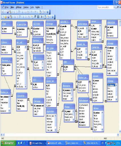
Figure 4.1: Presentation of the physical model of data as developed in MS Access

4.1.2 Creation of forms

Ten forms for the irrigation system were created and the layout of one of these forms is presented in Figure 4.3.

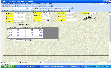
Figure 4.2: Form for data entry and retrieval for the production plot

Forms bring a number of advantages to the data entry table:

· Because the form shows only one record at a time, the irrigation manager can almost always see all the table fields at once, contrary, to datasheets were it is only possible to see only four or five columns at a time.

· Controls such as drop-down lists reduce the possibility of data entry errors by giving the users a limited set of choices for a field.

· Access will give irrigation managers a number of customization options. These features let them create Access forms that look exactly like paper forms, and they can add graphics and other objects to make the forms more interesting.

· The irrigation manager will not be distracted by other data in the table, and thus give full attention to the task at hand.

Specifically to the irrigation database, the forms give users the possibility to enter and retrieve information without having to open the tables involved. One could for example want to know the plots that are irrigated in a particular production plot, to replace a plot that is now under fallow, to enter a new irrigation plot etc. This will be easily done with the use of forms. Some of the forms created included that of the irrigation plots, production plots, the age of the plantation and a total of 10 forms were created to enhance data entry and retrieval.

4.2 Thematic layers for the GIS

Tables 4.1, 4.2 and 4.3 show the various data that have been entered into the database to constitute the thematic layers for the GIS. The various layers have different uses in the database such as the geographical location of the various soil types, equipments on the irrigation system, creation of water requirement maps, digital elevation maps, and determination of ET_c etc.

Table 4.1: Thematic layers for simulation of the functioning of the network

Thematic layer of GIS	Mode of representation	Principal objectives		Data source	Hydrants
Vector (polyline)	Visualize in a georeferenced space the various hydrants	Irrigation Service		Irrigation
	Visualize in a georeferenced			Network
Vector (polyline)	space the various equipments of the water supply system	Irrigation Service
	Visualize access for			Road network
Vector	maintenance works on the	DST
(polyline))	Irrigation system			Contour lines
Vector	Create a DEM to determine the altitude at each point in
(polyline)	the plantation	DST		Equipments on
Vector	Visualize in a georeferenced	Irrigation		Irrigation System
(polyline)	space all equipments on the primary, secondary and tertiary network	Service

shp=shape file, dbf=database format, DEM=Digital elevation model, GN=Grand Nain cultivar, W=William cultivar

Table 4.2: Thematic layers needed for water balance calculations

Thematic layer of the GIS	Mode of representation	Principal objective(s)		Data source	Zonal boundaries of
				PHP Sud
Vector (polygon)	Create a DEM	.shp File
		Associated to a
	Geographically locate all objects present in this limit	.dbf File		Boundaries php1-2-3-4-5
Vector (polygon)	Create a DEM	.shp File
		Associated to a
		.dbf File		Sector boundaries
Vector (polygon)	Create a DEM	.shp File
		Associated to a
		.dbf File		Production plot boundaries
Vector (polygon)	Create a DEM	.shp File
		Associated to a
		.dbf File		Boundary of spatial occupation, GN cultivar
Vector (polygon)	Create a DEM	.shp File
		Associated to a
		.dbf File		Boundary of spatial occupation, W cultivar
Vector (polygon))	Create a DEM	.shp File
		Associated to a
		.dbf File		Soil types
Vector (polygon)	Create a DEM et	Soil map from the
	Visualise in a	Direction
	Georeferenced space the	Agrononiques? et de la Recherche
	Various soil types in the plantation	(DAR)		Meteorological
				Stations
Vector (polygon)	Visualise in a
	Georeferenced space the various stations	DAR
	Create ETP, climatic data, and water requirement maps			Rainguages
Vector (polygon)	Visualise in a
	Georeferenced space the location of the rainguages	DAR		Crop developmental
	Create a DEM of the production plots	Direction de		stages
Vector (polygon	concerned	Production (DP)

Table 4.3: Thematic layers for non-descriptive data

Non Spatial Principal Data

data Characteristics Manipulation Simulation objective(s) source

Crop Variety

Developmental stage Modelling

Crop coefficient Crop water Irrigation Topological DP

Height above the ground Requirements scheduling Description

Max rooting depth Statistical analysis

Min rooting depth Simulation
Depletion level

Yield factor

Planting date

Soil Field capacity

Wilting point Determination of

TAWC the soil type

RAW Available Water Irrigation Calculate soil DAR

Infiltration rate Content scheduling moisture deficit

Calculate soil

% Clay moisture

% Sand Content

% Silt

Maximum rooting depth

Climate Temperature Rainfall ETp Irrigation Relative humidity ETc scheduling

Calculate crop water requirements and water DAR

Wind speed loss by the plants

Sunshine hours

Effective Precipitation

Production Surface area Calculate quantity

Plot Agronomic state of water consumed

Crop variety Quantity of Irrigation Modeling DP

Planting date Water required scheduling Spatial arrangement on the plot Soil type

Water-plant- atmosphere Determination of the terms of the water balance equation

Water deficit Calculate irrigation

Slope Efficiency
Irrigation system

4.3 Water requirements in each plot 4.3.1 System requirements

The system water requirements vary with respect to the system in place. From the database, the quantity of water that was needed by each plot was obtained. The number of sprinkler heads which function simultaneously and the efficiency of the system concerned were considered in these calculations. Figure 4.3 shows a report of a query to calculate the system requirement using MS Access 2003.

The various systems found in the PHP group and their characteristics are: Big gun (canon) system

Rain bird big guns: 60 m³/h at 5 bars

Rainfall depth: 10 mm/h

Microjet system

Rondo type: 300 l/h at 1.5 bars

Rainfall depth: 3 mm/h

Undertree system

Rain bird type: 620 l/h at 3.0 bars

Rainfall depth: 4.78 mm/h

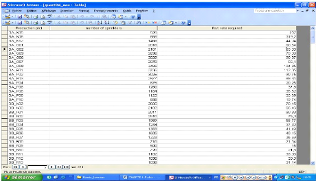
Figure 4.3: System water requirement as calculated in MS access

4.3.2 Crop water requirements

Climatic data for a period of 20 years (1989-2008) from meteorological stations in the plantation were used in this study. These stations provide rainfall and pan evaporation data.

The average annual rainfall varies from 2400 mm to 3200 mm and distributed as thus in the plantation, with Mantem being the highest in elevation and Bonanadam the lowest in altitude:

Mantem : 3200 mm/yr

Loum : 3200 mm/yr

PHP-haut : 2800 mm/yr

Dia-Dia, Bonandam : 2600 mm/yr

Sir, Mpoula : 2500 mm/yr

Four : 2400 mm/yr

There seems to exist a relationship between altitude and rainfall and enables us to distinguish the high altitude plantations (Mantem and Loum), low altitude plantations (DiaDia, Bonandam, Mpoula, Sir and Four) and intermediate altitude plantations (PHP-haut). The evapotranspiration was calculated in the database by applying a pan coefficient, Kp of 1.1 as indicated by Allen et al. (1998) and the crop coefficient as given by the database.

The RAW was found to vary by a factor of 10 with respect to the type of soil and by a factor of 4 with respect to root depth. The RAW was considered to be 10 mm for every 10 cm of root depth.

A probability study for the risk of non satisfaction of the crop water requirements was done on the 20 years climatic data available. All the rainfall data was assumed to be effective because of the following reasons:

· Rainfall in the dry season are the most susceptible to modify the terms of the water balance equation. We thus considered that during this period due to the physical properties of the soil (high water retention, high hydraulic conductivity), the quantity of water loss as run-off and drainage is negligible.

· Rainfall data obtain were already cumulated for each month and it was therefore difficult to distinguish rainfall that are less than 5 mm/day as proposed by Smith et al. (1998).

· Most of the soils of the group are andosols and hence have a high capillarity. This upward movement of water is thus considered to compensate for the non effective rainfall.

Table 4.4 gives the probability of satisfaction of irrigation requirements for a total of 20 years so as to better schedule irrigation with the use of the database knowing the risks that could arise I these water requirements are not fully satisfied. The table shows a summary of the average monthly water requirements for banana in the area.

Table 4.4: Probability of satisfaction of crop water requirements (requirements in mm)

	Jan	Feb	Mar	Apr	May	Jun	Jul	Aug	Sep	Oct	Nov		Dec	1 yr/2
>102	>69	0	0	0	0	0	0	0	0	>31	>98		1 yr/5
>137	>127	>50	0	0	0	0	0	0	0	>82	>127		1 yr/10
>144	>139	>65	=0	=0	=0	0	0	0	0	>123	>139		1 yr/20
172	138	124	64	34	36	0	0	0	9	133	149

If we consider a probability of satisfaction of crop water requirements 1 yr out of 5, then we need to apply a total of 137 mm of water per month, an average of 32 mm/week.

If this risk of satisfaction is considered to be 1 yr/10, the quantity of water to be brought in through irrigation is 144 mm per month, giving an average of 33.5 mm/week.

Taking a risk factor of 1:20, that is, satisfying the crop water needs 1 out of 20 years, the water required by the crops will be 172 mm per month giving an average requirement of 40.2 mm/week for an average root depth of 50 cm.

With respect to the irrigation systems this water requirement could further be adjusted by applying the efficiency of the system, _Keff. Table 4.5 thus shows the weekly dose of water to be applied taking into consideration the various satisfaction probabilities and the irrigation system concerned.

Table 4.5: Irrigation dose (mm) for two irrigation systems

Probabilty of non satisfaction Undertree Microjet

of irrigation water Keff =0.8 Keff =0.9

requirements

1 year/2	30		26	1 year/5
40	35		1 year/10
42	37		0 risk
50	45

This water requirement is been fractioned and applied three times in a week for soils with light textures as shown in the irrigation calendar in Appendix II. Thus for an application of 40 mm a week, the application could be 13.3 mm in 3 days.

When this water requirement is calculated, depending on the events of the previous day, the value is adjusted in the database. If for example, we simulate a situation where the effective rainfall is say 10 mm and that ET_c is 4 mm then for a 21.3 mm crop demand, we would apply only 7.7 mm after a reduction of _Peff and ET_c. This shows that 7.7 mm of water could be saved. This could lead to reduction in the pumping time and cost of operation and increase in marginal profits.

4.4 Simulation of the Functioning of the Network

Analysis of the network shows that the total length of the networks is 7 056 m and that the total amount of water that could be transported in the whole network is 5 313 m³/h. With a simulated manometric height of 240 m, the service pressure is 24 bars, while the total head losses in the network is 19.7 m. This gives a loss in pressure of approximately 2 bars. The flow velocity in the various branches vary from 0.8 m/s - 1.1 m/s and are in accordance with the norm ( ) for flow in closed conduits described by Zoungrana, (2002).

The different parameters calculated and the hydraulic characteristics of the network are presented in Appendix III. The flow velocities, the roughness coefficient, the deviation in pressure at the level of the hydrants, the cumulated head losses and the total manometric height are the principal characteristics emphasized on.

The manometric height of the pumping station is obtained as the difference between the retained piezometric elevations upstream and the geometric elevation of the pumping station. Where ever the manometric height considered is less than that which is calculated, the network is said to be mal functional. Where total head losses in the pipe are less than 10% of the service pressure at the pumping station (HMT), and where there exist insufficient pressures in a hydrant, a suppressor will be needed in order to increase the available pressure at the hydrant. Where head losses are greater than 10% of service pressure at the pumping station and that the pressures at the hydrants are sufficient or not, these pressures need to be reduced.

4.5 Spatial Representation of some Queries on the Irrigation System

The database created helps the irrigation manager to inquire information related to irrigation project in GIS environment. Either Permanent data or yearly changing data can be inquired in the database. Some examples of created queries are as follows:

- Parcel irrigated during a given production year

- Crop pattern under selected channel

- Geographical position of plot valves

- Type of irrigation systems in various plots

- Crop pattern under selected parcel

4.5.1 Spatial representation of crop coefficients

The sensibility of crops to water stress is represented spatially as show in Figure 4.4 by considering the crop coefficients for the various production plots and the soil types involved. This helps managers in the localization of plots with critical conditions and hence enhances decision making. Thus, in the case of water shortage and only few plots could be irrigated, the plots with a critical response to stress will be satisfied first. This done through a query of the database and the result presented in the GIS. Figure 4.4 therefore illustrates that in order to take a management decision for irrigation, the plots shaded in green on the map have to be irrigated before those in orange. These plots either have plants with a higher vulnerability to water stress or are found on plots whose soils are of light texture and thus need frequent irrigations.

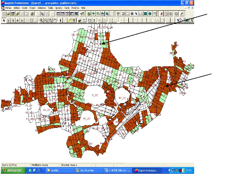
Plots with a higher sensibility to water

Lower sensibility

Figure 4.4: Sensibility of various plots to water stress with respect to K_c

4.5.2 Spatial representation of some plot valves

For interventions on the plots, prompt actions could be taken if the exact valves that need to be opened or closed are being represented graphically as shown. When water becomes a limiting factor, particular plots which to be privileged could thus be quickly identified and satisfied. This is obtained through queries on the database and the results represented spatially on map as shown in Figure 4.5. In case of a repair intervention on a given plot, the exact valve to be closed is easily recognized geographically from the map. Another utility of such a map could be in the regulation of pressure on a given plot during periods of water shortages, by closing the valves which have plants which are less sensitive to water stress and opening those of plots with a high sensitivity to water stress.

Plot valve Secondary pipe

Figure 4.5: Plot valves for two irrigation plots

4.5.3 Theissen polygon for rainfall heights on the plantation

Rainfall heights entered in the database from the different meteorological stations are being interpolated to get the rainfall in plantations with no rain gauges using the MapInfo GIS software. The distribution of rainfall within the different plots in the plantation could be obtained spatially and integrated into maps to get the rainfall depths for other portions of the plantation with no rain gauges. Figure 4.5 shows the distribution of rainfall depths in the plantation after a rainfall in the plantation. The irrigation manager uses this information to adjust the water requirements of each plot in the water balance equation by knowing the amount of rainfall that is received each plot. This is to minimize energy used in pumping of water and hence to maximize profits from the sale of bananas.

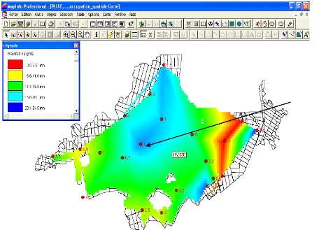
Position of rain guage

Figure 4.6: Repartition of rainfall depths in the plantation

CHAPTER V: CONCLUSIONS AND RECOMMENDATIONS 5.1 Conclusions

Based on the methodology used and the analysis of results:

· A total of 17 tables for the various aspects pertaining to irrigation management have been developed for the database. The main aspects such as the crop coefficients of the various production plots, the irrigation systems involved etc. These tables developed help in enhancing data entry and retrieval through the use of forms and queries.

· Thematic layers for the GIS such as the soil types, the boundary/limit of the various plots have been determined by the use of a map of the plantation developed with the use of a GPS. This land use map constituted the main thematic layer for the GIS.

· The crop water requirements were calculated to be 40 mm for an average rooting depth of 50 cm for the irrigation of banana in the area. The probability of satisfaction reveals that, this depth of water will satisfy crop water requirements 1 year out of 20. The water requirement will be adjusted in the database depending on the ET_c and _Peff of the previous day or week.

· Analysis of the existing network revealed that, the system in place is functioning properly considering the pressures and flow rate required. The flow velocities (0.8=V= 1.1 m/s) in the different branches of the network show that they are satisfactory. This shows that if there exist deficiencies in the system this could be only due to scheduling options as earlier stated by Sisodia, (1992).

· Maps have been developed for plot valves, position of rain gauges in the plantation, the type of irrigation system involved, the sensibility of the various plots to water stress and other aspects related to the irrigation system and which are necessary for the calculation of the water requirements have been represented spatially to help irrigation managers in the aspects of irrigation scheduling. Maps for any event on the plantation could thus be printed out and given to the technicians for execution of particular tasks on the irrigation system.

The irrigation network has undergone some form of evaluation and monitoring. For instance, monitoring of the flow rates in the main irrigation canals has been carried out. If

this type of information is available in a GIS format, evaluation and monitoring can be made easier, timely and cost-effective.

5.2 Recommendations

5.2.1 Improvement of the system

· Organization of data for the system should be a main priority for the Group. This will help to have more realistic values for use in the GIS.

· Rain gauges should be redistributed in the plantation in order to get a more coherent repartition for rainfall data which forms one of the basic entities of the water balance equation.

· An internal network between computers should be created with the various sources (DST, DAR, DP) such that, information should be readily accessible. This will decrease the time needed for obtaining information for the installation of a particular irrigation system on any portion of the plantation and the monitoring of its water requirements

· Tensiometers need to be installed in the production plots to compute the adequacy between the water supplied to the banana plants and that which is consumed.

5.2.2 Further research

· A user interface between the MS access database and the Mapinfo GIS software
needs to be created to give a more user friendly and convivial work environment.

· The database needs to be equally linked to decision models such as hydraulic and agro-economic models to help managers in the understanding of which option to use when confronted with several decision options.

REFERENCES

Adam, H., Beaudequin, D., 1997. Matériels et Systèmes d`Irrigation et Drainage. In Rôle et Objet de ISO/T3/SC18. Proceedings of the ICID-ISO Workshop on the Standardization of Irrigation Equipment, 11 September 1995. FAO Water Reports N° 8, FAO, Rome, Italy, 76 pp.

Allen, R.G., Pereira, L.S., Raes, D., Smith, M., 1998. Crop Evapotranspiration: Guidelines for Computing Crop Water Requirements. FAO Irrigation and Drainage Report, Rome, 300 pp.

Alvanker, R., Mousavizadeh, M. H., Nazari, M., 2000. Application of GIS in Water Resources Studies. Fourth Conference of Iranian Commission on Large Dams. January 5-10, 2000, Tehran, Iran. 48 pp.

Amor, V. M., DAS GUPSTAL, A., LOOF, R., 2002. Application of GIS and Crop Growth Models in Estimating Water Productivity. Journal of Agricultural Water Management 54, pp. 205 -225.

Anonymous, 1998. Estimation des Chiffres Mondiaux de Production et Commercialisation de Banane. FRUITROP 51, pp. 9-10.

Anonymous, 2003. Dossier Filière Banane. In Cameroon Tribune, N° 7841/4130, 31pp.

Aquastat, 2009. FAO Information System on Water and Agriculture, FAO, Rome. Obtainable from www.aquastat.org

Atangana, J. B., 2003. Présentation et Etude Comparée de quelques Dispositifs de Plantation du Bananier (Musa acuminata Colla) : Cas des Plantations Industrielles de la SBM-Loum. Unpublished « Ingénieur Agronome » thesis, Department of Crop Science, University of Dschang, Dschang, Cameroon. 58 pp.

Azenkot, P. M., 1999. Irrigation, Guide Pratique. 2e Edition. CEMAGREF, Antony; edition France Agricole, Paris. 245 pp

Beernaert, F., Bitondo, D., 1993. Land Evaluation Manual. Department of soil Sciences, University of Dschang, Dschang, Cameroon, 212 pp.

Boa, A. P., 2005. Optimisation des Pertes de Charges dans le Réseau d`Irrigation des Plantations du Group PHP-SBM de Njombé. Unpublished « Ingénieur Agronome » thesis, Department of Agric. Engineering, University of Dschang, Dschang, Cameroon. 101 pp.

Borg, A. H., Grimes, D. W., 1986. Depth Development of Roots with Time: An Empirical description. Transactions of the American Society of Agricultural Engineers 29 (1): pp. 194-197.

Chang, K., 2007. Introduction to Geographic Information System, 4th Edition. McGraw Hill, London. 231 pp.

Codd, E. F., 1970. A Relational Model of Data for Large Shared Data Banks. Communications of the ACM 13 (6): pp. 377-387.

Collazzi, P. D., Sscheider, A. D., Howell, T. A., Evett, S. R., 2003. Comparison of SDI, LEPA, and Spray Efficiency for Grain Sorghum. ASAE Annual International Meeting. July 27-30, 2003, Las Vegas, Nevada. American Society of Agricultural Engineers. Central Plains Irrigation Association, Colby, Kansas. pp. 54-69.

Cremona, V.M., Witich, K.P., Sourell, H., 2000. The use of the crop water stress index in humid climates. Zeitschrift für Bewässerungswirtschaft 34. Zurich, Germany. pp. 175-192.

Daneshkar, A., P., Shokoohi, A., Hassandvand, A. M., Saghafian. B., 2000. Application of GIS and Geostatistics in Groundwater modelling. GIS Conference in Iran, February 24-29, 2000, Tehran, Iran. 43 pp.

Dayyani, S., Mouhammadi, K., Mousavizadeh, M. H., 2003. Irrigation and Drainage System Management using GIS. Presentation at the CSAE/SCGR meeting, July 6-9, 2003. Montréal, Québec. 37 pp.

Defo P. M., Marie P., 1998. Proposition des techniques de préparation des sols pour
planting, Direction des Services Techniques PHP, Njombe, Cameroun. 10pp.

Delvaux, B., 1995. Soils. In Gowen, S. R. (ed.), Bananas and Plantains. Chapman and Hall, London. pp. 230-257.

Doorenbos, J., Kasam, A. H., Bentvelsen, C. L. M., Branscheid, V., Plusje, J. M. G. A., Smith, M., Uittenbogaard, G.O., Van Der Waal, H. K., 1986. Yield Response to Water. FAO irrigation and drainage paper 33, Rome. 234 pp.

Encarta, 2008. Microsoft Encarta and student program manager one Microsoft way. Microsoft Corporation. Redmond, USA.

ESRI, 1996. ArcView GIS: The Geographic Information System for everyone. Environmental Systems Research Institute, ESRI, Inc., Redlands, USA. 67 pp.

Evans, R., Sneed, R. E., Cassel, D. K., 1996. Irrigation Scheduling to Improve Water and Energy Use Efficiencies. North Carolina Cooperative Extension Service, AG 452-4. 134 pp.

Ewane, E. H., 2008. Evaluation of the Undertree Irrigation System of the CDC Ekona Banana Plantation (EBP) Mussaka. Unpublished Ingénieur Agronome? thesis, Department of Agric. Engineering, University of Dschang, Dschang, Cameroon. 67 pp.

Fonsah, E. G., and Chidebelu A. S. 1995. Economics of Banana Production and Marketing in the Tropics: A Case Study of Cameroon. Minerva Press London. 230 pp.

Fonteh, F. M., Assoumou, E. E., 1996. Irrigation and Drainage: Distance Education Course
Notes, DE 011GR. University of Dschang, Dschang, Cameroon. 172 pp.

Google Earth, 2009. Google earth Version 5.0.11337.168 (beta). Data: US Navy, Europa Technologies, Tele Atlas, Map Link. Google Corporation. USA.

Hanks, R. J., Ashccroft G. L., 1980. Soil Water and Temperature Application. In Bommer. D. F. R., Sabey. B. R., Thomas. G. W., Vaadia Y., (Eds.). Applied Soil Physics. Springer. New York. 189 pp.

Heywood, I., Cornelius., Carver, S., 2006. An Introduction to Geographical Information Systems, 3^rd Edition. Prentice Hall, London. pp. 195.

Hoogenboom, G., Jones, J. W., Boote, K. J., 1991. A Decision Support System for Prediction of Crop Yield, Evapotranspiration, and Irrigation management. In: Ritter, W. F. (Ed.) Irrigation and Drainage (Proc., 1991 Nat. Conf,), American Society of Agricultural Engineers, New York: pp. 198-204.

Howell, T. A., 2003. Water Loss Comparisons of Sprinkler Packages. Central Plains Irrigation Short Course and Exposition. February 4-5, 2003, Colby, Kansas. 98pp.

James, D. W., Hanks, R. J., Jurinak, J. J. 1982: Modern irrigated soils. A Willey - Interscience Publication. John Wiley & Sons, New York. 345 pp.

Jensen, M. E., 1981. Irrigation Scheduling for Water and Energy Conservation in the 80s: In Fereres, E. 1996, Irrigation scheduling and its impact on the 21s century. Proceedings of the international conference of the American Society of Agricultural Engineers. San Antonio, Texas, USA, November 3 - 6.

Kopec, A. R., Langley, M. N., Bos, M. G., 1984. Major Variables which Influence Effective Precipitation. ICID Bulletin 33 (2): 68 - 84. In: Rojas, R., Rolda'n, J. (eds.). Evapotranspiration mapping and irrigation scheduling for olive trees. Evapotranspiration and irrigation scheduling. Proceedings of the international conference of the American Society of Agricultural Engineers. San Antonio, Texas, USA, November 3-6.

Kramer, P.J. (1983). Water Relation of Plants. Academic Press Inc, New-York, USA. 489 pp.

Lane, I. E., 1955. Genera and Generic Relationships in Musaceae. Mitt. Bot. Staatssman 45, Muchen, Germany, pp. 141-131.

Lassoudiere, A., 1979. Croissance et Développement du Bananier Poyo en Cote d`Ivoire. These, Université Nationale de Cote d`Ivoire, Abidjan, Cote d`Ivoire. 312 pp.

Lemeilleur, S., Temple, L., Kwa, M., 2003. Identification of Banana Production Systems in Urban and Peri-urban Agriculture in Yaoundé. The International Journal on Bananas and Plantains (INFOMUSA), 12:1, pp. 13-16.

Marty, P., 1983. Fiches Techniques d`Agriculture Spéciale. Le Bananier, Série 2, Ministère de la coopération, Paris, pp. 3-15.

Menenti, M., AzzaliI, S., D`Urso, G., 1995. Management of Irrigation Schemes in Arid Countries. In: Vidal, A. (Ed.) Use of Remote Sensing Techniques in Irrigation and Drainage. FAO, Rome, pp. 1-98.

Merriam, J., Keller, J., 1975. Farm Irrigation Evaluation: A Guide for Management. Utah University Press, Utah, USA. 156 pp.

Molden, D. J., Saktivadivel, R., Christopher, J., Perry, De Fraiture, C., Kloezen, W. H., 1998. Indicators for Comparing Performance of Irrigated Agricultural Systems. Research Report N° 20, International Water Management Institute, Colombo, Sri Lanka. 35 pp.

Moon, D., Van Der Gulik, W., 1996. Irrigation scheduling using GIS. In Evapotranspiration and Irrigation Scheduling. Proceedings of the International Conference of the American Society of Agricultural Engineers. San Antonio, Texas, USA, November 3-6. pp. 644-649.

Njila, R. C., 1999. Evaluation du Systéme d`irrigation par aspersion à la Tiko banana plantation. MSc. thesis, Faculty of Agronomy and Agricultural Sciences, University of Dschang. 97 pp.

Pedro, A., Cora, D., Pascal, L., Paul, P., 2003. The World Banana Economy 1985-2002. FAO, Rome, Italy. 55 pp.

Plauborg, F., Andersen, M. N., Heidmann, T., Olesen, J. E, 1996: MARKVAND: A Decision support system for irrigation scheduling. Evapotranspiration and irrigation scheduling. Proceedings of the international conference of the American society of agricultural engineers. San Antonio. Texas. USA. November 3-6. pp. 527-535.

Ray, S. S., Dadhwal V. K., 2001. Estimation of Crop Evapotranspiration of Irrigation Command Area Using Remote Sensing and GIS. Journal of Agricultural Water Management, 49: pp. 230-249.

Rieul, L., Delacourt, A., Revol, P., Ruelle, P., 1992. Prévention de la Pollution des Eaux par Ruissellement et par Percolation hors d`atteinte du système Racinaire dans le cas des Cultures irriguées. Proposition pour le code de la bonne pratique agricole, Annexe 2, Paragraphe 10. CORPEN Editeur, Paris. 192 pp.

Riopel, J. L., Steeves, T. A., 1964. Studies on Roots of Musa acuminata cv. =Gros Nain`. Ann. Bot. Lond., NS, pp. 90-115.

Robinson, J. C., 1981. Water Requirements of Bananas. Agriculture and Fisheries Department, Pretoria, South Africa. 57 pp.

Robinson, J. C., 1987. Root Growth Characteristics in Banana. ITSC Information Bulletin, N° 183, Wallingford, UK, pp. 7-9.

Robinson, J. C., Alberts, A. J., 1987. The Influence of Under Tree Canopy Sprinkler and Drip Irrigation Systems on Growth and Yield of Bananas (Cultivar Williams) in the Sub Tropics. Sci. Hort. 32. pp. 49-66.

Robinson, J. C., Anderson, T., 1991. The Influence of Temperature on Dry Matter Assimilation and Distribution in Young Banana Plants. Newsletter of the International Group on Horticultural Physiology of Banana, 14. pp. 36-37.

Robinson, J. C., De Villier, E. A., 2007. The Cultivation of Bananas. ARC-Institute of Tropical and Sub Tropical Crops, Du Roi Laboratory, Pingwe Print, Nelspruit, South Afica. 258 pp.

Rojas, R., Rolda`n, J. 1996: Evapotranspiration mapping and irrigation scheduling for olive trees. Evapotranspiration and irrigation scheduling. Proceedings of the international conference. American society of agricultural engineers. San Antonio, Texas, USA, November 3-6. 278 pp.

Sarangi, A., Rao, N. H., Brownee, S. M., Singh. S. A., 2001. Use of Geographic Information System Tool in Watershed Hydrology and Irrigation Water Management. Retrieved 24^th April 2009 from http://www.GISdevelopment.net .

Schwab, G. O., Fangmeier, D. D., Elloit, W. J., Frevert, R.K., 1993. Soil and Water Conservation Engineering, 4^th ed. John Wiley & Sons, Inc. New York. 234 pp.

Sisodia, J. S., 1992. Performance Monitoring Study of the Warabandi Irrigation Management System of in the Chambal Area. Indian Journal of Agricultural Economics, 47:4. Calcutta, India, pp. 23-45.

Smith, M., Pereira, L.S., Berengena, J., Her, B., Goussard, J., Ragab, J., Tollefson, L., Van, H., 1996. Irrigation Scheduling: From Theory to Practice, FAO International Commission on Irrigation and Drainage, Rome. 384 pp.

Stover, R. H., 1979. Pseudostem Growth, Leaf Production and Flower Initiation in the Grand Nain Banana. Trop. Agric. Res. Services (SIATSA), La Lima, Honduras. 118 pp.

Stover, R. H., Simmonds, N. W., 1987. Bananas (3^rd Ed.). John Wiley & Sons Inc, New York, USA. 468 pp.

Summerville, W. A. T., 1939. Root Distribution of Banana. Quensl. Agric. J., pp. 70-96.

Swennen, R., Vuylteke, D., 2001. Le Bananier. In Plantes à Fruits. Agriculture en Afrique, pp. 611-637.

Taylor, B. B., 2005. Comprehensive Water Resource Management through Geographic Information Systems. Proceedings of the 2005 Georgia Water Resources Conference, held April 25-27, 2005, at The University of Georgia, Georgia, Athens. 123 pp.

Tchiadje T. N., 1995. Optimisation de l`exploitation des réseaux d`irrigation de la SPNP. Rapport de stage d`insertion professionnelle. INADER, Université de Dschang, Cameroun.

Thome, P. G., 2007. Etude Comparée de Deux Dispositifs de Système Micro Jet dans une Bananeraie Plantée en Ligne Jumelées au Group PHP-SBM. Unpublished « Ingénieur Agronome » thesis, Department of Agric. Engineering, University of Dschang, Dschang, Cameroon. 78 pp.

Tiercelin, J. R., 1997. L`Irrigation des Parcs et Jardins. Lavoisier Technique de Documentation, Paris, pp. 345-415.

Tron, G., Isberie, C., Chol, P., 2000. La Tensiométrie pour Piloter les Irrigations: Une Gestion Raisonée de la Ressource en Eau. Educagri editions, Dijon Cedex, France. 247 pp.

Turner, D. W., Lahav, E., 1983. The Growth of Banana Plants in Relation to Temperature. Australian Journal of Plant Physiology, 10. pp. 43-53.

Valmayor, R. V., 1991. Banana Classification and Commercial Cultivars in Southeast Asia.
PCARRD Information Bulletin N° 24, Los Banos, Philippines. pp. 15-20.

Van De Pol M. J., Nsoyuni L. A., Minnemeyer S., Ngoufo R., 2005. Atlas Forestier Interactif du Cameroun. MINEF, World Resources Institute, Global Forest Watch. Washington. 244 pp.

Van Laere, P. E., 2003. Memento de l`Irrigation. Collection Manuel Techniques?, direction Général de la Coopération Internationale (DGCI). Bruxelles, Belgique. 300 pp.

Yamelith, A., 1998. Environmental Impact of the Banana Industry: A Case study of Costa Rica. 15 pp.

Zoungrana, D. 2002. Cours d`approvisionnement en eau potable. Destiné aux étudiants de la section infrastructures, Energie et Génie Sanitaire. Ecole Inter Etats Ingénieur de l`Equipement Rural- EIER (Burkina Faso)- Novembre 2002. 149 pp.

APPENDICES

⁷

	YS	TH	ETWK
					mb	3)
of						J	V	Zav	am	nec	nec					P
(			(	(m	k	m)	m/s)	mcE)	mcE	mcE)	cE)	cE	cE	mcE	mcE	mcE	mcE)
				6	0,01	04	0,1	145	45	20	100	65	65	245	245	68,8	149
				16	0,09	009	0,4	145	45	100	90	45	45	235	245	688	8,8
5				2	0,13	097	0,5	145	46	90	15	35	351	261	261	688	8,8
0				25	0,19	022	0,6	146	48	0	95	46	47	263	263	67,9	68
				31	0,27	003	0,7	148	48	95	60	43	243	243	243	66,9	1,9
				37	0,38	845	0,8	148	48	60	90	08	09,8	208	2098	669	107
				4	0,46	79	,9	148	67	90	20	38	39,8	257	257	688	788
				4	0,46	005	,9	167	67	0	05	67	67	187	187	51,5	152
				4	0,46	028	0,9	167	67	0	20	67	67	272	272	51,6	52
				4	0,46	226	0,9	167	71,2	0	60	67	682	191,2	1912	51,6	152
				4	0,46	689	0,9	171,2	77	0	20	1,	71,9	237	237	48,6	149
				4	0,46	028	0,9	177	77	0	20	77	77	197	197	435	143
				4	0,46	689	0,9	177	82	0	00	77	777	202	202	43,5	144
				4	0,46	496	0,9	182	208	0	00	82	83,5	308	308	392	39
				4	0,46	694	,9	208	87	0	00	08	10,7	287	3107	14,7	115
				48	0,6	084	1,1	187	87	0	09	0,7	08	287	3108	38,4	138
				54	0,2	,01	0,8	187	87	09	97	0,8	08	296	3108	38,5	295
				60	0,25	236	,9	187	77	0	08	0,	312	274	312	30,2	130
				66	0,29	912	0,9	177	75	08	20	0,8	1,7	283	3117	385	305
				676	0,31	471	1	175	69	0	96	1,	22	189	3122	41,4	141
		8		75	0,38	568	1,1	169	71	96	0	2,	127	267	3127	47,9	1,9
		8					1	171	7					5			6
0		81						175