Machine learning for big data in galactic archaeology

RAMUZ Loana Class 2020

Year 2019/2020

Engineering Degree

Télécom Physique Strasbourg

3rd YEAR INTERNSHIP REPORT

Machine learning for Big Data in Galactic

Archaeology

Astronomical Observatory of Strasbourg Supervisor: Rodrigo Ibata

11 Rue de l'Université, Research director at the CNRS

67000 Strasbourg [e-mail]

[phone] From March 2^nd, 2020 to August 14^th, 2020

I

Machine Learning for Big Data in Galactic Archaeology

Estimating heliocentric distances is a challenging task in Astrophysics. There are different ways to do it including measuring geometric parallaxes, and via spectroscopy, where absolute magnitudes are recovered through comparison to stellar population models that are primarily dependent on metallicity, i.e. the chemical composition. Spectroscopy is expensive and time-consuming to obtain, but with multi-band photometry it is possible to cover the whole spectrum for a huge number of stars in a small number of exposures, and this amount of data naturally leads to machine learning. We create a neural network using a simplified programming language called fast.ai and Python module PyTorch, in order to recover metallicity from multi-band photometry, and optimize it until it reaches a precision of ó = 0.14dex. We then use this net to get metallicity estimates for more than 18 million stars and generate maps of the Milky Way to compare our results to other works. Once our results satisfactory, we try to create an autoencoder based on the same data used for our previous network, which would work with less complete photometry.

III

Machine learning pour le Big Data en archéologie galactique

L'estimation des distances héliocentriques est d'une importance primordiale en astrophysique pour définir la structure 3D de notre univers, mais relève du défi. Il est possible de les calculer de différentes façons, comme par exemple en se basant la géométrie ou bien dans notre cas la spectroscopie, où les magnitudes absolues sont calculées à partir de comparaison de modèles de populations stellaires dépendant en premier lieu des compositions chimiques des étoiles, aussi appelées métallicités. Obtenir des données spectroscopiques est long et compliqué, mais grâce à la photométrie multi-bandes, il est possible de couvrir toute la plage d'émissions des étoiles et d'obtenir des spectres à basse résolution en un temps record pour de nombreuses étoiles à la fois. Ce volume de données colossal permet d'entrer dans le monde du Big Data et du machine learning. J'ai donc créé un réseau de neurones en utilisant un langage de programmation dédié au machine learning appelé fast.ai et le module PyTorch de Python, dans le but de retrouver les métallicités d'étoiles en se basant sur la photométrie multi-bandes, réseau que j'ai optimisé jusqu'à atteindre une précision de ó = 0.14dex. Puis j'ai utilisé ce réseau sur 18 millions d'étoiles, estimé leur métallicité et créé une carte de la Voie Lactée pour comparer nos résultats à d'autres travaux. Enfin, j'ai essayé de créer un autoencoder se basant sur les mêmes données mais fonctionnant avec moins de données photométriques.

V

Acknowledgements

I would like to pay my special regards to Rodrigo Ibata, my amazing supervisor, for making this internship not only possible, but also enlightening and rewarding, both scientifically and personnally. It allowed me apply my knowledge in a domain that I love, to get a glimpse of the research world and to better understand what I want for my future, and I am deeply grateful for this chance.

I also wish to express my gratitude to Guillaume Thomas for his highlights on the project and to Foivos Diakogiannis for his help and everything he taught me about machine learning from Perth, a knowledge which will be very useful going forward.

My fellow interns Elisabeth, Amandine, Théophile, Emilie, Alexandre and Thomas are also to be thanked for their support and cheerfulness in the Master Room, two things that I missed deeply during the lockdown.

VII

Contents

List of Figures IX

List of Tables XI

1 Introduction 1

1.1 The Astronomical Observatory of Strasbourg 1

1.2 The challenge of distances in Astrophysics 2

1.3 Machine learning for big data in Galactic archaeology 3

2 First test: a neural network for linear regression 5

2.1 Neural network vocabulary 5

2.2 Linear regression with fast.ai 8

2.3 Training and getting predictions 9

3 Regression neural network for estimating metallicity 13

3.1 Input data: photometry 13

3.2 Output data: stellar parameter predictions 14

3.3 Data selection 15

3.4 First estimates of metallicity 15

3.5 Multi-tasking 17

4 Going further 19

4.1 Wrapping up data 19

4.2 Encoder/decoder, residuals and attention 19

4.3 Architecture of our net 20

4.4 Outputs and heads 21

4.5 Training 23

4.6 Getting predictions 24

5 Results 27

5.1 Comparison on metallicity and surface gravity predictions 27

5.2 Recovering distances 28

6 Auto-encoder 31

6.1 Architecture of the net 31

6.2 Training and precision 33

7 Conclusion 35

7.1 Conclusion & Discussion 35

7.2 Difficulties & Learnings 36

Bibliography 37

IX

List of Figures

1 The Astronomical Observatory of Strasbourg and its large refracting tele-

scope at night 1

2 Explanatory scheme of a neural network for linear regression (see Equation 2.2.1). The net feeds on a N x 8 dataset composed of 7 inputs (in our case photometric colours) in the input layer and one output in the output layer. It has several hidden layers (yellow and violet elements) whose number and type depends on the needs of the situation, and obtains a prediction of the output. The activation functions can be ReLu (maximum function), sigmoid or more complex if needed. The loss function can be mean square error or otherwise, it helps compare the predictions to the expected values and adjust

the weights and bias (values of parameters matrices) as needed. 6

3 Illustration of dropout from Srivastava et al. 2014 [1]. Up: a neural net with 2

hidden layers. Down: the same net but thinned using dropout 7

4 Hidden layers of the tabular model created for the linear regression situation. The sigmoid layer, last layer which scales up the predictions using the expected maximum and minimum value of the target, added using the

y_range parameter, doesn't appear 9

5 fast.ai tools for choosing the learning rate and training the net. 10

6 Visualisation of the expectations and the predictions from the net with the normal fitting loop and the one cycle policy fitting loop, for 10 epochs and a

given learning rate of 0.03. 11

7 Histogram of the difference between predictions and expectations and fitted Gaussian, with values of amplitude, mean and standard deviation at the top

respectively from left to right 11

8 Illustration of Gaia and SDSS photometric data coverage in wavelength. . . 14

9 Results and accuracy for a three linear layer net with sizes 7x1024, 1024x512 and 512 x 1, trained for 20 epochs and with a learning rate of 0.01 using the

one cycle policy 16

10 Results and precision for a five linear layers net with sizes 7 x 64, 64 x 128, 128 x 128, 128 x 128 and 128 x 1, trained for 20 epochs and with a learning

rate of 0.01 using the one cycle policy 16

11 Predictions of surface gravity and effective temperature for a multi-tasking three linear layers net with sizes 7 x 1024, 1024 x 512 and 512 x 3, trained for

20 epochs and with a learning rate of 0.001 using the one cycle policy 17

12 Results and precision for a multi-tasking three linear layers net with sizes 7 x 1024, 1024 x 512 and 512 x 3, trained for 20 epochs and with a learning

rate of 0.001 using the one cycle policy. 17

13 An example of encoder/decoder architecture built using ResDense blocks and AstroRegressor class working with depth. Are given effective depth of 12 and minimum and maximum numbers of initial features of 64 and 2048 respectively. The going up part (left) is the encoder and the going down part

(right) is the decoder 21

X

14 Definition of head(s) whithin AstroRegressor class init method. (a): one head for regression only, out_features defines the number of outputs and each are computed independently. The outputs are obtained by applying the regressor directly after the decoder. (b): several heads for causality with regressor and classifier, conv_dn is the table coming out of the encoder/de-coder backbone. _Teff is first computed from conv_dn , then [Fe/H] from (conv_dn,T_eff ), then log(g) from (conv_dn, _Teff , [Fe/H]), then classification from (conv_dn, _Teff , [Fe/H], log(g)). Outputs are Teff, FeH and logg concate-

nated, and giant_pred 22

15 Visualisation of the predictions given by a regressor and classifier multi-tasking net with attention, with the backbone shown in Fig. 13 (nfeatures_init=64, nfeatures_max=2048, depth=12). Top left: confusion matrix for the 'pop' parameter. Top right, bottom left, bottom right: scattering of predicted effective

temperature, surface gravity and metallicity respectively. 25

16 Training and results for a regressor only [Fe/H] and log(g) guessing net with attention and with an encoder/decoder backbone of depth = 6 and nfea-tures_max = 4096. (a): History of the last epochs of training, in red the best validation loss for which the model was saved. (b): Histogram of the difference between predictions and expectations and fitted Gaussian, with values of amplitude, mean and standard deviation at the top respectively from left

to right. Precision of the net: ó 0.1446dex. 25

17 Comparison of metallicity as a function of (g - r) color and surface gravity between Ivezié's Figure 1 (left) and the same plot with our results (right). Color cuts are g<19.5 and -0.1<g-r<0.9. On the left panel, the dashed lines correspond to main sequence (MS) region selected for deriving photometric estimates for effective temperature and metallicity. The giant stars (log(g)<3) can be found for -0.1<g-r<0.2 (Bue Horizontal Branch stars) and for 0.4<g-r<0.65 (red giants). The features corresponding to red giants are easily identifiable on our plot in the right panel, but not the BHB stars. However, a

strong low metallicity line appears for 0.4<log(g)<0.45 27

18 Iveziéet al. Figure 8: Dependence of the median photometric metallicity for about 2.5 million stars from SDSS DR6 with 14,5<r<20, 0,2<g-r<0,4, and photometric distance in the 0.8-9 kpc range, in cylindrical Galactic coordinates R and |Z|. There are about 40,000 pixels (50 pc ×50 pc) contained in this map, with a minimum of 5 stars per pixel and a median of 33 stars. Note that the gradient of the median metallicity is essentially parallel to the |Z|-axis, except

in the Monoceros stream region, as marked. 29

19 Dependence of raw predicted metallicity for about 1.18 million stars from Gaia, PS1, SDSS and CFIS joined together with are 14.5 < r < 20, 0.2 < (g - r) < 0.4, 0.8kpc<dist<9kpc and -1.6<[Fe/H]<-0.5, using Galactic cylindrical coordinates R and |Z|. Due to difference in metallicity, the disk appears reddish on the bottom of the plot and the halo is mainly blue, visible for |Z|>4kpc.

30

XI

20 Dependence of mean predicted metallicity for about 1.18 million stars from Gaia, PS1, SDSS and CFIS joined together with are 14.5 < r < 20, 0.2 < (g - r) < 0.4, 0.8kpc<dist<9kpc and -1.6<[Fe/H]<-0.5, using Galactic cylindrical coordinates R and |Z|. Binning is of size 0.015pc x 0.015pc in R and |Z|. The disk and halo are still visible in the same colors but now the smooth gradient

appears. 30

21 Scheme for an auto-encoder: left arrows represent the encoder, right arrows are the decoder. The green square is a hypothetical parameter to be added if

it doesn't work with Teff, logg and FeH only. 31

22 Structure and inside sizes of the auto-encoder. (a): the encoder composed of a sandwich net of depth 6 and predicting Teff, logg and FeH (width2=3 in the final layer). (b): the decoder composed of a sandwich net of depth 6 and

predicting the missing colour (width2=1 in the final layer). 32

23 Evolution of the training (blue) and validation (orange) losses as a function of the epochs. The red dot marks the lowest validation loss, for which the parameters of the net are saved. Between 0 and 200 epochs, the curves are

very bumpy but then they converge 33

24 Predictions of (g-r) colour in top left, effective temperature in top right, surface gravity in bottom left and metallicity in bottom right for a learning rate

of 10^-3 and a hundred epochs. 34

25 Precisions, histograms and fitted gaussians for metallicity (left) and (g-r) miss-

ing colour (right) 34

List of Tables

1 Description of the bands used as input data, the filters mean wavelengths were taken from the SVO Filter Profile Service, and are given for SDSS and

PS1 respectively. 13

2 Description of available outputs from the SEGUE survey 14

1

1 Introduction

1.1 The Astronomical Observatory of Strasbourg

The Astronomic Observatory of Strasbourg is at the same time an Observatory for Universe Sciences, an intern school of the University of Strasbourg and a Joint Research Unit between the University and the CNRS, the French National Centre for Scientific Research. This Observatory funded in 1881 is presided by CNRS research director Pierre-Alain Duc since 2017. As a research unit, it is organised in two teams: the Astronomical Data Centre of Strasbourg (CDS) and the GALHECOS team.

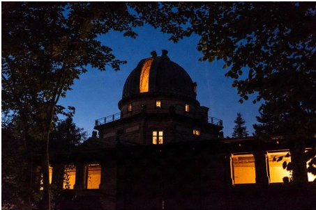
Figure 1: The Astronomical Observatory of Strasbourg and its large refracting telescope at night.

The "Galaxies, High Energy, Cosmology, Compact Objects & Stars" team (GALHE-COS) studies the formation and evolution of galaxies included our Milky Way in a cosmological context, considering their stellar population and dark matter dynamics and the retroactive effects of their central black hole. The objects it tackles can be Galactic and extra-Galactic X-ray emitting sources, compact objects like neutron stars of white dwarves, and Galactic active nuclei. Rodrigo Ibata, my supervisor, is part of this team as a research director at the CNRS and specializes on the local group, the Milky Way and dark matter. The will to acquire precise heliocentric distances, and so to better understand the 3D construction of the Universe around us and more particularly of the Milky Way, is what motivated my internship.