2.2. Infinite dilution activity coefficients
2.2.1. Definition
The activity coefficient of species in a solution is defined by
the following ratio:
(2-1)
where, is the fugacity of component in solution, its pure
component fugacity and, its
molar fraction. Activity coefficient is also defined as the
proportionality constant between the activity of a substance and its mole
fraction in a given solution.
(2-2)
In the study of phase equilibria and therefore the design and
optimization of separation processes, the concept of activity coefficient is
used rather than activity.
2.2.2. Importance and use of infinite dilution activity
coefficient data
The infinite dilution activity coefficient , also referred to as
limiting activity coefficient is the
limiting value of the activity coefficient of a solute when
its concentration tends towards zero. Alessi et al. (1991) defined the infinite
dilution region as one where each molecule of the solute is surrounded by
molecules of the solvent only. Only solute-solvent interactions take place.
This can be assumed for mole fractions ranging between 10-7 and
10-4, depending on components under investigation. The infinite
dilution region of solutions attracted much interest for couple of reasons
underlining its great importance (Raal and Mühlbauer 1998):
a) The system behavior in the very dilute regions is
instrumental in obtaining high purity products;
b) The most difficult and costly stage of a separation process
is the removal of the last traces of impurity;
c) The greatest departure from ideality occurs in the very
dilute regions;
d) Environmental concerns are based on the very dilute regions
in the gas phase which is air.
Sandler (1996) discusses theoretical and practical
applications of infinite dilution activity coefficient (IDAC) values in
chemical and environmental engineering. The most important ones that are
related to chemical engineering are listed below:
a) Synthesis, design and optimization of separation
processes;
b) Calculation of Henry`s law constants;
c) Predicting the existence of an azeotrope;
d) Development of predictive methods for
e) Characterization of behavior for liquid mixtures.
2.2.2.1. Synthesis, design and optimization of separation
processes
Separation is a critical stage in most of chemical processes
by virtue of its sensitive impact on the global cost, as well as the quality of
the product. One of the most important applications of IDACs is found in
separation processes. IDAC values are used in the preliminary selection of
solvent in view of extractive distillation, as well as, liquid-liquid
extraction (Tiegs et al. 1986). The potentially best separating agent, called
entrainer, is the one allowing the highest selectivity and capacity values. In
other words, when solvents are investigated to find out the most suitable
separating agent for a mixture containing two components and , their respective
IDAC
values in each solvent are determined. Equation (2-3) is then
used to calculate the selectivity at infinite dilution of each solvent with
respect to the system.
(2-3)
and represent the limiting activity coefficients of and
respectively in the solvent,
. is the limiting selectivity of solvent for the system
consisting of components and
. Thus, selectivity values at infinite dilution are important for
a preliminary selection of an
entrainer. A second quantity to look at is the
solvent capacity at infinite dilution, which is
numerically the maximum amount of species that can be dissolved
in the solvent.
(2-4)
Additionally, capacity reveals how much solvent is used during
the separation process. The greater the solvent capacity, the smaller the
amount of solvent used. In principle, the solvent to use as separating agent is
supposed to have the greatest value of both selectivity and capacity. But in
practice, a compromise is to be found, since these two quantities are in
inverse variation with respect to one another. A criterion that incorporates
both selectivity and capacity together
is called performance index, given by the product of these
properties (Kumar and Banerjee
2009). Thus, at infinite dilution,
(2-5)
The determination of permits one to evaluate the potential use of
solvents. Therefore, it
serves as a preselection criterion. Other criteria (Lydersen
1983) leading to the definitive choice of a solvent include: recoverability,
distribution coefficient, solvent solubility, density, interfacial tension,
viscosity, cost, corrosiveness, non-flammability, low toxicity, etc.
2.2.2.2. Calculation of Henry's law constants
There is a relationship between the Henry`s law constant of a
solute in a solvent and its limiting activity coefficient:
(2-6)
represents the Henry`s law constant for solute i in the
solvent and is the vapour pressure
of solute i at the temperature for which the IDAC is
determined. Equation (2-6) shows that
Henry`s law constants can be found
through IDAC values. In cases where the temperature of the
system is above
the critical temperature of the solute, the Henry`s law constant, rather than
the
ln e
8 i
l l 8
IDAC is useful (Eike et al. 2004). Design calculations for gas
separation applications commonly ln e j
involve the use of Henry`s law constants.
2.2.2.3. Predicting the existence of an
azeotrope
Conditions for the occurrence of an azeotrope in binary
systems can be established using infinite dilution activity coefficient data
(Gmehling and Möllmann 1998). For a system showing positive deviation from
Raoult`s law, an azeotrope with a temperature-minimum (pressure-maximum) takes
place when
(2-7) For a system exhibiting negative deviation from Raoult`s
law, an azeotrope with a temperature- maximum (pressure-minimum) takes place
when:
(2-8)
From equations 2-7 and 2-8, it obviously appears that the
knowledge of the IDAC values can help in predicting conditions leading to an
azeotropic mixture.
2.2.2.4. Development of predictive methods
for
Values of infinite dilution activity coefficient are important
for the development of new thermodynamic models, the adjustment of parameters,
as well as the expansion of the applicability for the existing group
contribution models (Gmehling 2003 and Nebig et al. 2009). With the aid of an
appropriate correlation, one can use infinite dilution activity coefficient
values to come up with VLE data in the intermediate concentration range.
Additionally, it is recommended to fit group interaction parameters
simultaneously to all available VLE, LLE and infinite dilution activity
coefficient experimental data (Weidlich and Gmehling 1987).
2.2.2.5. Characterization of behavior for liquid
mixtures
The infinite dilution activity coefficient value is an
indication of the nature of interactions between solute and solvent molecules
(McMillan and Mayer 1945). A high IDAC value is synonymous of weak
solute-solvent interactions i.e. low solubility (Cheong 2003). The IDAC value
is also a limiting measurement of the nonideality (Bao and Han 1995) of a
solution. For an
E
? ? G RT
E
? ?
/ ? H
ideal system, whereas a departure from ideality corresponds to
IDAC values greater or
RT 2
?? = T ??
smaller than unity.
2.2.3. Temperature dependence of activity
coefficient
The Gibbs-Helmholtz equation (2-9) depicts the effect of
temperature change on activity coefficient.
This leads to the following significant relations:
(2-10)
(2-11)
Using experimental ã8 data, the partial excess
enthalpy at infinite dilution for a given solute i,
can be directly obtained from the slope of a straight line
derived from equation (2-11), where is the gas constant. It only takes an
approximation of experimental values by the linear regression,
(2-12)
This procedure is widely used in the experimental section of this
thesis.
2.2.4. Predictive activity coefficient models
Predictive thermodynamic models are very important in separation
processes (Lei et al. 2008) as they allow:
a) A rapid solvent selection at reduced costs (Novak et al.
1987);
b) Accessing data that are difficult or impossible to obtain
experimentally;
c) The development of process simulators (Gmehling 2003).
It is beyond the scope of this study to review all the
thermodynamic models used to predict infinite dilution activity coefficients.
Only the most promising models used for systems involving ionic liquids are
dealt with in this section. The most successful models used by various
researchers to predict activity coefficients of various solutes in ionic
liquids can be classified into two categories:
a) Group contribution methods;
b) COSMO-based methods.
2.2.4.1 Group Contribution methods. (GCMs)
These methods are based on the group contribution concept
which assumes that the interaction energy of a system is the sum of functional
groups interaction energies, provided that groups are properly defined
(Gmehling 2009). Molecules are therefore split into smaller structures called
groups to which parameters are assigned. These activity coefficient models are
mostly based on the relationship between the latter and the excess free
energy.
The ASOG (Analytical Solution of Group) Model
The ASOG (Analytical Solution of Group) model was developed by
Derr and Deal (1969) who exploited previous works by Wilson and Deal (1962). It
was redefined by Kojima and Tochigi (1979) who modified several parameters in
order to account for the effect of temperature changes. In this method, the
expression of the activity coefficient is composed of two parts: the size
contribution term and the group interaction one. Go et al. (2007) used the ASOG
model to correlate experimental infinite dilution activity coefficient data of
n-octane, n-nonane and ndecane in the ionic liquid
4-methyl-n-butylpyridinium tetrafluoroborate in the temperature range
from 297 to 344 K. Their results were in good agreement with the experimental
measurements. Twelve interaction parameters related to three structural groups,
CH2, pyridinium and BF4 were determined.
The UNIFAC model and its modifications
After its publication by Fredenslund et al. (1975), the UNIFAC
(Uniquac Quasi-Chemical Functional Activity Coefficient) underwent a plethora
of revisions and extensions which are outlined in reviews by Lei et al. (2008)
and Castells et al. (1999).
The original UNIFAC, as stated by Lohmann and Gmehling (2001),
presented the following advantages:
a) Availability through commercial processes simulators;
b) Reliability in predicting VLE results;
c) Applicability over a wide range of mixtures.
The same authors highlight its weaknesses as follows:
a) Incorrect description of the temperature-dependence of the
activity coefficient and other related properties;
b) Unsatisfactory results when predicting properties in the
dilute region, as well as for asymmetric systems.
In an attempt to remedy these limitations, more advanced
versions of the UNIFAC model were developed, the most important ones being
UNIFAC (Dortmund) by Weidlich and Gmehling (1987) and UNIFAC (Lynby) by Larsen
et al. (1987). The modified UNIFAC (Dortmund) differs from the original UNIFAC
model in that it uses a different combinatorial part and it reliably takes into
account the temperature dependence of group interaction parameters. Its
developers introduced new van der Waals quantities as well. No thermodynamic
model can claim as much popularity as UNIFAC (Do). This is attributed to the
amount of research work and publications related to it in the last twenty
years. Moreover, around fifty companies and
institutions work actively in the UNIFAC Consortium to support
directly or indirectly its perfections. The Thermodynamics Research Unit, at
the University of KwaZulu-Natal is part of this organization. Successes
recorded in improving the predictability of properties using UNIFAC (Dortmund)
are presented in publications by Gmehling and Schiller (1993), Hansen et al.
(1991), Gmehling (1995), Gmehling et al.(1998), Gmehling et al.(2002), Gmehling
et al.(2009), Lohmann and Gmehling (2001), Wittig et al.(2001) and Jakob et al.
(2006). Recently, Prof. Gmehling`s group started to assess the predictive
ability of UNIFAC (Do) for systems involving ionic liquids. The parameter
matrix of this model has been expanded, allowing for the prediction of infinite
dilution activity coefficients of:
a) n-alkanes and alk-1-enes in [BMPyr] [BTI], [HMPyr] [BTI] and
[OMPyr] [BTI] (Nebig et al. 2009);
b) Methylcyclohexane and toluene in [HMIM] [BTI] (Liebert et al.
2008);
c) n-alkanes, benzene and toluene in [MMIM] [BTI] [BMIM] [BTI]
[HMIM] [BTI], as well as benzene and toluene in [BMIM] [BTI] (Nebig et al.
2007);
? ? d ?
d) n-alkanes, alk-1-enes, cycloalkanes, cycloalkenes, aromatics,
alcohols, ketones, esters, ethers and water in [HMIM][BTI], [OMIM][BTI],
[BMPyr][BTI];
e) The binary mixture of [BMIM] [BTI] and [EMIM] [BTI] (50:50
weight percent) (Kato and Gmehling 2005b).
It is clear that the parameter matrix remains very limited
when one looks at the number of ions involved in the structure of ionic
liquids. The major weakness of GCMs is their inability to deal with isomers,
proximity effects and systems involving groups for which experimental data have
never been compiled (Putnam et al. 2004).
2.2.4.2. COSMO-based methods
The conductor-like screening model (COSMO) is a predictive
method for thermophysical properties using a quantum chemical approach. Its two
most widely used variants for infinite dilution activity coefficients in ionic
liquids are COSMO-RS (The conductor-like screening model for real solvents),
developed by Klamt (1995) and COSMO-SAC (The conductor-like screening model,
solvation activity coefficients) (Lin and Sandler 2002). These two models
involve statistical thermodynamics, along with quantum chemical calculation
(Eckert and Klamt 2003). They require -profiles of molecules in the same manner
as group contribution methods rely on group interaction parameters. A -profile
is defined by Klamt and Eckert (2000) as a distribution function of the amount
of surface having a screening charge density between and
?. COSMO-based models are parameterized for 9 elements so far:
hydrogen, carbon, nitrogen, oxygen, fluorine, chlorine, bromine, iodine and
sulfur. They rely on a very small
number of parameters (Eckert and Klamt 2003) which are not
specific regarding molecules types or functional groups. This represents a
great advantage as compared to GCMs which involve a large number of functional
groups. Even components that have never been synthesized before can be studied
since no experimental data are needed to carry out predictions as shown by
Klamt et al. (1998). Long computation time and high computation costs are the
major disadvantages of these COSMO-based models. In a paper discussing
comparisons between COSMO-RS and GCMs, Grensemann and Gmehling (2005), taking
into account another article to which Klamt himself contributed (Putnam et al.
2004) reveal the following:
a) COSMO-RS achieves poor results in the applicability limits of
GCM`s, more especially, UNIFAC (Do);
b) COSMO-RS is advisable in cases of unknown GCMs parameters,
isomer and proximity effects.
This paper prompted a strong reaction from the developer of
COSMO-RS (Klamt 2005) who found its conclusions biased in order to clearly
favour the Modified UNIFAC (Do). From a neutral point of view, more time is
required to confirm whether COSMO-RS is inferior or superior to GCMs (Klamt and
Eckert 2008). More importantly, extensions are under way to improve both
models. Infinite dilution activity coefficients of a large spectrum of solutes
in some ionic liquids have been predicted using COSMO-RS. In a study on the
removal of thiophene from diesel oil (Kumar and Banerjee 2009), COSMO-RS
predictions of infinite dilution activity coefficient of alkanes, alk-1-enes
and cycloalkanes in [HMIM] [PF6], [HMIM] [BF4], [MOIM] [Cl] and [EMIM] [Tf2N]
are reported. The average absolute deviation of their predictions was found to
be 12% with respect to experimental data. Larger errors are observed in a
quantum chemical approach work by Sumon (2005) when predicting of toluene
and
heptane in a large number of ionic liquids. Other similar
predictive works (Banerjee and Khanna 2006, and Lei et al. 2007b) were in fair
agreement with experimental measurements, exhibiting the same range of
errors.
2.2.5. Experimental techniques for IDACs
measurements
Various experimental methods exist for determining infinite
dilution activity coefficients:
a) Gas-Liquid Chromatography (Letcher 1980);
b) Inert Gas Stripping Method (Leroi et al. 1977 and Richon et
al. 1980);
c) Headspace Analysis Method (Hussam and Carr 1985);
d) Indirect Headspace Chromatography. (Li and Carr 1993);
e) Dew Point Method (Eckert and Sherman 1996);
f) Differential Static Cell Method (Alessi et al. 1986);
g) Differential Ebulliometry Method (Gautreaux and Coates
1955);
h) Rayleigh Distillation Method (Dohnal and Horakova 1991).
The two methods used in this work, are the most popular ones
for ionic liquids. They are discussed here, with an emphasis on their
suitability for this class of solvents. A useful review paper by Kojima et al.
(1997) gives more details on other experimental techniques used for direct IDAC
measurements.
2.2.5.1. Gas liquid chromatography (GLC)
In this technique, the solvent, used as stationary phase, is
loaded onto the column. The solute, which is the mobile phase, is injected in a
carrier gas through the column. The eluted solute is detected and its retention
time, along with other experimental parameters, is used in an equation to
compute the IDAC. Gas-liquid chromatography can be used for IDACs of volatile
solutes in non-volatile or low volatility solvents. It is not applicable to
systems involving a mixture of solvents. Table 2-4 summarizes the advantages
and disadvantages of Gas-Liquid Chromatography.
Table 2-4: Advantages and disadvantages of the
Gas Liquid Chromatographic method
Advantages Disadvantages
Sample purity is not required The method is suited to low
volatility
or non-volatile solvents only
The method is rapid as many solutes can be injected at once
Reactive systems can be investigated
The IDAC of the solvent in the solute cannot be determined
2.2.5.2. The inert gas stripping technique.
(IGS)
In this method, a highly dilute solute is stripped from a
solution by a constant inert gas flow under isothermal conditions. The vapour
leaving the cell is periodically analyzed by gas chromatography. It is observed
that the peak area depicting the solute concentration in the vapour phase
decreases exponentially with time. Under this particular condition of
exponential dilution, the infinite dilution activity coefficient of the solute
in the solvent is related to the
decreasing rate of its corresponding peak area with time. The IGS
method is used to measure
of volatile solutes in non-volatile or volatile solvents.
Systems with solvent mixtures can be
investigated. The method is
alternatively called the dilutor technique, as well as continuous gas
extraction technique (Vitenberg 2003; Dobryakov and Vitenberg
2006). Table 2-5 presents the advantages and disadvantages of this
technique.
Table 2-5: Advantages and disadvantages of the
inert gas stripping method
Advantages Disadvantages
GC calibration is not required since only peak area ratios are
involved in calculations
A mixture of solvents can be investigated.
Systems with high volatility solvents can be measured
Many solutes can be investigated at once
Solutes must be purified.
Low volatility solutes are difficult to measure.
A good gas-liquid contact is critical to obtain reliable
results.
2.3. Advances in the design of IGS equipment 2.3.1. Major
developments in the use of the IGSM
Since its establishment by Leroi et al. (1977), the IGSM
underwent some improvements in terms of modernization of the analytical tool
(GC), temperature and pressure sensors, achievement of isothermal conditions
during experiments, etc. But the most important advance in this technique lies
in a better understanding of factors affecting the accuracy of measurements
provided by many research works. This resulted in various cell designs in order
to suit different types of systems. Bao and Han (1995) sum up the major
advances in the inert gas stripping technique as follows:
a) Establishment of the IGS technique by Leroi et al. (1977);
b) Correction by Duhem and Vidal (1978) for the liquid
concentration of the solute by taking into account its partition between the
two phases in the dilutor cell;
c) Modification of the dilutor cell structure by Richon and
coworkers (Richon et al. 1980 and Richon and Renon 1980);
d) Use of the two-cell technique in order to investigate low
boiling solvents. (Doleúal et al. 1981, and Doleúal and Holub
1985);
e) Extension of the technique to viscous or foaming systems by
Richon et al. (1985);
f) Further extension to mixtures containing food or oil
(Lebert and Richon 1984a, b). More recent developments involve the liquid
analysis gas stripping method (Hradetzky et al. 1990), the use of the inert gas
stripping technique for systems with ionic liquids ( Krummen et al. 2002) and
its extension to more delicate solvents of environmental interest involving
semi-volatile and surface tension solutes (Kutsuna and Hori 2008).
2.3.2. The number of cells required for IDAC
measurements
Either one or two cells can be used to measure infinite
dilution activity coefficients by the inert gas stripping method. The single
cell technique is suitable for systems with low volatility solvents and
relatively high volatility solutes. The double cell technique is required when
the solvent is a high volatile compound or mixture. In this variant, a
presaturation cell is used to saturate the stripping gas with the solvent
before the solute stripping process. This prevents any transfer of the solvent
from the liquid to the vapour phase which would lead to changes of the amount
of solvent in the dilutor cell. The single cell technique is appropriate to
systems involving ionic liquids since they are generally very high boiling
compounds and non volatile. Krummen et al. (2002) reported infinite dilution
activity coefficient data for n-alkanes and alk1-enes, cyclic hydrocarbons,
aromatic hydrocarbons, ketones, alcohols, and water in the ionic liquids
1-methyl-3-methylimidazolium bis (trifluoromethylsulfonyl) imide, 1-ethyl-3-
methylimidazolium bis (trifluoromethyl sulfonyl) imide,
1-butyl-3-methylimidazolium bis (trifluoromethylsulfonyl) imide, and
1-ethyl-3-methylimidazolium ethylsulfate in the temperature range between
293.15 K and 333.15 K. Activity coefficients at infinite dilution of alkanols
in the ionic liquids 1-butyl-3-methylimidazolium hexafluorophosphate,
1-butyl-3- methylimidazolium methylsulfate, [BMIM][MeSO4], and
1-hexyl-3-methylimidazolium bis(trifluoromethylsulfonyl) imide, [HMIM][Tf2N],
were measured by Dobryakov et al (2008). Using the same method, Nebig et al.
(2009) determined for n-alkanes and alk-1-enes in the
ionic liquids 1-butyl-1-methylpyrrolidinium bis
(trifluoromethylsulfonyl) imide, 1-hexyl-1- methyl pyrrolidinium bis
(trifluoromethylsulfonyl) imide and 1-methyl-1-octylpyrrolidinium bis
(trifluoromethylsulfonyl) imide. Kato and Gmehling (2005a, b) presented
infinite dilution activity coefficient data for seven solutes in the ionic
liquids 1-butyl-3-methylimidazolium bis (trifluoromethylsulfonyl) imide and
1-ethyl-3-methylimidazolium bis (trifluoromethylsulfonyl) imide using the
methods of gas liquid chromatography and the inert gas stripping technique.
Their results show a good agreement between the two methods.
2.3.3. Cell design parameters
Thermodynamic equilibrium between the gas leaving the dilutor
cell and the remaining liquid is instrumental in obtaining accurate infinite
dilution activity coefficient data.To achieve this, three conditions must be
met (Leroi et al. 1977):
a) Large total mass transfer area;
b) Sufficiently long contact time;
c) Good dispersion of bubbles in the liquid.
Studies mentioned in the two previous sections threw light on
these factors which affect the
performance of the IGSM:
a) Dispersion device;
b) Bubble rise height;
c) Stripping gas flow rate;
d) Bubble size;
e) Liquid viscosity;
f) Range of IDACs to be measured.
For accurate measurements of IDAC, it is essential to take
into account these factors when designing dilutor cells. The impact of each of
these parameters is briefly explained in the light of expressions derived by
Richon et al. (1980) which are reviewed in Chapter 3 of this thesis.
2.3.3.1. Dispersion device
In the original version of the method by Leroi et al (1977)
(See Figure 2-2), a fine porosity fritted glass was used as dispersion device.
Recently constructed dilutor cells are generally provided with stainless steel
capillaries with very small inner diameters. Stainless steel is known as a non
corrosive material. To ensure that the total mass transfer area is large, the
inert gas, generally helium or nitrogen, is dispersed into very small bubbles.
Capillaries must be in reasonable number and well spaced to avoid any bubble
coalescence. Dobryakov et al. (2008) designed a very small cell, of volume 5
cm3, with just a single capillary tube used as the dispersion
device.
2.3.3.2. Bubble rise height
The liquid level in the cell must be high enough for
sufficient contact time between the bubbles and the investigated solution. This
is a very important condition in view of attaining the required thermodynamic
equilibrium.
2.3.3.3. Stripping gas flow rate
Efficient solute mass transfer from the liquid phase to the
gaseous phase requires low inert gas flow rates as this results in longer
contact times. The optimum flow rate depends on the system under investigation.
It has been shown that when thermodynamic equilibrium has been attained between
the two phases inside the dilutor cell, measured infinite dilution activity
coefficients do not depend on the flow rate value. Additionally, the size of
bubbles is affected by the flow rate, increasing up when the flow rate is
increased. In previous works, experiments were performed with inert gas flow
rates ranging between some tenths to tens of cm3 (Kutsuna and Hori
2008, and Krummen et al. 2002)
2.3.3.4. Bubble size
The smaller the bubble size, the more efficient is the mass
transfer. In effect, when the inert gas is dispersed into the solution as small
bubbles, the total mass transfer area is increased. If bigger bubbles are used,
the height of the cell must be high enough to ensure a long residence time of
the gaseous phase in the solution.
2.3.3.5. Liquid viscosity
A high viscosity hinders mass transfer. Its other effect
consists of reducing the bubble rise and consequently allowing larger contact
times. The two effects with regards to mass transfer and equilibrium conditions
in the cell compensate each other. However, more sophisticated features need to
be incorporated in the design of the dilutor cell, more especially its stirrer,
for very viscous mixtures (Richon et al. 1985).
2.3.3.6. Range of IDACs to be measured
When very high infinite dilution activity coefficient values
have to be measured, large amounts of solute are stripped out of the solution
in a very short period of time, since there are very weak interactions between
the components involved in the mixture. If care is not taken, this will
compromise the attainment of equilibrium and reduce the mass transfer extent as
the contact time may be insufficient. It is not therefore surprising that the
worst agreement between infinite dilution activity coefficient data obtained
with the GLC method and the dilutor technique were observed for very high
activity coefficients (Leroi et al. 1977). The designer should take into
account the range of IDACs values the cell is supposed to deal with in order to
tune other parameters such as the height and the dispersion device.
2.3.4. Review of previous equilibrium cells
Various cell designs have been reported over the last forty
years as part of the inert gas stripping set up for the determination of
infinite dilution activity coefficient, Henry`s law constant and partition
coefficient. The most efficient ones, taken from the open literature are
reviewed. The various researchers who designed the cells discussed in this
section reported a good agreement with infinite dilution activity coefficient
data obtained by the GC method. And, reproducibilities better than 2% were
obtained. However, the reliability seemed to be compromised when very
high values had to be measured. The other issue of concern is the
determination of in
viscous mixtures.
2.3.4.1. Leroi et al. (1977)
Leroi et al. (1977) used the pyrex glass cell represented in
figure 2-2 to measure infinite dilution activity coefficient for n-hexane and
benzene in ten different nonvolatile solvents, including Nmethyl-2-pyrrolidone
(NMP), dimethylsulfoxide (DMSO), dimethylformamide (DMF), nitrobenzene,
ethylene glycol and hexadecane. A solution of volume 25 cm3
could be accommodated by the still and an experiment lasted one to two hours.
Solutes were introduced into the cell by means of a 10 syringe via the septum.
Inert gas flow rates ranged from 50 to
150 cm3 .min-1. To ensure accurate
measurements, liquid drop entrainment was limited by a dead space above the
solution. This gas phase volume was kept small enough to ensure accurate
measurements. The dispersion device consisted of a fine porosity fritted glass
disk as mentioned previously.
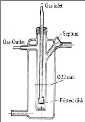
Figure 2-2: Dilutor cell constructed by Leroi et
al. (1977)
2.3.4.2 Richon et al. (1980)
Richon et al. (1980) designed the dilutor cell shown in figure
2-3, similarly to the one constructed by Leroi et al. (1977). Their major
improvements to the first cell include the following features:
a) Equal sized bubbles are introduced from the bottom by means
of fine capillaries;
b) A conical outlet gas collector is adopted to minimize liquid
entrainment.
They investigated infinite dilution activity coefficients of
alkanes from C1 to C9 in hexadecane. Experiments undertaken concluded that the
inert gas stripping method could be easily extended to Henry`s law constant
measurements. For Henry`s law constants greater than 30 atm., their work showed
the necessity to keep a very small and homogeneous vapour phase in the cell.
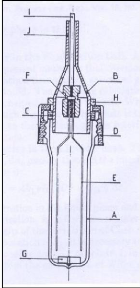
Figure 2-3: Equilibrium cell constructed by
Richon et al. (1980)
A - glass still body, B - conical collector of gas
outlet, C - gasket, D - plug, E - capillaries, F -
Teflon seal, G - magnetic
stirrer, H - metallic ring used to adjust the depth of the conical
collector
B in the still, I - tube for carrier gas inlet, J - gas outlet.
2.3.4.3. Richon and Renon (1980)
In this design, Richon and Renon (1980) abandoned the previous
conical shape in favour of a simpler shape as shown in figure 2-4. A
considerably reduced 1 cm high gas phase is kept above the solution inside the
dilutor cell. Their cell was used to determine infinite dilution activity
coefficients of light hydrocarbons in n-hexadecane, n-octadecane and 2, 2, 4,
4, 6, 8, 8- heptamethylnonane.
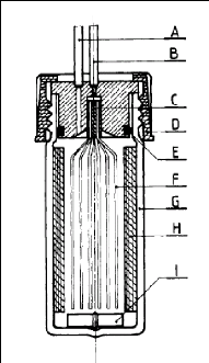
Figure 2-4: Dilutor cell used by Richon and
Renon (1980).
A - vapour phase outlet, B - inert gas inlet, C - Teflon seal,
D - plug, E - O-ring, F -
capillaries, G - glass still body, H - baffles, I
-magnetic stirrer.
2.3.4.4. Legret et al. (1983)
Legret et al. (1983) used the cell below (figure 2-5) to
determine partition coefficients which are related to activity coefficients at
infinite dilution. Their study involved some alkanes as solutes in the
methane/n-decane system. The pre-saturator and the dilutor cell were fitted
with 20 and 50 capillaries respectively. The capillary inner diameter was 0.3
mm for the pre-saturation cell and 0.1 mm for the dilutor cell. Both cells
contained 40 cm3 of solvent.
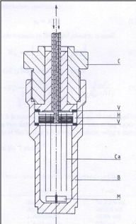
Figure 2-5: Dilutor cell design by Legret et al.
(1983)
B - body, C - cap, Ca - capillaries, H - capillary holder, M -
magnet, V - O?-ring
| 

