|
UNIVERSITÉ SCIENCES ET TECHNOLOGIES LILLE
1
THÈSE DE
DOCTORAT
présentée par Sylvain
LENOIR
Pour obtenir le grade de
DOCTEUR DE L'UNIVERSITÉ DE LILLE
1
Spécialité :
Écologie Marine
Filière
Doctorale : Géosciences, Écologie,
Paléontologie, Océanographie
École Doctorale :
Sciences de la Matière, du Rayonnement et de l'Environnement
Sujet de thèse :
Impact du réchauffement climatique sur la
distribution spatiale des ressources halieutiques le long du littoral
français:
observations et scénarios
Soutenue publiquement le 17 Janvier 2011
Numéro d'ordre : 40489
Membres du Jury :
Dr. Grégory BEAUGRAND
Chargé de Recherche, CNRS, Lille Directeur de
Thèse
Pr. Jean-Claude DAUVIN Professeur,
Université de Caen Directeur de Thèse
Pr. Chris Philip REID Chargé
de Recherche Principal, SAFHOS, Plymouth Rapporteur
Pr. Gilles BOEUF Professeur,
Université Pierre & Marie Curie Rapporteur
Pr. Alain LEPRÊTRE
Professeur, Université Lille1 Examinateur
Pr. Pierre CHARDY Professeur,
Université de Bordeaux1 Examinateur
Dr. Christophe LUCZAK Maitre de
conférences, Université d'Artois Examinateur
invité
Mme Dominique THOMAS
Responsable OP, CME, Boulogne-sur-Mer Examinatrice
invitée
Remerciements
Je tiens particulièrement à remercier le Dr.
Grégory Beaugrand, pour m'avoir accueilli au sein de son équipe
et m'avoir donné l'occasion et la chance de travailler à ses
côtés durant ces trois années de thèse. Je le
remercie pour la formation et les enseignements qu'il m'a donnés durant
toutes ces années, de même que pour m'avoir fait partager sa
vision globale de l'écologie.
Sa passion, sa persévérance, son amour de la
rigueur et du travail bien fait, souvent en confrontation avec ma
démarche un peu trop brouillonne, m'ont permis d'évoluer et
d'améliorer mes capacités au travail. Cela fait cinq ans
maintenant que j'apprends tous les jours à son contact, et
j'espère que cette relation enrichissante pourra continuer à
l'avenir.
Je le remercie, également, pour la confiance qu'il
a bien voulu me témoigner durant tout ce temps, pour sa patience, sa
bonne humeur, sa disponibilité et ses qualités humaines, ainsi
que son soutien dans les moments de baisses de motivations.
Je remercie, aussi, le Pr. Jean-Claude Dauvin pour avoir
codirigé ma thèse. Je le sais gré de m'avoir laissé
une grande liberté durant mes travaux de thèse tout en
étant toujours présent et disponible pour répondre
à mes questions et attentes. Son avis et son expertise ont
été très pertinents à des moments clefs de la
thèse. Il m'a, entre autres choses, permis d'intégrer
différentes réflexions scientifiques qui m'ont conduit à
avoir une approche plus complète de la recherche.
Je tiens à exprimer mes remerciements aux membres
du jury, qui ont accepté d'évaluer mon travail de
thèse.
Merci à monsieur Alain Leprêtre, Pr. des
universités de l'Université de Lille 1, d'avoir accepté de
présider le jury de cette thèse, et à messieurs les Prs.
Chris Reid de la SAFHOS et Gilles Boeuf de l'université de Paris VI,
d'avoir accepté d'être les rapporteurs de ce manuscrit.
Merci, également, à Madame Dominique Thomas
responsable OP à la CME, au Pr. Pierre Chardy de l'Université de
Bordeaux1 et au Dr. Christophe Luczak de l'Université d'Artois pour
avoir accepté d'examiner mon mémoire et de faire partie du jury
de thèse.
Je remercie le directeur de recherche monsieur
François Schmitt, directeur du LOG, de m'avoir accueilli au sein du
Laboratoire. De même que j'adresse mes remerciements à messieurs
M. Jean-Marie Dewarumez et au Professeur Sébastien Lefebvre, directeurs
de la station marine de Wimereux, pour m'avoir accueilli dans leurs
locaux.
Je remercie messieurs Vincent Touloumon et Éric
Gosselin, directeurs de la CME, pour m'avoir fait une place au sein des
Collectivités Maritimes Étaploises et pour m'avoir donné
la chance de mieux me rendre contre de la dureté et de la
complexité croissante du métier de marin pêcheur.
J'adresse mes remerciements à Éric
Lécuyer, son implication, ses connaissances et ses heures de travail
nous ont permis de mener à bien un projet qui a porté ses fruits.
Je remercie également le Docteur Christophe Luczak
pour ses différents avis éclairés au sujet du
régime alimentaire des oiseaux marins, en particulier, et pour
l'ensemble des conseils qu'il a pu me donner au cours de différentes
conversations.
Je remercie également tout le personnel de la
station marine de Wimereux qui de par sa sympathie et sa bonne humeur a
participé à la bonne ambiance générale à la
station marine. Mes remerciements vont également à tout le
personnel de la CME. J'ai eu de la chance, durant ces trois années, de
changer à plusieurs reprises de bureau au sein des locaux de la CME,
à chaque fois j'y ai retrouvé la même ambiance sympathique
et détendue. Je remercie également les marins pêcheurs du
Sainte Catherine Labouré, pour m'avoir accueilli à leur bord et
fait partager leur passionnant quotidien.
J'adresse un grand merci à tous mes amis et
collègues rencontrés durant la thèse avec qui j'ai pu
partager de bons moments de franches rigolades, d'anthologiques parties de foot
sur la plage de Wimereux, des découvertes culturelles, gastronomiques,
avec qui le monde a du être refais au moins.... Ho là... tellement
de fois.
J'adresse un merci tout particulièrement à
M. Éric Goberville, compagnon de route, compagnon de galères (je
devrais même mettre plusieurs « s »), compagnon de
foot (j'ai quand même la licence), compagnon de bureau (depuis peu),
compagnon de « chambré »... Voilà bien
longtemps, nos routes s'étaient croisées une première fois
à Bordeaux (même plusieurs fois grâce à la toute
nouvelle technologie d'APS !!!!!), pour se séparer par la suite.
Mais, apparemment, il était écrit que nous nous retrouverions et
qu'une chaleureuse (il y a le mot chat dedans, c'est clair) amitié nous
lierait ; les nombreuses péripéties et aventures qui
jalonnent notre parcours, dont je passe les détails, me font
espérer que cela continuera un bout de temps.
Un merci tout spécial au petit Gabriel qui s'est
exilé très loin de nous, merci pour ta passion et enthousiasme,
parfois un peur trop débordants peut-être pour le pantouflard que
je suis, mais ça fait partie de ton charme.
J'adresse également de chaleureux remerciements
à mes amis d'ici et d'ailleurs, Juliette, Céline (merci pour les
corrections) avec qui j'ai partagé les galères (fichue proprio)
et les joies de la colocation, Benjamin qui gentiment m'a confié la
recette sacrée de son Guacamole et s'en va bien trop loin de nous,
oOolivier et le Dr. Rombouts, Mikael et sa bonne humeur, David qui nous doit
toujours une séance nanards, Stella, Armonie, Pierre, Sophie, Gaspard,
Befa le chat, les amis qui me soutiennent de plus ou moins loin Audrey,
Virginie et Kevin, Adrien et Émilie, Magali et Jaï, Syndie,
Joëlle et Christophe.
Je remercie également mes soeurs, et
présente mes excuses pour ne pas avoir participé au
déménagement... Je me rattraperai, je ne sais pas encore
comment...
Un grand merci à mes parents qui m'ont toujours
soutenu et encouragé durant ma longue vie d'étudiant. Ils n'ont
jamais perdu espoir, bien qu'à un moment ils ont bien dû se
demander si j'allais un jour en finir avec les études...
Enfin j'adresse des remerciements tout particuliers
à Maud pour sa présence et ce qu'elle m'apporte au quotidien. Un
grand merci également, pour les heures et nuits passées à
m'aider à la rédaction de ce manuscrit.
La Terre n'est pas un don de nos parents. Ce sont nos enfants
qui nous la prêtent
Proverbe Amérindien
À Malicia, à celui ou celle qui arrive, et
à tous les autres.
Sommaire
INTRODUCTION GENERALE
1. Impacts du climat
3
1.1. Variabilités et Forçages
naturels
6
1.2. Impact du réchauffement climatique
7
2. La Niche Écologique et distribution
spatiale des espèces
9
3. Modèles d'habitats
11
4. Problématique et Objectifs
Généraux
13
CHAPITRE II: Un nouveau modèle pour
évaluer la probabilité de présence d'une espèce
basé uniquement sur des données de présence
1. Résumé du chapitre II
16
1.1. Avant-propos
16
1.2. Données utilisées
17
1.3. Méthode et Analyses
effectuées
19
1.4. Principaux résultats obtenus
20
1.5. Conclusion
21
2. Publication: A new model to assess the
probability of occurrence of a species based on presence-only data
22
2.1. Abstract
23
2.2. Introduction
24
2.3. Materials and Methods
26
2.4. Results
39
2.5. Discussion
47
CHAPITRE III: Distribution spatiale
modélisée des poissons marins et projections des changements dans
l'océan Atlantique Nord
1. Résumé du chapitre
53
1.1. Avant-propos
53
1.2. Données utilisées
54
1.3. Méthode et Analyses
effectuées
55
1.4. Principaux résultats obtenus
56
1.5. Conclusion
57
2. Publication: Modelled spatial distribution of
marine fish and projected modifications in the North Atlantic Ocean
58
2.1. Abstract
59
2.2. Introduction
60
2.3. Materials and Methods
62
2.4. Results
72
2.5. Discussion
79
Supporting information
84
Annexe: atlas climatique des ressources marines de
l'Atlantique Nordþ 104
CHAPITRE IV: Les effets du climat sur les proies
principales des oiseaux marins en mer du Nord
1. Résumé du Chapitre IV
3
1.1. Avant-propos
134
1.2. Données utilisées
135
1.3. Méthode et Analyses
effectuées
136
1.4. Principaux résultats obtenus
137
1.5. Conclusion
138
2. Publication: The effect of climate on the main
fish prey of North Sea seabirds
140
2.1. Abstract
141
2.2. Introduction
142
2.3. Material and Method
144
2.4. Results
147
2.5. Discussion
151
Supporting information 158
CHAPITRE V: Réchauffement climatique,
Calanus finmarchicus et la morue de l'Atlantique
1. Avant-propos
3
2. Données utilisées
167
3. Méthode et Analyses effectuées
170
4. Principaux résultats obtenus
171
5. Discussion
177
DISCUSSION, CONCLUSIONS, PERSPECTIVES
1. Discussion
181
1.1. Le modèle NPPEN
181
1.2. Impacts du réchauffement climatique sur
la distribution spatiale des poissons marins
185
1.3. Propagation du réchauffement climatique
le long du réseau trophique
189
2. Epilogue
192
2.1. Conclusions
192
2.2. Perspectives
194
REFERENCES BIBLIOGRAPHIQUES
INTRODUCTION GÉNÉRALELes
poissons marins constituent une ressource alimentaire essentielle à
l'humanité. D'après les chiffres de l'Organisation des Nations
Unies pour l'alimentation et l'agriculture (FAO), la production mondiale des
captures de pêches réalisées dans l'Océan1(*) en 2006 s'élevait
à 81,9 millions de tonnes. La plus grosse partie de cette production
(77%) était destinée à l'alimentation humaine (FAO, 2009;
Brander, 2007). Cette production n'a eu de cesse d'augmenter pour
répondre à l'accroissement de la population et de la demande en
poisson. L'accroissement de cette demande est induit par l'augmentation de la
part des protéines de poisson dans la quantité mondiale de
protéines animales ingérée par habitant de la
planète (Botsford et al., 1997 ; FAO, 2009). De plus,
toujours selon la FAO (2009), près de 43.5 millions de pêcheurs et
d'aquaculteurs travaillent et vivent directement des ressources halieutiques,
qui, en production, ont dégagé une valeur marchande
évaluée à 78,8 milliards de dollars US en 2006.
L'attrait commercial des ressources halieutiques a mené
les professionnels du secteur de la pêche à exercer une pression
croissante sur les stocks de poissons, aidés en cela par
l'industrialisation de leurs activités ainsi que par la sophistication
des instruments de détections et de captures. L'exploitation intensive,
à l'échelle industrielle, associée à une absence de
mesures de contrôle, de gestion et de conservation, a provoqué un
effondrement catastrophique de nombreux stocks de poissons marins (Myers et
al., 1997 ; Cook, 2000; Hutchings, 2000; Schrope, 2008). Des
espèces telles que la sardine en Californie (Hilborn & Walters,
1992; McFarlane et al., 2005) ou l'anchois au Pérou (Boerema
et al., 1965) ont vu, par le passé, leurs stocks pratiquement
s'épuiser, avant que des mesures de protections, par limitations des
captures, soient mises en places (McFarlane et al., 2005). Pour
d'autres espèces, l'interdiction d'exploitation a permis une
reconstruction partielle des stocks, comme par exemple celui du hareng en mer
du Nord (Fisher & Frank, 2002; ICES, 2005a). Malgré les mesures
prises, certains stocks, tels que ceux de la morue de l'Atlantique de
Terre-Neuve (Myers et al., 1996) ou de la mer du Nord (Cook et
al., 1997), ne se sont pas reconstitués au point de pouvoir
supporter une exploitation durable. L'état des lieux,
réalisé en 2006 par la FAO, indique que 80% des espèces de
poissons exploitées sont soit épuisées, soit
exploitées de manière excessive, ou proche de leur rendement
maximum, soit encore exploitées alors qu'en cours de relèvement
(FAO 2009).
Ce constat a conduit à la tentative de mise en place de
plans de gestion durable des ressources marines rendus possibles grâce
à une meilleure connaissance des impacts de la surexploitation sur les
populations de poissons (Pauly et al., 2005, Pauly, 2007). Comprendre
comment et pour quelles raisons les stocks de poissons fluctuent dans le temps
et l'espace, représente un défi que de nombreux scientifiques
tentent de relever (Steele & Henderson, 1984 ; Rosenzweig, 1995 ;
Jennings et al., 2001). Toutefois, l'étude seule des
conséquences de la surpêche sur une espèce ne suffit pas
pour expliquer les changements d'abondance et de répartition
géographique observés. Récemment, la complexité de
l'écosystème a été intégrée au sein
des stratégies de gestion des pêches (connues sous l'expression
anglaise « Ecosytem Based Fishery Management » EBFM ;
Cury et al., 2008). Par cette approche, la gestion d'une espèce
cible tient compte des relations de cette espèce avec son environnement,
son habitat et les autres espèces du milieu, ciblées ou non
(Pikitch et al., 2004).
Si par définition, la variabilité climatique,
qu'elle soit d'ordre naturelle ou induite par les activités humaines,
est incluse dans les EBFMs (Cury et al., 2008), le rôle et
l'importance de ce phénomène dans les fluctuations
spatio-temporelles des stocks de poissons font encore débat (Beaugrand
& Kirby 2010a). Pour certains scientifiques, il est impossible que seule la
variabilité du forçage climatique soit à l'origine de
disparitions ou d'épuisements de stocks de l'ampleur de ceux
observés (Pauly et al., 2002). Pour d'autres, les fluctuations
climatiques expliquent, en grande partie, celles répertoriées
dans la production (Brander et al., 2007 ; Brander, 2010;
Jennings & Brander, 2010), le recrutement (Jurado-Molina & Livingston,
2002 ; Beaugrand et al., 2003), la distribution, les migrations
et les abondances (Roessig et al., 2004; Perry et al.,
2005 ; Lehodey et al., 2006) des poissons exploités. En
conséquence, les effets de la pêche et du forçage
climatique, en particulier du réchauffement global, commencent à
être évalués et étudiés de concert (Rose,
2004; Mieszkowska et al., 2007 ; Kirby et al., 2009;
Perry et al., 2010; Planque et al., 2010).
Les modèles de dynamique des populations, ainsi que
ceux destinés à l'évaluation de l'état des stocks
exploitables (Hilborn & Walters, 1992 ; Rose, 2004 ; Andrew
et al., 2006), sont déjà nombreux et largement
utilisés. En revanche, le développement de modèles
permettant de comprendre, quantifier ou visualiser l'impact du climat sur les
ressources halieutiques, est beaucoup plus récent.
1. Impacts du climat
1.1. Variabilités et Forçages naturels
Les espèces marines et en particulier les organismes
ectothermes, que sont en grande majorité les poissons marins, sont sous
l'influence de leur environnement physique (Steele & Henderson, 1984 ;
Cushing, 1996; Daskalov, 1999). De fait, les stocks de poissons ont toujours
connu des fluctuations, dans le temps et dans l'espace, régies par la
variabilité des facteurs hydro-climatiques (Rosenzweig, 1995; Barange
& Harris, 2003). Avant même que l'homme n'exerce une pression sur les
stocks de poissons via les captures de pêche, ces espèces de
poissons connaissaient d'importantes variations naturelles (Poulsen, 2010), en
témoignent les séries d'abondance reconstituées de la
sardine du Pacifique au large de la Californie (Baumgartner et al.,
1992) ou du saumon rouge dans le Pacifique (Finney et al., 2000). En
2007, Enghoff et al. (2007) ont montré, à partir de
données sédimentaires provenant du Néolithique, et plus
précisément de la période comprise entre 7000 et 3000
avant J.C. dénommée « warm Atlantic period »,
qu'en mer Baltique l'ichtyofaune marine différait grandement de celle du
20e siècle. Cette différence s'explique par une
température moyenne estivale supérieure de 1,5 à 2,0
°C à la température moyenne estivale actuelle.
Les oscillations météo-océaniques telles
que l'Oscillation Nord Atlantique (NAO), représentent également
une source de variabilité du climat (Hurrell et al., 2001). Ces
patrons de variabilité, de par leur rôle majeur dans la
gouvernance des facteurs hydro-climatiques (e.g. régime des vents,
champs de pression, précipitations, températures), peuvent
exercer un effet significatif sur la variabilité du recrutement
(Dippner, 1997; Ottersen & Stenseth, 2001; Brander & Mohn, 2004; Stige
et al., 2006), cause primordiale de fluctuations des stocks de
poissons (Cushing, 1996). Dans l'océan Pacifique, les phases dites
« chaudes » (Trenberth 1997) de l'« El
Niño-Southern Oscillation » (ENSO) réchauffent les eaux
côtières de près de 8°C et modifient la
productivité du zooplancton. Un événement El Niño
crée ainsi un habitat caractérisé par un régime
thermique plus élevé provoquant des migrations latitudinales et
zonales des populations d'anchois et de sardines le long des côtes
d'Amérique du sud (Lehodey et al., 2006).
La puissance du forçage naturel peut s'exercer
également de façon ponctuelle, rapide, et inattendue, sous la
forme d'évènements climatiques exceptionnels de forte
magnitude : les changements de régimes2(*). Les conséquences de tels
phénomènes sur les poissons marins ont été mises en
évidence à de nombreuses reprises (e.g. Hare & Mantua
2000 ; Beaugrand, 2004; de Young et al., 2004 ; Rothschild
& Shannon, 2004 ; Beaugrand et al., 2008). Par exemple, suite
à un changement de régime au milieu des années 1970 dans
la baie de Pavlov en Alaska, les débarquements constitués
historiquement de crevettes rouges, ont laissé place à des
captures composées essentiellement d'espèces de gadoïdes et
de poissons plats. (Botsford et al., 1997). En 2006, Drinkwater
(Drinkwater, 2006) explique comment, de 1920 à 1930 dans l'océan
Atlantique, une période chaude a provoqué une extension rapide de
la limite nord de répartition de nombreuses espèces de poissons
telles que la morue de l'Atlantique, l'églefin ou le hareng.
L'élargissement brusque, vers des latitudes supérieures, de la
distribution des espèces indigènes s'accompagne, en
général, d'un phénomène de déplacement
latitudinal d'espèces dites « d'eau chaude »
à répartition plus subtropicale, comme le chinchard de
l'Atlantique, le turbot ou encore la plie cynoglosse (Reid et al.,
2001 ; Drinkwater, 2006).
1.2. Impact du réchauffement climatique
Le réchauffement climatique global, induit en grande
partie par les activités humaines, marque de son empreinte tous les
compartiments ou éléments fonctionnels de
l'écosphère (Parmesan & Yohe, 2003; Root et al.,
2003; Walther et al., 2005; Parmesan, 2006 ; Rosenzweig et
al., 2008; Beaugrand & Goberville 2010). Il affecte naturellement
l'océan qui a emmagasiné près de 84% du surplus de chaleur
ajoutée au système climatique (Levitus et al., 2005).
Cette accumulation d'énergie thermique a eu pour conséquence un
réchauffement global moyen de 0,06°C concernant les premiers trois
milles mètres de l'Océan, entre 1948 et 1998.
Une des conséquences les plus spectaculaires du
réchauffement planétaire est la réorganisation spatiale
des espèces. Des preuves évidentes montrent que le
réchauffement provoque le déplacement latitudinal des
espèces (Hughes, 2000 ; Parmesan & Yohe, 2003; Deutsch et
al., 2008; Muthoni, 2010). Cette réorganisation spatiale touche
également les espèces de poissons marins, exploitées ou
non (Perry et al., 2005; Brander et al., 2003). Les cas
d'apparitions d'espèces dites « tropicales » dans
les eaux tempérées et tempérées-froides de
l'Atlantique Nord-Est (Quero et al., 1998; Stebbing et al.,
2002; Beare et al., 2004a) illustrent bien ce phénomène.
D'autres espèces, familières des eaux de la mer du Nord telles
que l'entélure (Entelurus aequoreus Linnaeus, 1758),
ont vu leur abondance exploser et leur limite méridionale
supérieure de répartition s'étendre vers le Nord
(Kirby et al., 2006; Fleischer et al., 2007; Van Damme &
Couperus, 2008). Enfin, certains poissons, déjà durement
touchés par l'activité de pêche comme la morue de
l'Atlantique, sont repoussés de leur limite sud de répartition,
zones où les eaux deviennent trop chaudes (Beaugrand et al.,
2003; Mieszkowska et al., 2007).
Les mécanismes, par lesquels le réchauffement
climatique réorganise la distribution spatiale des espèces, sont
multiples et peuvent agir de façon directe comme indirecte (Brander
2007 ; Stige et al., 2010). L'augmentation de la
température de l'environnement a des conséquences directes qui
affectent les processus de croissance, de fécondité, et de
recrutement (Brander 2007), via notamment la limitation en oxygène des
organismes (Pörtner et al., 2001 ; Pörtner & Knust,
2007). Le réchauffement climatique perturbe également la
phénologie et les migrations saisonnières de certaines
espèces de poissons (Drinkwater, 2005). Indirectement, le
réchauffement climatique exerce son impact sur les poissons via le
réseau trophique (Beaugrand & Reid, 2003; Edwards & Richardson,
2004), et la composition des assemblages d'espèces de
l'écosystème dont ils dépendent pour leurs ressources
(Beaugrand et al., 2002b ; Beaugrand et al., 2010).
Kirby & Beaugrand (2009) ont également mis en évidence la
répercussion et l'amplification de l'impact du réchauffement du
climat à travers le réseau trophique depuis le phytoplancton
jusqu'aux poissons.
2. La Niche Écologique et distribution spatiale des
espèces
Le concept de « niche écologique »
est un sujet largement discuté dans la littérature (Leibold,
1995). De nombreuses et différentes interprétations de ce concept
existent (Peterson, 2001), de même que plusieurs adjectifs pour en
décliner ou affiner la définition (niche réalisée,
potentielle, fondamentale ; Guisan & Thuiller, 2005). En outre,
certains termes largement utilisés ont parfois des définitions
aux différences ténues ou des définitions qui chevauchent
d'autres notions telles que la notion d'habitat, d'environnement et d'enveloppe
écologique. Une certaine confusion peut résulter de cette
diversité d'appellations et d'interprétations (Kearney, 2006).
Si le mot « niche » a été
utilisé pour la première fois en écologie par le
naturaliste Joseph Grinnell (Grinnell, 1917) pour décrire les besoins et
contraintes environnementales d'une espèce, le concept de niche
écologique a été défini opérationnellement
par le zoologiste George Evelyn Hutchinson (Hutchinson, 1957). Celui-ci
décrit la niche écologique comme étant « un
volume à n dimensions, dans lequel chaque point correspond à un
état de l'environnement qui permettrait à une espèce
d'exister indéfiniment ». Selon cette définition,
l'identification de la niche écologique d'une espèce consiste
à identifier la réponse de cette espèce à
l'environnement (Leibold, 1995) ou, en d'autres termes, à identifier le
domaine de tolérance de l'espèce vis-à-vis des principaux
facteurs du milieu (Frontier & Pichot-Viale, 1993).
La niche, au sens d'Hutchinson, est un concept de type
mécanistique, reflet des relations entre des éléments du
biotope et de la biocénose, ce qui la différencie du concept de
niche habitat de Grinnell. De plus, à la niche conceptualisée par
Hutchinson, s'oppose le concept de niche d'Elton : « la niche
impact » (Leibold 1995). Du point de vue d'Elton (Elton, 1927), la
niche écologique décrit les effets immédiats de
l'espèce sur son environnement, elle précise le
« rôle » de l'espèce au sein de
l'écosystème. De par leur définition, ces deux concepts de
niche n'ont pas les mêmes types d'approches. La niche au sens
d'Hutchinson est utilisée lors d'une approche
autoécologique3(*) ou
physiologique, vouée à étudier la répartition
géographique des espèces à grandes échelles (Guisan
& Thuillier, 2005). La niche d'Elton quant à elle, est reliée
aux concepts de chaînes alimentaires et de niveau trophique d'une
espèce et donc aux relations impliquées à des
échelles plus locales (Guisan & Thuiller, 2005). C'est la
définition d'Hutchinson, très opérationnelle, qui a
été retenue dans le cadre de cette thèse.
Hutchinson (1957) introduit également les concepts de
niche fondamentale et de niche réalisée. La niche
représente le domaine de tolérance d'une espèce
vis-à-vis des facteurs environnementaux. Il s'agit d'une niche
théorique. En effet, rares sont les espèces occupant
l'intégralité de leur niche (Puilliam, 2000). Les interactions
biotiques, telles que la compétition ou la prédation, vont
contraindre l'espèce à occuper un espace différent de la
niche fondamentale (Helaouët & Beaugrand 2009) : il s'agit de la
niche réalisée. Cette niche réalisée est la niche
réelle, déterminable à partir de données
d'observations empiriques. Néanmoins, dans le cadre d'études
à macro-échelle, il est difficile de disposer de suffisamment de
données afin d'estimer les contours exacts de la niche
réalisée ou encore de déterminer l'ensemble des facteurs
décrivant cette niche. Pour ces diverses raisons, le principe de niche
écologique potentielle a été préféré,
dans ce travail de thèse. La niche écologique potentielle
représente une estimation de la niche réalisée, avec un
nombre de descripteur réduit.
La quantification de la relation niche écologique et
environnement constitue la base à partir de laquelle sont construits les
modèles d'habitat en écologie (Guisan & Zimmermann, 2000). Le
concept de niche potentielle, au sens d'Hutchinson, est
généralement utilisé dans les modèles d'habitats
à macro-échelle (Peterson, 2001; Pearson & Dawson, 2003),
afin d'évaluer les modifications biogéographiques potentielles,
passées et futures des espèces (Kearney et al.,
2004 ; Martínez-Meyers et al., 2004 ; Wiens et
al., 2009)
3. Modèles d'habitats
Les grands enjeux actuels que sont la conservation
d'espèces en danger d'extinction (Araújo et al., 2005;
Sanchez-Cordero et al., 2005; Brook et al., 2009), les
problèmes liés à l'invasion d'espèces exotiques
(Peterson, 2003; Peterson et al., 2008), ou encore la conservation de
la biodiversité (Martínez-Meyers et al., 2004;
Sanchez-Cordero et al., 2005; Hirzel et al., 2006),
nécessitent des outils d'aides à la décision et à
la prévision des changements susceptibles de survenir au sein de
l'écosystème marin. Ces outils numériques se retrouvent
sous les termes équivalents de modèle d'habitat, modèle de
niche écologique, ou modèle de distribution spatiale.
Bien que différant de par leur nom ou par la
procédure numérique qu'ils utilisent, les modèles
d'habitats fonctionnent sur un principe simple et commun : en partant de
la distribution connue d'une espèce, ils modélisent la niche
écologique potentielle dans le sens que lui confère Hutchinson
(1957), permettant ensuite de projeter cette niche dans un espace
géographique. Les enveloppes environnementales testées peuvent
provenir d'aires géographiques appartenant au passé (Bigg et
al., 2008) ou au présent (Hilbert & Ostendorf, 2001; Cheung
et al., 2008b), permettant ainsi d'évaluer et de calibrer les
modèles. Elles peuvent également représenter un
environnement futur potentiel. Dans ce cas, ce sont des scénarios
d'évolution du climat qui sont utilisés pour déterminer
quelle pourra être à l'avenir, la distribution spatiale des
espèces.
Trois grandes familles de modèles se distinguent : (1)
les modèles basés sur des données d'abondance ; (2)
les modèles basés sur la présence et l'absence ; (3)
les modèles basés uniquement sur des données de
présence.
Lorsque des données d'abondance ou de présence
et d'absence sont disponibles pour estimer la niche, il est possible d'utiliser
des modèles régressifs (Guisan et al., 2002) tels que
les modèles linéaires généralisés
(GLM ; McCullagh & Nelder, 1983), les modèles additifs
généralisés (GAM ; Hastie & Tibshirani, 1990),
les méthodes utilisant des modèles de réseaux de neurones
artificiel (ANN ; Mastrorillo et al., 1997), ou encore, les
arbres de classification et de régression (CART ; Thuiller, 2003 ;
Thuiller et al., 2003). Néanmoins, ces techniques
requièrent obligatoirement des variables quantitatives ou binaires
(présence et absence). Cette contrainte réduit le champ
d'utilisation de ces modèles. En effet, dans le milieu marin, les
certitudes à très grande échelle sur l'absence d'une
espèce sont rares. Dans ce cas, il convient d'utiliser des
modèles basés uniquement sur la présence pour
prédire, à partir de leur niche potentielle, la
répartition géographique des espèces (Carpenter et
al., 1993). Des procédures numériques, telles que BIOCLIM
(Busby, 1996), GARP (Genetic Algorithm for Rule-set Production ; Stockwell
& Noble, 1992; Stockwell et al., 2006), DOMAIN (Carpenter et
al., 1993), la méthode d'entropie maximale (MAXENT ; Phillip
et al., 2006) ou encore l'ENFA (Ecological Niche Factor
Analysis ; Hirzel et al., 2002), ont été mises en
place et sont largement utilisées. Dans le milieu marin, le RES
(Relative Environmental Suitability modèle ; Kaschner et
al., 2006) a permis de produire des cartes de distribution spatiale des
mammifères et a été adapté, par la suite, aux
poissons, pour créer le modèle AquaMaps utilisé par
FishBase (Kaschner et al., 2007).
Malgré tout, cette profusion de modèles ne
permet pas des projections de la distribution spatiale des ressources
halieutiques d'une façon à la fois robuste, facilement mise en
place et n'exigeant pas la normalité des variables. L'ENFA reste un
modèle paramétrique, DOMAIN et HABITAT fragmentent ou simplifient
la forme de la niche écologique lors de son estimation. Les
méthodes GARP et MAXENT nécessitent de définir
respectivement des règles de décision et des fonctions de seuil.
Le RES détermine la réponse des espèces aux facteurs du
milieu en utilisant une courbe de réponse de type
trapézoïdale, impliquant aussi le choix arbitraire de seuils.
4. Problématique et Objectifs Généraux
Ce manuscrit retranscrit les résultats des travaux
réalisés en thèse sous la forme d'une compilation
d'articles de recherche publiés, soumis ou en préparation.
Le premier objectif était de créer un
modèle d'habitat, appelé le Non Parametric Probabilistic
.Ecological Niche (NPPEN) modèle, basé sur le concept de niche
écologique d'Hutchinson, permettant de cartographier la niche et la
distribution spatiale potentielle des espèces de poissons marins. Ce
modèle se devait d'être à la fois simple, robuste,
non-paramétrique et se baser uniquement sur des données de
présence. Le résultat recherché devait nous permettre de
cartographier la distribution spatiale potentielle passée,
présente et future des poissons à partir d'un faible nombre de
descripteurs : la température de surface, la bathymétrie, la
salinité de surface et le type de sédiments. Le but final
étant d'utiliser ce modèle pour formuler des scénarios
potentiels d'évolution des ressources marines, exploitées ou non,
sur la base des scénarios d'évolution du climat du Groupe
d'Expert Intergouvernemental sur l'Évolution du Climat (GIEC). Le cas de
la morue de l'Atlantique (Gadus morhua Linnaeus, 1758) a
été étudié.
Le deuxième objectif consistait à tester le
modèle NPPEN sur une multitude d'espèces marines à la
distribution et aux exigences environnementales différentes. Le but
était d'évaluer l'impact du changement climatique sur la
distribution spatiale des poissons. L'étude s'est focalisée, dans
un premier temps, sur le calcul des gains et pertes potentiels d'habitat (en
km²) de huit espèces de poissons, exploitées ou non dans
l'océan Atlantique Nord. Dans un second temps, un atlas a
été produit en partenariat avec des professionnels de la
pêche, retraçant les changements potentiels de répartition
géographique de 51 espèces marines (poissons, crustacés et
céphalopodes) jusqu'en 2100. Ces projections permettront aux
professionnels de la pêche de prévoir et d'anticiper les
changements potentiels de leurs ressources.
Un troisième objectif consistait à (1)
modéliser, grâce à NPPEN, les changements passés et
actuels des probabilités de présence de trois espèces de
poissons en mer du Nord (zone CIEM 4) : le lançon nordique
(Ammodytes marinus Raitt, 1934), le sprat européen
(Sprattus sprattus Linnaeus, 1758) et l'entélure (Entelurus
aequoreus Linnaeus, 1758) et à (2) évaluer les
conséquences de ces changements sur certains prédateurs
supérieurs: les oiseaux marins. L'objectif était également
d'estimer si, dans le futur, des espèces de poissons à
affinités plus méditerranéennes, ou provenant des eaux
nord-africaines, telles que l'anchois européen (Engraulis
encrasicolus Linnaeus, 1758) et la sardine européenne (Sardina
pilchardus Walbaum, 1792), pouvaient constituer une alternative aux
espèces habituellement consommées par les oiseaux marins.
Enfin, un quatrième objectif consistait à
évaluer l'effet de l'incorporation d'un facteur biotique (Calanus
finmarchicus Gunnerus, 1770) sur la modélisation de la distribution
spatiale de la morue. Les modélisations de la niche écologique et
de la distribution spatiale de cette espèce, avec et sans incorporation
de C. finmarchicus, ont été comparées. Suite
à cette étude, l'évolution à long-terme de la
probabilité de présence de la morue a été
examinée dans trois écorégions marines (la région
de Terre-Neuve, la mer du Nord et l'Islande) pour prédire la
réponse régionale de la morue face au réchauffement
climatique global.
Les principaux résultats sont ensuite discutés
dans un cinquième et dernier chapitre. Trois axes y sont principalement
développés :
(1) une évaluation, par comparaison avec d'autres
modèles d'habitats déjà existants et utilisés par
la communauté scientifique, des capacités, avantages et
faiblesses du nouveau modèle d'habitat NPPEN;
(2) une discussion autour des conséquences
passées et attendues du réchauffement climatique sur la
distribution spatiale des poissons en Atlantique Nord et une comparaison avec
les mouvements biogéographiques attendus et observés pour
d'autres espèces de communautés différentes (Parmesan
& Yohe, 2003) ;
(3) l'impact des réponses des assemblages de poissons
sur certaines espèces d'oiseaux marins.
.
CHAPITRE II
Un nouveau modèle pour évaluer la
probabilité de présence d'une espèce basé
uniquement sur des données de présence
1. Résumé du chapitre II
1.1. Avant-propos
Le changement global, et plus particulièrement le
réchauffement climatique, ont un impact fort sur les organismes vivants
qui peuplent les milieux terrestres et aquatiques (Parmesan & Yohe, 2003;
Intergovernmental Panel on Climate Change, 2007a). Les espèces marines,
en grande majorité thermo-conformes, sont directement impactées
par le réchauffement des océans. Les conséquences de
l'augmentation des températures sur ces organismes sont multiples
(Edwards & Richardson, 2004; Stempniewicz et al., 2007; Brander,
2007). Parmi celles-ci, un phénomène de réorganisation
spatiale des espèces est observé (Brander et al., 2003;
Perry et al., 2005). Dans l'hémisphère Nord, de plus en
plus d'espèces sont observées à des latitudes
supérieures à leur limite nord de répartition habituelle
(Beaugrand et al., 2002a,b ; Harris et al., 2007) ou
voient leur abondance exploser, là où elles n'étaient que
rarement observées auparavant (Kirby et al., 2006; Van Damme
& Couperus, 2008).
Si les effets du changement climatique sur la distribution
spatiale des espèces sont de mieux en mieux connus et observés,
il est à l'heure actuelle impossible de prédire qu'elle sera
cette distribution spatiale à grande échelle dans le futur. Les
outils capables de formuler des prédictions, des scénarios
d'évolution potentielle de la répartition spatiale des
organismes, en réponse au réchauffement climatique, sont soit mal
utilisés (les limitations de ces outils ne sont pas prises en compte)
soit manquants (Pearson & Dawson, 2003).
Dans cette étude, nous partons du principe qu'une
espèce cherche à se maintenir dans un environnement en
conformité à sa niche écologique, au sens d'Hutchison
(Hutchinson, 1957). Par conséquent, nous nous proposons de
développer et de tester un modèle, le modèle
Non-Parametric Probabilistic Ecological Niche (NPPEN), qui évalue dans
quelle mesure un espace géographique (passé, présent ou
potentiel futur) peut fournir un espace environnemental accueillant pour une
espèce (Peterson, 2001). En d'autres termes, ce modèle
évalue l'appartenance d'un point géographique,
représenté par ses conditions environnementales, à la
niche écologique de l'espèce.
Ce type de modèle existe déjà. Toutefois,
différentes limitations, telles que le besoin absolu de données
de présence et d'absence, la contrainte de normalité des
variables, ou encore la nécessité d'utiliser un grand nombre de
descripteurs, rendent leur utilisation peu adaptée dans le cadre
d'étude à très grande échelle. Le NPPEN cumule les
avantages de ne requérir que des données de présences,
d'être non-paramétrique, et de pouvoir travailler de façon
robuste avec un nombre relativement faible de descripteurs.
Le modèle NPPEN sera appliqué sur une
espèce emblématique de l'Atlantique nord : la morue de
l'Atlantique (Gadus morhua, L.). Cette espèce est un poisson
d'un grand intérêt commercial, très largement
exploité. De fait, sa reproduction, sa dynamique des stocks, sa biologie
et sa distribution spatiale, ont très souvent été
étudiées et comprises. De même, ce gadoïde est
certainement celui pour lequel le plus de données d'observations,
utilisables, sont disponibles. Enfin, les signes d'un changement, lié au
réchauffement climatique, de la distribution spatiale de cette
espèce ont déjà été observés
(Beaugrand et al., 2003; Drinkwater, 2005; Beaugrand & Kirby,
2010b). De tels éléments font de cette espèce le candidat
idéal pour tester les compétences du NPPEN en termes de
modélisation spatiale passée, présente et future,
basée sur différents scénarios d'évolution du
climat.
1.2. Données utilisées
? Données abiotiques
Trois paramètres physiques ont été
utilisés pour cette étude : la température de surface
(SST), la bathymétrie et la salinité de surface (SSS) (Fig.
II.1).
Les données SST utilisées pour modéliser
la distribution spatiale de la morue de l'Atlantique de 1960 à 2005
proviennent de la base de données « International
Comprehensive Ocean-Atmosphere Data Set » (ICOADS,
http://icoads.noaa.gov;
Woodruff et al., 1987). Celles utilisées pour modéliser
les probabilités de présence, de 1990 à 2100, sont issues
de différents scénarios d'évolution du climat :
· scénarios SRES (Special Report on Emissions
Scenarios) A2, B2, produits du modèle ECHAM4 (EC pour European Center
and HAM pour Hamburg; (Roeckner et al., 1996),
· scénarios d'évolution SRES B1, A1B et les
scénarios COMMIT et PICNTRL, sorties du modèle HadCM3 (Hadley
Centre Coupled Model, version 3 ; Gordon et al., 2000),
· scénario d'évolution 1PTO4x
proposé par le modèle HadGEM1 (Hadley Centre Global Environmental
Model, version 1).
Les données de bathymétrie ont été
obtenues à partir de la « carte de bathymétrie de
l'océan global » (Smith & Sandwell, 1997), elle-même
construite grâce à des sondages acoustiques effectués sur
des navires et des relevés satellitaires.
Les valeurs annuelles de SSS utilisées (correspondant
à une moyenne entre 0 et ?10m) proviennent de la climatologie de Levitus
(Levitus, 1982), complétées par les données du Conseil
International pour l'Exploration de la Mer (CIEM, via le site internet
http://www.ices.dk), plus
précises en zones côtières.
L'aire géographique couverte par les trois variables
s'étend des latitudes 30,5°N à 70,5°N et des longitudes
80,5W à 70,5E (Fig. II.1 et Fig. II.2). Sur cette zone, les valeurs des
trois variables sont interpolées de façon bilinéaire, avec
une résolution de 0,1° longitude x 0,1° de latitude. Ainsi,
une grille environnementale couvrant l'Atlantique Nord est construite pour les
paramètres bathymétrie et SSS. Concernant les SST, une grille est
calculée annuellement pour la période 1960-2005 et pour les
décennies futures.
? Données biotiques
Les données de présence de la morue de
l'Atlantique (Gadus morhua, L.) proviennent de la base de
données en ligne FishBase (
http://www.fishbase.org) (Froese
& Pauly, 2009), complétée avec des données provenant
du Conseil International pour l'Exploitation de la Mer (CIEM ; ICES,
2005b, 2007), de la littérature et des connaissances scientifiques sur
la distribution spatiale de cette espèce (Brander et al.,
2006 ; Heath & Lough, 2007). Ces observations sont datées et
géo-référencées ; elles constituent un jeu de
données de 62160 observations (Fig. II.2).
1.3. Méthode et Analyses effectuées
? Méthode
Développement et définition du modèle
NPPEN à partir du modèle MRPP (Mielke et al., 1981;
Beaugrand & Helaouët, 2008) et choix d'une distance adaptée
(Mahalanobis, 1936) (Fig. II.3).
? Analyse 1
Une comparaison graphique entre les performances du
modèle basé sur la distance généralisée de
Mahalanobis et la distance de corde a été réalisée.
Dans le 1er cas, les deux paramètres environnementaux fictifs
utilisés étaient non-corrélés; dans le
2e cas, ils étaient très fortement
corrélés.
? Analyse 2
À partir des données brutes d'observation et
d'homogénéisation, les préférendums de la morue de
l'Atlantique ont été estimés pour chacun des
paramètres.
? Analyse 3
Le modèle est utilisé pour caractériser
la niche écologique potentielle de la morue de l'Atlantique comme une
fonction des paramètres SST, bathymétrie et SSS. Par la suite, la
conformité à la niche potentielle estimée, des enveloppes
environnementales, passées, présentes et futures de l'Atlantique
Nord (basées elles aussi sur SST, bathymétrie et SSS), a
été testée. A partir de ce test, des projections de la
distribution spatiale de cette espèce sur ces enveloppes ont
été réalisées.
1.4. Principaux résultats obtenus
? Analyse 1
Dans le cas de descripteurs environnementaux
non-corrélés, les résultats du modèle basé
sur des distances différentes (distance de Mahalanobis et distance de
corde) sont équivalents. Par contre, dans le cas de facteurs
environnementaux très corrélés, le modèle NPPEN
basé sur la distance de Mahalanobis est plus performant pour produire
une distribution spatiale potentielle proche de la distribution spatiale
réelle (Fig. II.4)
? Analyse 2
La morue de l'Atlantique est une espèce subarctique qui
est présente pour des SST se situant entre 2 et 17 °C, avec une
fréquence maximale d'observations proche de 8°C. Ce poisson
préfère les eaux des régions néritiques. Sa
bathymétrie de prédilection se situe vers ?200 m et il est
rarement observé quand celle-ci est inférieure à ?800 m.
En accord avec la nature euryhaline de l'espèce, les exigences de la
morue en terme de SST s'étalent entre les valeurs 7 et 36, avec un mode
observé vers 34.
? Analyse 3
Le modèle NPPEN permet, à partir des
données d'observations, de reconstruire une niche potentielle qui se
rapproche de la forme Gaussienne attendue (Fig. II.6). Cette niche potentielle,
correctement estimée, permet d'obtenir une cartographie de la
distribution spatiale de la morue de l'Atlantique très proche de celle
connue (Fig. II.7). Toutefois, l'estimation de la présence de
l'espèce, en bordure de niche, semble sous-estimée.
L'évolution passée de la répartition
spatiale de la morue de l'Atlantique, estimée par le modèle,
retranscrit bien les modifications réellement observées depuis
les années 1960 : une baisse de la probabilité de
présence en limite sud de la répartition de l'espèce et
une augmentation de la probabilité de présence en limite nord de
cette répartition (Fig. II.7). L'évolution future, et à
long terme, de la répartition spatiale de Gadus morhua,
modélisée suivant différents scénarios, montre, un
potentiel déplacement horizontal général vers le nord des
populations de ce poisson. L'intensité et l'incertitude de ce
déplacement sont fonctions de l'intensité et de l'incertitude des
scénarios utilisés (Figs. II.8 et II.9).
1.5. Conclusion
Le nouveau modèle NPPEN, appliqué à
l'échelle de l'Atlantique Nord, est capable de fournir des cartes de
distribution spatiale de l'espèce Gadus morhua, et ce avec
l'avantage de n'avoir besoin que des données de présence. Ce
modèle étant non-paramétrique, il s'affranchit
également du besoin de normalité des variables.
Le NPPEN explique la chute prononcée de l'abondance de
la morue en mer du Nord depuis les années 1960. Il se
révèle ainsi très utile pour évaluer les
changements futurs de la répartition géographique des
espèces, dans le contexte du changement climatique, en fonction de
scénarios d'évolution du climat. Ce modèle constitue un
nouvel outil d'aide à la gestion durable des stocks de la morue de
l'Atlantique.
2. Publication: A new model to assess the probability of
occurrence of a species based on presence-only data
A new model to assess the probability of occurrence of
a species based on presence-only data
G. Beaugrand, S. Lenoir, F. Ibañez, C. Manté
Marine Ecology Progress Series, 2011.(In press)
2.1. Abstract
This study aims to describe a new nonparametric ecological
niche model for the analysis of presence-only data, which we use to map the
spatial distribution of Atlantic cod and project the potential impact of
climate change on this species. The new model, called the Non-Parametric
Probabilistic Ecological Niche (NPPEN) model is derived from a test recently
applied to compare the ecological niche of two different species. The analysis
is based on a simplification of the Multiple Response Permutation Procedures
(MRPP) using the Generalised Mahalanobis distance. For the first time, we
propose to test the generalized Mahalanobis distance by a non-parametric
procedure so avoiding the arbitrary selection of quantile classes to allow the
direct estimation of the probability of occurrence of a species. The model
NPPEN was applied to model the ecological niche (sensu Hutchinson) of
Atlantic cod and therefore its spatial distribution. The modelled niche
exhibited high probabilities of occurrence at bathymetry ranging from 0 to 500
m (mode between 100 m and 300 m), at annual sea surface temperature from
-1°C to 14°C (mode between 4°C and 8°C) and at annual sea
surface salinity ranging from 0 to 36 (mode between 25 and 34). This made the
species a good indicator of the subarctic province. Current climate change is
having a strong effect on North Sea cod and may have also reinforced the
negative impact of fishing on stocks located offshore of North America. The
model shows a pronounced effect of current climate change on the spatial
distribution of Atlantic cod. Projections for the coming decades suggest that
cod may eventually disappear as a commercial species from regions where a
sustained decrease or collapse has already been documented. In contrast, the
abundance of cod is likely to increase over the Barents Sea.
Keywords: Ecological Niche Models; Multiple
Response Permutation Procedure; Generalised Mahalanobis distance; Ecological
niche; The Atlantic cod
2.2.
Introduction
The effects of climate change on living systems in both the
terrestrial and the marine realms are now well documented (Parmesan &
Matthews 2006, Intergovernmental Panel on Climate Change 2007a). In the marine
biosphere, current climate change is affecting the abundance, spatial
distribution and the phenology of species and altering prey-predator
interactions (Beaugrand et al. 2002, Beaugrand et al. 2003, Edwards &
Richardson 2004). The effect of climate change is seen from phytoplankton (Reid
et al. 1998) to zooplankton (Beaugrand et al. 2007) and fish (Brander et al.
2003, Perry et al. 2005), and translates from the physiological to the
ecosystem level (Pörtner & Farrell 2008) affecting coupling between
systems (i.e. bentho-pelagic coupling; (Reid & Edwards 2001, Kirby et al.
2008). Pronounced climate change may become a confounding factor of fishing and
both driving forces may act in synergy to precipitate the collapse of fish
stocks around the world (Beaugrand & Kirby 2010b, a). To better evaluate
the effect of climate on a species, it is essential to know its spatial
distribution; this information is often lacking in the marine realm.
One way to evaluate the spatial distribution of a species is
to use Ecological Niche Models (ENMs). ENMs, also known as bioclimatic
envelopes, are being more frequently used in the context of global change and
are often based on the concept of the ecological realised niche described by
Hutchinson (Hutchinson 1957). The realised niche is the environmental envelop
in which a species can be found when the effect of dispersal and interspecific
relationships are considered. ENMs have been used in conservation to manage
endangered species (Sanchez-Cordero et al. 2005), to predict the responses of
species to climate change (Berry et al. 2002), to forecast past distribution
(Bigg et al. 2008) and to estimate the potential invasion of a non-native
species (Peterson & Vieglais 2001). When quantitative data are available,
regression techniques such as Generalised Linear Models (GLMs; (McCullagh &
Nelder 1983) or Generalised Additive Models (GAMs; Hastie & Tibshirani
1990), ordination or neural networks have been frequently used (Guisan &
Zimmermann 2000, Guisan & Wilfried 2005). When only binary
(presence-absence) data are available there are far fewer techniques that can
be applied (regression techniques such as GAMs can still be utilised).
Traditional models such as BIOCLIM (based on multilevel rectilinear envelope)
and DOMAIN (based on point-to-point similarity metric) (Carpenter et al. 1993)
tend to be relatively simple, although more sophisticated models have been
developed recently such as Ecological Niche Factor Analysis (ENFA; and MAXENT
(Philips et al. 2006), which are based upon Principal Component Analysis (PCA)
and the principle of maximum entropy, respectively.
The objective of this study is to describe a new nonparametric
ENM adapted to presence-only data. This technique is based on a modified
version of the Multiple Response Permutation Procedure (MRPP; Mielke et al.
1981) using the Generalised Mahalanobis distance (Ibañez 1981). First, a
rationale is presented and the technique described. Second, a simple example of
a calculation based on simulated data illustrates the technique and the use of
the generalised Mahalanobis distance is justified. Third, we use the technique
to model the ecological niche of the Atlantic cod and map its probability of
occurrence. Then, we project the probability of cod occurrence for the middle
and the end of the 21st century based upon IPCC scenarios for changes in sea
surface temperature.
2.3. Materials and
Methods
? Physical data
Bathymetry data were obtained from a global ocean bathymetry
chart (1 degree longitude x 1 degree latitude) (Smith & Sandwell 1997);
this dataset is among the most complete, high-resolution image of sea floor
topography currently available. The chart was constructed from data obtained
from ships with detailed gravity anomaly information provided by the satellite
GEOSAT and ERS-1 (Smith & Sandwell 1997). Bathymetry data were considered
because the spatial distribution of Atlantic cod, which occurs mainly over
continental shelves (Sundby 2000), is explained partially by this parameter.
Salinity has a strong impact of the distribution of most
fishes. Annual Sea Surface Salinity (SSS, average values between 0 and 10
meters) data were obtained from the Levitus' climatology (Levitus 1982). ICES
data were used to complete the Levitus dataset in coastal regions where there
was no assessment of annual SSS (e.g. some regions of the eastern English
Channel). ICES data were downloaded from http://www.ices.dk. We did not include
temporal changes in salinity because the parameter is not at present well
assessed in the Atmosphere-Ocean General Circulation (AO-GCM) models (Martin
Visbeck, Personal Communication). Furthermore, the spatial variance in the
salinity is much more pronounced than the temporal variance.
The spatial distribution of cod is affected by temperature
(Brander 2000, ICES 2007). Sea Surface Temperature (SST; period 1960-2005) data
originated from the database International Comprehensive Ocean-Atmosphere Data
Set (ICOADS, longitudes with a spatial resolution of 1° longitude x
1° latitude;
http://icoads.noaa.gov) (Woodruff
et al. 1987). An annual mean was calculated for the period 1960-2005. Data on
SST were considered as this parameter has strong impact on the spatial
distribution of cod (Brander 2000, ICES 2007). The use of SST to assess the
niche of adult cod assumes that climate exerts its major influence on cod
through the effects of temperature on larval development and plankton food
availability since the pelagic larval stage is a critical life cycle phase
affecting recruitment (Beaugrand & Kirby 2010b, a).
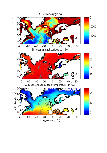
Figure II.1 : Spatial distribution of
bathymetry (A), mean annual sea surface salinity
(B) and mean annual sea surface temperature (C).
Isobaths 200m (dark grey line) and 2000m (light grey line) are
indicated.
To assess the potential impact of changes in SST, data
(1990-2100) from the Atmosphere-Ocean General Circulation Model (AO-GCM) ECHAM
4 (EC for European Centre and HAM for Hamburg; (Roeckner et al. 1996) were
used; these data are projections of monthly skin temperature equivalent above
the sea to SST (http://ipcc-ddc.cru.uea.ac.uk). Data used here are modelled
data based on scenario A2 (concentration of carbon dioxide of 856 ppm by 2100)
and B2 (concentration of carbon dioxide of 621 ppm by 2100) (Intergovernmental
Panel on Climate Change 2007b). Scenario SRES (Special Report on Emissions
Scenarios) A2 supposes an increase of CO2 similar to that currently
observed. Scenarios SRES A2 and B2 reflect world populations of 15.1 and 10.4
billion people in 2100, respectively (Intergovernmental Panel on Climate Change
2007b).
We also used data from the model HadCM3 (Hadley Centre Coupled
Model, version 3) (Gordon et al. 2000). Both scenarios SRES A1B and B1 were
used. Scenario A1B reflects a world of rapid economic growth, low population
growth and rapid introduction of new and more efficient technology whereas
scenario B1 reflects a world with rapid introduction of resource-efficient
technologies (Intergovernmental Panel on Climate Change 2007b). Two non-SRES
scenarios were also utilised: PICTL (i.e. experiments run with constant
pre-industrial levels of greenhouse gasses) and COMMIT (i.e. idealised scenario
in which the atmospheric burdens of long-lived greenhouse gasses are held fixed
at the 2000 level). The model HadGEM1 (Hadley Centre Global Environmental
Model, version 1) was also used with the non-SRES scenario 1PTO4x (1% to
quadruple) in which greenhouse gasses increase from pre-industrial levels at
rate of 1% per year until the concentration has quadrupled and become constant
thereafter (Johns et al. 2006). This is the more pessimistic of all scenarios
considered here. Therefore, a total of 7 scenarios (A2, B2, A1B, B1, PICTL,
COMMIT and 1PTO4X) was used from 3 different AO-GCMs (ECHAM4, HadCM3, HadGEM1).
The best estimate of temperature change is 0.6°C for COMMIT, 1.8 for
Scenario B1, 2.4 for Scenario B2, 2.8 for Scenario A1B and 3.4 for Scenario A2
(Intergovernmental Panel on Climate Change 2007b). These forecasted SST
datasets were used to examine how the probability of occurrence of cod varied
as a function of (1) the intensity of warming and AO-GCMs and (2) identify
regions susceptible to be the most influenced by the intensity of warming.
All physical data were interpolated bilinearly on a spatial
grid of 0.1° longitude x 0.1° latitude in a spatial domain ranging
from 80.5°W to 70.5°E and from 35.5°N to 70.50°N
(Fig. II.1). We used a high spatial resolution to decrease potential bias
that could arise from the averaging of bathymetry data in a large geographical
cell. The high resolution also enabled to have a better assessment of the
probability of cod occurrence along coastline. While only one map of bathymetry
and SSS (annual climatology) was generated, a grid for each year of the period
1960 to 2006 was built for SST. Therefore, the spatial distribution of cod
varies according to the three abiotic parameters, while year-to-year changes
were only a function of SST.
? Fish data
Data of cod occurrence were taken from Fishbase (
http://www.fishbase.org; Froese &
Pauly 2009). This represented a total of 52,630 data. Unfortunately, while high
densities of data are present in the dataset on the western side of the North
Atlantic this is not the case on the eastern side. Of the 52,630 data taken
from Fishbase, only 9,638 data were located to the east of 30°W.
Therefore, we completed the dataset from the knowledge of the spatial
distribution of the species (ICES 2005a, Brander et al. 2006, Heath & Lough
2007, ICES 2007) (Fig. II.2). The data largely reflect the occurrence of cod 1
year (http://www.fishbase.org), although no distinction was made on age. Data
therefore originated from scientific cruises, agencies, museums, university,
nongovernmental organization, commercial catches, occasional fishermen and
expert knowledge. The total number of data-points equalled 140,026
observations. For each observation of cod occurrence, information on sea
surface temperature, bathymetry and sea surface salinity were added to each
datapoint by interpolation of each environmental data from the datasets
described above (see section on physical data).
To compare results of our ecological niche model, we used
probability data of cod occurrence obtained from the numerical procedure
Aquamaps (
http://www.fishbase.org). This
derives from the Relative Habitat Suitability (RES) model that was initially
developed for mapping mammal species distribution (Kaschner et al. 2006) and
has been adapted subsequently to map the probability of occurrence of all
marine organisms. A total of 62160 data points were
used to produce the probability map. Although no distinction was made on age
the data reflect mainly the occurrence of cod = 1 year old (
http://www.fishbase.org).
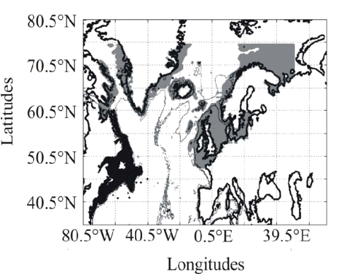
Figure II.2 : Spatial distribution of
observed (Fishbase data, 52,630 datapoints, in black) and inferred (104,642
datapoints, in grey) occurrence data point of the Atlantic cod (Gadus
morhua Linneaus, 1758). Isobaths 200m (dark grey line) and 2000m (light
grey line) are indicated.
? Description of the Non Parametric Probabilistic
Ecological Niche model (NPPEN)
The model is derived from a test recently applied to compare
the ecological niche of two species (Beaugrand & Helaouët 2008). The
analysis is based on Multiple Response Permutation Procedures (MRPP), a test
first proposed by Mielke et al. (Mielke et al. 1981). MRPP has been
applied in conjunction to Split Moving Window Boundary analysis to detect
discontinuities in time series (Cornelius & Reynolds 1991). This method has
also been used to identify abrupt ecosystem shifts (Beaugrand 2004, Beaugrand
& Ibanez 2004). Mathematically, MRPP tests whether two groups of
observations in a multivariate space are significantly separated. (Mielke et
al. 1981) gave a full description of the test and Beaugrand & Helaouët
(Beaugrand & Helaouët 2008) have recently illustrated an adaptation of
the test to compare two ecological niches.
The model we propose to assess the probability of cod
occurrence (and its changes in space and time) is in fact a simplification of
MRPP. Instead of comparing two groups of observations, our new analysis tests
whether one observation belongs to a group of (reference) observations we call
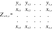
here the reference matrix. The reference matrix is represented by a matrix
Xn,p with n the number of (reference) observations and p the number
of variables. Each row of the matrix represents the environmental conditions
where a species is detected. It is crucial that the reference matrix covers the
entire niche of a species to give a reliable probability (Thuiller 2004); we
check this point, which is often forgotten in this kind of exercise, by
compiling histograms. The predictive matrix Ym,p encompasses m
observations of the environment using p predictors. Each observation of Y,
(environmental conditions) is then tested against X (range of conditions where
the species was detected). The model is applied in 4 main steps:
Step 1: homogenization of the
reference matrix
The density of cod occurrence reported in some databases (e.g.
Fishbase) depends on fishing activities and it is clear that the density of
data points is higher in fishing area. Although this suggests that the resource
is more abundant in those regions, this is not completely true. This phenomenon
can potentially influence the outcome of any ecological niche model. Another
phenomenon that can influence the probability is the inaccurate reporting of
occurrence since misreports can influence the probability. In an attempt to
overcome these drawbacks, we created a virtual cube (i.e. three
controlling factors) with intervals of sea surface temperature of 1°C
between -2°C and 18°C, intervals of bathymetry of 20 m between 0 and
800 m and intervals of annual SSS of 2 between 0 and 40 and retained one data
occurrence when more than one observation were detected in the crossed
intervals of annual SST, bathymetry and annual SSS. This threshold was fixed to
eliminate the impact of one single misreporting. The resolution could, at first
sight, appear to be coarse. However, the practice of the ENM indicates that the
probability remains similar, even at a lower resolution (see Fig. II.4), which
depends on the size of the reference matrix. Here, the size was equal to
140,026 observations. This amount divided by 16,000 (20 SST intervals x 40
bathymetric intervals x 20 SSS intervals) = 8.75 observations per geographical
cell. Such a calculation assumes obviously that observations are equally
distributed, which was clearly not the case. A resolution of 0.1°C for
SST, 1m for bathymetry and 0.1 unit of SSS would appear to be too sensitive as
only 0.02 observations per crossed interval are expected if observations were
randomly distributed. The determination of the threshold also depends on the
uncertainties on the physical variables.
Step 2: preparation of
data
A matrix called Zn+1,p is created for each
observation of Y to be tested against X. For the first observation, the
following matrix is constructed:
 (1) (1)
With xi,j, the observations in matrix
X and yi,j, an observation of matrix
Y. The building of matrix Z is repeated m
times, corresponding to the m observations of Y.
Step 3: calculation of the mean
multivariate distance between the observation to be tested and the reference
matrix
MRPP was first proposed to be applied with an Euclidean
distance, a squared Euclidean distance or a chord distance (Mielke et al.
1981). To first illustrate the technique, we use an Euclidean distance.
Obviously, if variables do not have the same unit or dimension, such a distance
should be avoided. The Euclidean distance is calculated as follows:
 (2) (2)
With z1,j the first observations for the
jth variable originally the observation of the variable of matrix
X, 1 = j = p; zi,j, the observation i of the
variable j in matrix Z with 2 = i = n+1 and 1 = j = p. Then,
the average observed distance åo is calculated as follows:
 (3) (3)
With n, the total number of Euclidean distances, equal to the
number of observations in the training set X.
Step 4: calculation of the
probability that the observation belongs to the reference matrix
The mean
Euclidean distance is tested by replacing each observation of
X by y in Z from row 2 to n+1. The number of
maximum permutations is equal to n. After each permutation, the mean Euclidean
distance ås is recalculated, with 1 = s = n. A probability p
can be assessed by looking at the number of times a simulated mean Euclidean
distance is found to be superior or equal to the observed mean Euclidean
distance between the observation and the reference matrix X.
 (4) (4)
Where the probability p is the number of times the simulated
mean Euclidean distance was found superior or equal to the observed mean
distance. When p = 1, the observation has environmental conditions that
represent the centre of the species niche. When p = 0, the observation has
environmental conditions outside the species niche. It is essential to remind
here that the niche and its borders have to be correctly assessed. Applying the
procedure to each observation of Ym,p leads to a
matrix Pm,1 of probability. It is important to have
a large reference matrix so that the resolution of the probability is as high
as possible. The resolution R of the probability is:
 (5) (5)
With n the number of reference observations in
X. Ideally, R should be < 0.05.
? Simple example of application of the model using the
Euclidean distance
To illustrate the principle of the technique, we present a
hypothetical case where the reference matrix X has n = 3
observations and p = 2 controlling factors while the predictive matrix
Y has m = 1 observation (Fig. II.3). Calculations of the
three Euclidean distances
between y and the reference observations x give  = 2.236, = 2.236,  = 2.236 and = 2.236 and  =1.803 (Fig. II.3a). The average observed distance åo
is = 2.092. The simulated distances are ås1 = 1.589 (Fig.
II.3b), ås2 = 1.383 (Fig. II.3c) and ås3 =
1.140 (Fig. II.3d). The =1.803 (Fig. II.3a). The average observed distance åo
is = 2.092. The simulated distances are ås1 = 1.589 (Fig.
II.3b), ås2 = 1.383 (Fig. II.3c) and ås3 =
1.140 (Fig. II.3d). The
probability is therefore equal to 0. Observation y has
environmental conditions not compatible with the species ecological niche
inferred here from 2 variables.
? Selection of a better coefficient of distance for
Step 2
Mielke et al. (Mielke et al. 1981) used mainly the Euclidean,
squared Euclidean and chord distances. However, in the context of habitat
modelling, the use of the Euclidean (squared or not) distance in step 2 is
inappropriate in most (if not all) cases and the chord distance is often a
better approach (Beaugrand & Helaouët 2008). The computation of the
chord distance is achieved by normalizing each vector of Z to one prior to the
calculation of the Euclidean distances; this is a special kind of scaling
(Legendre & Legendre 1998). Each element of the vector is divided by its
length, using the Pythagorean formula to ensure that each variable carries the
same weight in the analysis. In our study, the normalization of elements of
Zn+1,p (see (1)) would be:
 (6) (6)
Where x and y are as in (1). Here however, we prefer the use
of the Mahalanobis generalised distance that is independent of the scales of
the descriptors (as is the chord distance) but also takes into consideration
the covariance (or the correlation) among descriptors (Ibañez 1981).
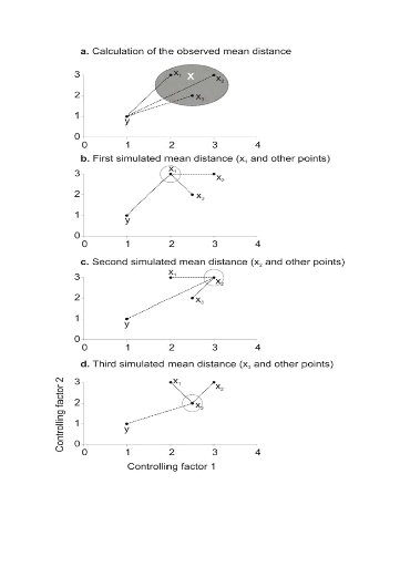
Figure II.3 : Principles of the calculation
of the niche model that lead to probability of occurrence of a species.
A. Hypothetical observations to be tested against a training
set (X) composed of three observations in the space of two controlling factors.
Three Euclidean distances are first calculated and then the average observed
distance between the observation to be tested and the ones of the training set
is assessed. B. Recalculation of the mean distance after
permutation of the first observation (x1) of the training set by the
observation to be tested. C. Recalculation of the mean
distance after permutation of the second (x2) observation of the training set
by the observation to be tested. D. Recalculation of the mean
distance after permutation of the last observation (x3) of the training set X
by the observation to be tested. All calculated Euclidean distances are
indicated by a dashed line. The number of times the simulated mean distance is
found inferior to the observed mean distance defined the probability to find
the species in a region.
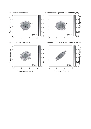
Figure II.4 : Fictive examples that show the
better performance of the Mahalanobis generalised distance in comparison to the
chord distance, justifying the choice of the distance coefficient in the
ecological niche model NPPEN. First, the reference matrix is composed of 25
observations with two controlling factors. The correlation between the 2
controlling factors is null (A and B).
A. Probabilities based on the chord distance (r = 0).
B. Probabilities based on the Mahalanobis generalised distance
(r = 0). Second, the reference matrix is composed of 13 observations with 2
parameters. The correlation between the two controlling factors is high (r =
0.82; C and D). C.
Probabilities based on the chord distance (r = 0.82). D.
Probabilities based on the Mahalanobis generalised distance (r = 0.82). Black
circles denote the reference observations (reference matrix). High
probabilities are located at the centre of the reference matrix, denoting the
centre of the ecological niche (sensu Hutchinson) and probabilities
<0.1 are situated outside (white colour).
The Mahalanobis generalised distance has been frequently used
recently in this context (e.g. Chalenge et al. 2008,
Nogués-Bravo et al. 2008). Prior to the calculation of the distance,
standardisation of Z is accomplished by the following
transformation:
 (7) (7)
Where  are observation i of the jth variables in Z, are observation i of the jth variables in Z,  the average value of variable j and the average value of variable j and  the standard deviation of variable j in Z. To calculate the Mahalanobis
generalized distance between each observation of the environment yi
(1 = i = m) and all observations of the training set xj (1 = j = n),
we used a particular form of the generalized distance, giving the distance
between any observation and the centroid of a unique group (Ibañez
1981): the standard deviation of variable j in Z. To calculate the Mahalanobis
generalized distance between each observation of the environment yi
(1 = i = m) and all observations of the training set xj (1 = j = n),
we used a particular form of the generalized distance, giving the distance
between any observation and the centroid of a unique group (Ibañez
1981):
 (8) (8)
With Rp,p the correlation matrix
of the standardized table Z* (mean 0 and variance
1), k1,p is the vector of the differences between
values of the p variables at  of standardized matrix Z* and the mean of standardized matrix Z* and the mean  of the p variables in the standardized matrix Z*. Therefore
in Step 3, the Euclidean distance was replaced by the use of the Mahalanobis
generalised distance. of the p variables in the standardized matrix Z*. Therefore
in Step 3, the Euclidean distance was replaced by the use of the Mahalanobis
generalised distance.
? Analyses
Analysis 1
A comparison of the model based on a chord distance and the
Mahalanobis generalised distance was performed using an example of 2 variables
and in two cases: no correlation between the two variables (r=0, a training set
of 25 observations) and a strong correlation between the two variables (r=0.82,
a training set of 13 observations) (Fig. II.4).
Analysis 2
The procedure of homogenization was illustrated by compiling
histograms of each predictive variable (annual SST, annual SSS, bathymetry) for
all geographical cells of the spatial domain covered by this study and for both
the original and corrected training (or reference) set (Fig. II.5).
Analysis 3
The model was then applied to project the spatial distribution
of occurrence of Atlantic cod to enable the characterization of its ecological
niche (realized niche) as a function of annual SST, annual SSS and bathymetry
(Fig. II.6). The ecological niche was then projected in the spatial domain as a
combined function of the three environmental parameters (observed annual SST,
annual SSS and bathymetry) for the 1960s, the 1990s and the period 2000-2005
(Fig. II.7). Some projections of changes in the spatial distribution of cod
occurrence, based on modelled SST (scenario A2 and B2; annual SSS and
bathymetry), were provided for the 1990s (for comparison purpose), the 2050s
and the 2090s (Fig. II.8).
2.4. Results
? Analysis 1
A simple example of a training set composed of two variables
(correlated or not) illustrated well the difference between the chord and the
Mahalanobis generalised distances (Fig. II.4). When the correlation between two
parameters was not different to 0, the ecological niche model based on the
chord distance and the Mahalanobis generalised distance gave similar results
(Fig. II.4a-b). However, when the variables of the training set were highly
correlated, the model gave improved results when it was based on the Mahalanobis generalized distance
(Fig. II.4c-d). This fictional example shows shows that the chord distance
should not be used when ecogeographical variables are correlated. Therefore, we
did not calculate the probability of cod occurrence based on this distance.
? Analysis 2
Cod individuals were mainly reported over neritic regions
(Fig. II.5; see also Fig. II.2). Most of the reported cod occurrences (79.87% in the original reference
matrix) were in regions shallower than 200 m and the frequency of cod
occurrence increased when the region became shallower; the homogenisation
procedure did not alter radically the shape of the distribution (Fig. II.5).
Only a fraction of the total records (6.41% of reported cod occurrence) were
deeper than 800 m, the threshold of bathymetry selected in this study. The
sharpness of the continental slope may explain this small percentage since it
is likely that the species can make short incursions over the shelf-edge (small
mistakes on the spatial coordinates could increase this percentage slightly).
Cod are rarely seen in oceanic regions and some authors have proposed a limit
of 600 m, which corresponded to 12.48% of the records (Sundby 2000). To be more
conservative, the bathymetric threshold was increased to 800m.
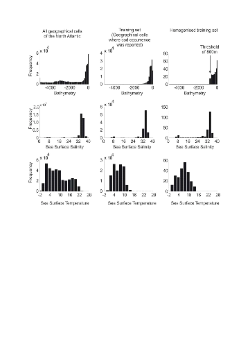
Figure II.5 : Frequency distribution of
bathymetry (upper panels), sea surface salinity (middle panels) and sea surface
temperature (lower panels) in the North Atlantic (from 80.5°W to
70.5°E and from 35.5°N to 70.5°N; left panels), in the original
reference matrix (i.e. geographical pixels where cod occurrence was detected)
and in the homogenised reference matrix (see methods).
The frequency of occurrence showed a mode over 34 for annual
SSS, a mode that corresponds to the one identified when all regions of the
Atlantic were gathered together. Another smaller mode, more visible after
homogenisation, appeared around 8 (Fig. II.5). This mode corresponds to the
salinity observed in the Baltic Sea. While annual SSTs in the regions of the
North Atlantic vary between -2°C and 22°C, with a mode around
2°C, the range of temperature in which cod occurrences were more
frequently reported were over 8°C but range between 2°C and 14°C
in the homogenised reference matrix. The procedure of homogenisation (Step 1)
made it clear that the thermal optimum of the species is about 8°C.
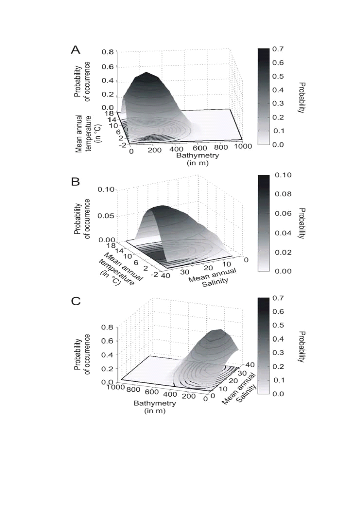
Figure II.6 : Realised niche (sensu
Hutchinson) of the Atlantic cod. A. Probability of cod
occurrence as a function of bathymetry and mean annual sea surface temperature.
B. Probability of cod occurrence as a function of mean annual
sea surface salinity and mean annual sea surface temperature.
C. Probability of cod occurrence as a function of mean annual
sea surface salinity and bathymetry.
? Analysis 3
The model NPPEN was first applied to reproduce the ecological
niche of Atlantic cod as a function of annual SST (observed data), annual SSS
and bathymetry (Fig. II.6). The niche exhibited high probabilities of
occurrence at a bathymetry that ranged between 0 and 500 m (mode between 100 m
and 300 m), an annual SST between -1°C and 14°C (mode between
4°C and 8°C) and an annual SSS ranging between 0 and 36 (mode between
25 and 34) (Fig. II.6).
When projected on the geographical space (Fig. II.7), the
modelled spatial distribution of the probability of cod occurrence was
congruent with the main location of the cod stocks in the North Atlantic sector
(Sundby 2000, Bigg et al. 2008). However, there was a notable exception in the
Baltic Sea where low probabilities of cod occurrence were detected
(Fig. II.7A). A significant decrease in the probability of cod occurrence
was evident between the 1960s and the period 2000-2005 in the North Sea, while
no such a change was visible on the western side of the Atlantic at the
southern range of the spatial distribution of the species. At the northern edge
of the spatial distribution of the species, probabilities of cod occurrence
increased along Greenland and especially in the western regions of this country
and in the Barents Sea. Probabilities around the Faeroes and Iceland remained
stable.
Probabilities of cod occurrence based on modelled annual SST
(ECHAM 4, scenario B2) and observed annual SST were similar (r=0.95,
p<0.01). However, some discrepancies were noted on the western side of the
Atlantic (Fig. II.8D; see (Beaugrand et al. 2008). Based on modelled data, the
probabilities of cod occurrence appear much lower than observed data during the
1990s on the Georges Bank, the Eastern Scotian Shelf and the Grand Bank
(Fig. II.8D).
The examination of long-term decadal changes in the
probability of cod occurrence projected for this century suggests a clear
northward movement of this species (Fig. II.9). Interestingly, the probability
of cod occurrence decreased substantially at the southern edge of the range of
the species: the North Sea, Georges Bank, Eastern Scotian Shelf, Grand Bank and
Newfoundland. The probabilities increased in the Barents Sea and in areas close
to Greenland while no major changes were detected for Iceland. A substantial
decrease in the probability of cod occurrence is also suggested by the model
around the Faeroes at the end of this century if long-term changes in SST
follow Scenario B2 (Fig. II.9D).
Figure II.7 : Modelled spatial
distribution in the probability of cod occurrence. A.
Probability of cod occurrence for the period 1960-1969. B.
Probability of cod occurrence for the period 2000-2005.
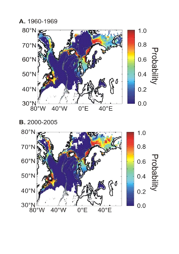
Figure II.8 : Modelled spatial
distribution in the probability of cod occurrence for the period 1990-1999.
A. From modelled annual SST (ECHAM 4, scenario B2).
B. From observed annual SST. C. Relationships
between probabilities based on observed and modelled (ECHAM 4, scenario B2)
annual SST. The Pearson coefficient of correlation is indicated. Probabilities
assessed from Scenario A2 gave similar conclusions. D.
Difference between probability of cod occurrence based on modelled SST (A) and
probability of occurrence based on observed SST (B).
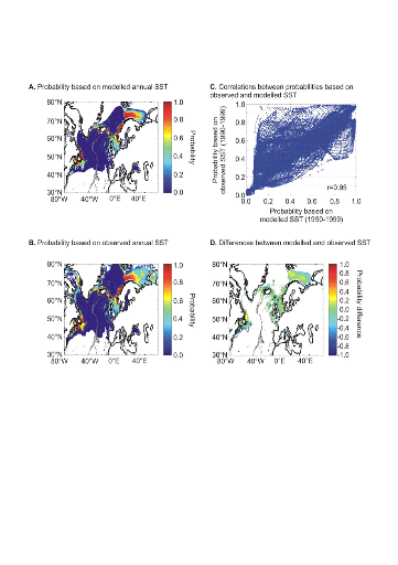
The probability of cod occurrence was sensitive to the
intensity of warming (Fig. II.10). This sensitivity was not constant in
space. Major changes occurred in areas located at the southern or northern
limit of the spatial distribution of the species. When the level of
anthropogenic warming remained unchanged (Fig. II.10A-B), the probability of
cod occurrence remained high in regions located at the southern limit (or low
at the northern limit) of the spatial distribution of the species. However,
even with a moderate scenario (Scenario B1, Fig. II.10C), the probability of
cod occurrence decreased in key regions such as the North Sea and the Georges
Banks. When the level of anthropogenic warming increased, this had a pronounced
influence in regions such as the North Sea and the Eastern Scotian Shelf
(Fig. II.10D-E).
The coefficient of variation calculated per geographical cell
using all 7 simulations issued from the three models (ECHAM4, HadCM3, HadGEM1)
showed the areas where the changes are expected to be the most prominent (Fig.
II.10F). This analysis showed that modifications are expected to be pronounced
at the periphery of the current spatial distribution of species. High values
were observed in the Barents Sea where a strong increase in the probability of
cod occurrence is expected in the case of an intense warming and to a lesser
extent in areas such as the North Sea and the Georges Bank.
Figure II.9 : Projected long-term
decadal changes in the probability of cod occurrence from modelled annual SST
(Scenario B2). A. Period 1990-1999. B. Period
2050-2059. C. Period 2090-2099. Probabilities assessed from
Scenario A2 gave similar conclusions. D. Difference of
modelled probability of occurrence between periods 2090-2099 and 1990-1999.
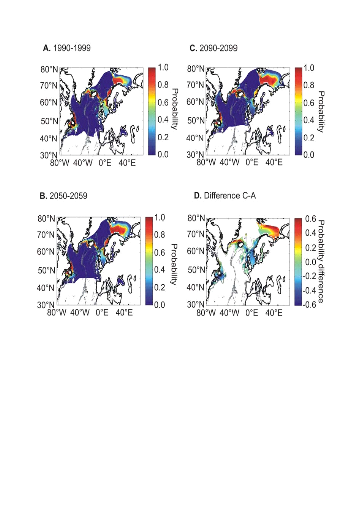
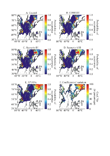
Figure II.10 : Projected long-term decadal
changes in the probability of cod occurrence for the period 2090-2099.
A. scenario `Control'. B. Scenario COMMIT.
C. SRES scenario B1. D. SRES scenario A1B.
E. 1PTO4x. F. Coefficient of variation (Coef.
Var) based on the 7 scenarios and 3 atmosphere-ocean general circulation models
(see methods). The intensity of warming increases from A to E.
2.5. Discussion
To predict how the spatial distribution of marine species may
change with climate, it is essential to understand the factors that limit their
distributions. One way to achieve this is to use ecological niche models.
However, only a limited number of models can deal with presence-only data. The
models BIOCLIM and HABITAT use a rectilinear volume and a convex envelope
(i.e. a closed polygonal chain), respectively (Carpenter et al. 1993).
The drawbacks to these simple models are the imposed shapes, which can be the
cause of a non-justified exclusion or inclusion of a geographical point from
the predicted distribution (Carpenter et al. 1993). The model DOMAIN can solve
this problem by the use of a point-to-point similarity metric. However, the
metrics used (e.g. the Gower metric; Carpenter et al. 1993, Legendre
& Legendre 1998) does not take into account the correlation between
descriptors (Legendre & Legendre, 1998). Furthermore, a threshold is used
to map the modelled distribution of the species. The RES model (Kaschner et al.
2006) uses a trapezoid shape that constitutes a good compromise between species
with a shorter or a unimodal ecological niche and migratory species with larger
or a bimodal niche (Kaschner et al. 2006). However, the bounds of this
trapezoid need to be precisely defined, implicating often arbitrary choices and
thus it requires a good knowledge of the species. While the Ecological Niche
Factor Analysis (ENFA; Hirzel et al. 2002) could be adapted for our study, this
technique requires the multinormality of the ecogeographical variables to
extract the eigenvectors to calculate the marginality and the specialization
factors and thereby a transformation of the ecogeographical variables is often
needed (e.g. Box-Cox) prior to the analysis. Finally, the statistical technique
MAXENT (Philips et al. 2006), which is based on the maximum-entropy principle,
also requires accurate threshold definition and showed some application
restrictions.
NPPEN offers a number of advantages on the above existing
methods. Firstly, contrary to models such as RES (Kaschner et al. 2006) or the
mixed model of Cheung and colleagues (Cheung et al. 2008a), our simple model
does not need an a priori knowledge of the species biology. Our
technique is also based on a non-parametric test that does not require the
multinormality of the ecogeographical variables. Although the use of the
Generalised Mahalanobis distance is not new in this kind of model (Farber &
Kadmon 2003, Cayuela 2004, Etherington et al. 2009), this is the first time
that this distance metric is embedded into a non-parametric test. For example,
Cayuela (Cayuela 2004) rescaled the Mahalanobis distance into quantiles to
produce a map of probability and Nogués-Bravo et al.
(Nogués-Bravo et al. 2008) converted the distance into quartiles.
Ibañez (Ibañez 1981) or Farber & Kadmon (Farber & Kadmon
2003) tested this distance by approximating this measure by a ÷²
distribution with n-1 degrees of freedom. Legendre & Legendre (Legendre
& Legendre 1998) also described the conversion of the D² by the
Hotelling T² (Hotelling 1931) statistic and its test by the F statistic.
These tests require the distribution to be multinormal. Although these authors
stated that the test can tolerate some degrees of deviation from this
assumption, it can be seen from histograms that the bathymetry data (Fig. II.5)
were very far from the normality. Finally, the procedure does not need the
selection of arbitrary thresholds and is fully statistical. The technique
simply tests whether an observation belongs to a group of observations called
here a training set or a reference matrix. NPPEN therefore can be used very
quickly as an exploratory analysis to give a first approximation of the spatial
distribution of a species. The test is also appropriate for many species for
which no information on the physiology exists. The only caveat is that our
model, as others, does not fully resolve the problem of autocorrelation (SAR).
The spatial autocorrelation can inflate significantly the probabilities
inferred from ENMs (Bahn & McGill 2007). We think that presence-only
technique of ENMs are much less subject to this problem than other types of
ENMs (e.g. GLM). The problem is that only few studies considered local
functions of autocorrelation (Beaugrand & Ibañez 2002, Dormann et
al. 2007). Most corrections applied are based on global function of
autocorrelation with underlying assumption of isotropy (e.g. the
Moran' index, global semivariograms), which is rarely the case in
biogeography (Beaugrand & Ibañez 2002).
Our technique is currently restricted to presence-only data.
Although some adjustments could be made to apply the method (e.g.
calculate the test for different category of abundance), it is probably
preferable in such a case to use other techniques such as Generalised Linear
Model (GLM; McCullagh & Nelder 1983) or Generalised Additive Models (GAM;
Hastie & Tibshirani 1990). Guisan & Zimmermann (Guisan & Zimmermann
2000) provided an extended review on the different techniques used to assess
the spatial distribution of a species. Perhaps, another limitation of the
technique lies in the fact that it should only be employed with a limited
number of ecogeographical variables. If a high number of variables are used it
would be preferable to use a principal component analysis prior to the
application of the test, or use the Mahalanobis distance factor analysis
(MEDIFA; (Calenge et al. 2008) to better understand the contribution of the
ecogeographical variables; this can also be done a posteriori by
calculating the correlation (here, the rank correlation coefficient of Spearman
or Kendall (Legendre & Legendre 1998) between the modeled probability and
each environmental factor. NPPEN might also be subjected to what could be
described as a «border effect». Indeed, the modelling of the niche of
Atlantic cod (see Fig. II.6) showed a reduction in the probability of cod
occurrence towards shallow regions, which is unexpected based upon our
knowledge of the species (Sundby 2000). Indeed, the technique works in such a
way that maximum probability is concentrated towards the middle of the niche.
Therefore some borders of the multidimensional niche might be underestimated.
Although this problem is difficult to circumvent, it could be overcome
partially by modelling the absence of the species (i.e. estimate the
probability of the absence of the species). Probabilities issued from such a
modelling approach would be less sensitive to the border effect discussed above
and would be complementary, i.e. by assessing the
fundamental niche whereas the ENMs applied on presence data estimate the
realized niche (Pulliam 2000, Helaouët & Beaugrand 2009).
Modelling the absence of a species has never be done, as far
as we know, however, this could be as interesting as modelling the presence of
a species, especially in the case of an exploited species such as Atlantic cod.
Indeed, modelling the probability of absence is very informative for
policymakers and fisheries scientists. It should not be assessed from map of
probability of presence however, but instead should be based on physiological
evidence (Bigg et al. 2008, Helaouët & Beaugrand 2009). When
presence-only data are available to model the spatial distribution of cod,
several known scientific facts and physiological evidence exist that could be
used in NPPEN. First, the species is generally found where the bathymetry is
shallower than 800 m (see Fig. II.5). While some authors found a sharp decrease
in the frequency of occurrence of this species at 400 m and an absence from 600
m (Bigg et al. 2008), this not a sharp constraint and so we can be
conservative. From field and experimental studies, we know that cod are unable
to reproduce at salinities below 11 because their sperm become immobile and
their eggs sink (Brander, Personal Communication), therefore we can predict
confidently that cod will cease to reproduce in areas where salinity falls
below these levels. For temperature, different thresholds could be used.
Beaugrand et al. (Beaugrand et al. 2008) found a pronounced increase
in the variance of the Atlantic cod when the thermal regime was between 9 and
12°C with maximum variance between 9 and 10°C. Brander (2005) in a
synthesis report on this species found maximum spawning temperatures of
12.7°C in Georges Bank. Pepin et al. (1997) found a sustained decrease in
the percentage of egg survival in laboratory between 10° and 12°C.
Here also, it would be logical to select the threshold of 12.7°C (as
monthly SST) in order to remain conservative.
Our model explains in part the pronounced decrease observed in
the abundance of cod in the North Sea (Brander et al. 2006) although the
decline modelled from our study seems less pronounced. Two main phenomena could
explain this result. First, our model does not incorporate information on
plankton. Recent studies have shown however that plankton amplifies the effect
of temperature change (Beaugrand & Kirby 2010b, a). If plankton exacerbates
the effect of climate, our model could be too conservative. Second, overfishing
has exerted a sustained pressure on the stock that has probably increased its
sensitivity to climate change (Hsieh et al. 2006). It is also expected that
these two phenomena act in synergy to reduce the size of the stock (Kirby &
Beaugrand 2009). Our model only explains in part the collapse of cod observed
in eastern part of North America (e.g. The Georges Bank, the Eastern Scotian
Shelf and Newfoundland). This is mainly observed when our model is based on
modelled SST data (Fig. II.8). Recently, Beaugrand & Kirby (Beaugrand &
Kirby 2010a) also show that some plankton indicators decreased at the same time
than the observed collapse of cod stocks in these regions. However, the region
is complex and some other plankton variables were unable to explain completely
this collapse. Here also, overfishing has had a well-documented effect (Myers
et al. 1996, Hsieh et al. 2006). The stock may resist sustained pressure up to
a point when environmental conditions become less favorable and trigger the
collapse of the stock. While it is impossible to compensate directly for both
the direct and indirect effects of global warming on the ocean, the
consideration of change in the carrying capacity of the ecosystem in the
management of the species should be made more explicit in ecosystem fisheries
based management (Pikitch et al. 2004).
Finally, projections suggest substantial changes in the
spatial distribution of cod at the scale of the North Atlantic Ocean. Our
projections indicate that cod should decrease to the level of commercial
extinction in the North Sea and in regions on the eastern side of North America
(e.g. Georges Bank, the Scotian Shelf and Newfoundland) where collapses have
already been detected. These results tend to suggest that the rebuilding of cod
stocks in the North Sea might be difficult. Instead, our effort should perhaps
be made on what resource is likely to present or to develop over the next
decades to enable fishermen to anticipate changes in the resources should
climate continue to warm.
Acknowledgements
We thank Dr Richard R Kirby for helpful comments on an early
version of the manuscript. We are grateful to past and present members and
supporters of the FishBase website
(http://www.FishBase.org), whose continuous efforts have
allowed the establishment of the fish data set. We thank Dr Keith Brander for
helpful comments on an early version of the manuscript. The research was
supported by the French Agency of Research and Technology (ANRT, grant CIFRE
862/2007).
CHAPITRE III
Distribution spatiale modélisée des
poissons marins et projections des changements dans l'océan Atlantique
Nord
1. Résumé du
chapitre III
1.1. Avant-propos
Les stocks de poissons fluctuent dans le temps et l'espace.
Comprendre pourquoi et comment ces stocks varient, représente un enjeu
majeur pour les politiques de gestion durable des ressources et pour les
professionnels du secteur de la pêche (Rosenzweig, 1995; Barange &
Harris, 2003). De nombreux outils existent pour évaluer et
prédire les changements dans la dynamique des stocks liés
à l'exploitation ou aux processus intraspécifiques, telle la
relation stock-recrutement. En revanche, l'étude de l'impact du climat
et plus particulièrement du réchauffement climatique, n'est
encore que rarement intégrée dans les plans de gestion durable
des ressources marines. La nature systémique de la gestion de ces
ressources est une vision récente (Cury et al., 2008).
Pourtant, de nombreuses études ont mis en évidence les
conséquences multiples du réchauffement climatique sur
l'écosystème marin (Edwards & Richardson, 2004; Brander,
2007; Stempniewicz et al., 2007; Kirby & Beaugrand, 2009). La
redistribution des espèces est l'une de ces conséquences,
régulièrement observée (Beaugrand et al.,
2002 ; Harris et al., 2007). De la même façon,
l'augmentation régionale de l'abondance de certaines espèces est
expliquée par l'augmentation des températures de l'eau dans ces
régions (Kirby et al., 2006; Van Damme & Couperus, 2008).
Les poissons marins exploités connaissent également ces
changements (Quero et al., 1998; Brander, 2003 ; Drinkwater 2005;
Perry et al., 2005).
L'objectif de cette étude était de mettre en
lumière l'impact prépondérant du climat et du
réchauffement climatique sur la distribution spatiale de huit
espèces de poissons. Pour ce faire, la niche écologique des
espèces a été retracée à partir de leurs
préférendums, eux-mêmes évalués uniquement
à partir de données de présence des espèces. Le
modèle NPPEN a été utilisé pour cartographier la
répartition géographique passée, présente et
potentielle de ces poissons, en fonction de trois paramètres
environnementaux (SST, bathymétrie et SSS). Le modèle NPPEN a pu
ainsi être testé sur différents types de jeux de
données (complet ou incomplet, homogène ou non...). La robustesse
des résultats a été estimée par comparaison avec
ceux d'un autre modèle : le modèle Relative Environmental
Suitability (RES, Kaschner et al., 2006). Au final, des cartes
illustrant les pertes et gains possibles pour chacun des poissons ont
été produites.
1.2. Données
utilisées
? Données biotiques
Huit espèces de poissons ont été choisies
pour leur importance commerciale, et en fonction de leurs
préférences bathymétriques (espèces
pélagiques, démersales ou benthiques) et thermiques
(espèces d'eaux tempérées, tempérées-chaudes
ou tempérées-froides) :
(1) le chinchard de l'Atlantique (Trachurus trachurus
Linnaeus, 1758),
(2) l'anchois européen (Engraulis encrasicolus
Linnaeus, 1758),
(3) le sprat européen (Sprattus sprattus
Linnaeus, 1758),
(4) le lieu jaune (Pollachius pollachius Linnaeus,
1758),
(5) la sole commune (Solea solea Linnaeus, 1758)
(6) l'églefin (Melanogrammus aeglefinus
Linnaeus, 1758)
(7) le lieu noir (Pollachius virens Linnaeus,
1758),
(8) le turbot (Psetta maxima Linnaeus, 1758).
Les données de présence de ces espèces
ont été récupérées, comme mentionné
dans le chapitre II, à partir de la base de données en ligne
FishBase (Froese & Pauly, 2009), complétée avec des
données provenant du Conseil International pour l'Exploitation de la Mer
(CIEM, 2005b, 2007), de la littérature et des connaissances
scientifiques sur la distribution spatiale de ces espèces. Ces
observations sont datées et géo-référencées.
? Données abiotiques
Comme dans le chapitre II, les jeux de données des
trois paramètres physiques considérés ont
été compilés : la température de surface (SST)
de 1960 à 2005, la bathymétrie, la salinité de surface
(SSS).
Seuls les scénarios d'évolution du climat SRES
A2 et B2 du modèle ECHAM4 ont été inclus pour
modéliser la distribution potentielle future des espèces.
La zone géographique couverte par les trois variables
s'étend des latitudes 25°N à 85°N et des longitudes
80°W à 65°E (Fig. III.1). Suivant la même
procédure que dans le IIe chapitre, les valeurs des trois
variables sont interpolées de façon bilinéaire avec une
résolution 0,1° de latitude et de longitude, pour créer un
jeu de cartes environnementales similaires : une carte de
bathymétrie, une carte de SST et une carte de SSS, par année, de
1960 à 2100.
1.3. Méthode et
Analyses effectuées
? Méthodes
Le NPPEN, décrit dans le chapitre II, a
été utilisé.
? Analyse 1
À partir des données brutes d'observation et
d'homogénéisation, les préférendums des huit
espèces ont été évalués pour chacun des
paramètres (Fig. III.2 et Fig. III.S9).
? Analyse 2
Une évaluation des capacités du modèle
à reconstruire la niche écologique d'une espèce a
été menée. Un cas idéal de référence
(R) a été défini à partir de données
d'observations de l'espèce, couvrant de façon homogène
chaque gradient environnemental (Fig. III.3a). Ce cas idéal (R) est
comparé à des cas simulés (S) pour lesquels les
données d'observation de l'espèce se répartissent le long
des gradients environnementaux de façon : proche de
l'homogénéité (Fig. III.3b), bimodale symétrique
(Fig. III.3c) et bimodale asymétrique (Fig. III.3d). Les
différences moyennes entre les différents cas (S) et le cas de
référence (R) sont calculées.
? Analyse 3
Le NPPEN a été appliqué pour
modéliser la niche écologique des huit espèces de poissons
considérées dans l'étude. Puis, ces niches
écologiques ont été projetées dans l'espace
environnemental (SST, bathymétrie, SSS) pour différentes
périodes : 1960-1969, 2000-2005, 2050-2059, 2090-2099 (Fig.
III.5).
? Analyse 4
Les résultats de la modélisation de la
distribution spatiale des huit espèces par le NPPEN ont
été comparés, par corrélation, à ceux
obtenus avec le modèle Relative Environmental Suitability (RES ;
Kaschner et al., 2006). Cette comparaison a été
réalisée pour la période 1960-2005. Le degré de
liberté requis pour avoir une corrélation significative (p=0,05)
a été calculé afin d'évaluer l'impact de
l'autocorrélation lorsque les cartes de distribution des deux
modèles sont comparées (Table III.1 ; Beaugrand &
Helaouët, 2008).
? Analyse 5
Les probabilités de présence (p) des huit
espèces de poissons ont été converties en données
binaires (si p=0,2 alors p devient p=1; si p<0,2 alors p devient p=0) pour
construire des cartes de distribution de
« présence » modélisée par
période. Les différences entre ces cartes des périodes
2000-2005 et 1960-1969 puis des périodes 2090-2099 et 1960-1969 ont
été calculées. La surface des aires géographiques,
pour lesquelles ces différences n'étaient pas égales
à 0, a été assimilée à un trapèze et
a été estimée dans le but d'évaluer les zones
géographiques potentiellement « perdues » ou
« gagnées » par chacune des espèces (Fig.
III.6, Table III.2).
1.4. Principaux
résultats obtenus
? Analyse 1
L'étude des préférendums thermiques a
confirmé les contraintes et exigences environnementales
différentes pour les espèces étudiées. Ce
résultat permet de souligner l'importance de chacun des descripteurs
environnementaux pour la distribution spatiale des poissons marins.
? Analyse 2
Le modèle NPPEN semble, malgré un nombre
réduit ou un manque d'homogénéité des
données d'observations, capable de retranscrire de façon proche
de la réalité, la niche écologique des espèces. Les
limites de distribution des données, le long des gradients
environnementaux, paraissent jouer un rôle plus important que le nombre
et l'homogénéité de ces données.
? Analyse 3
Les cartes de distribution obtenues coïncident avec les
distributions connues réelles pour les huit espèces
considérées. Trois types de répartitions
géographiques sont retrouvés : (1) la mer du Nord et la mer
Celtique (sprat européen, turbot et lieu jaune); (2) le sud de la mer du
Nord, la Manche et la façade Atlantique de l'Europe (anchois
européen, sole commune et chinchard de l'Atlantique) et (3) du sud de la
mer du Nord au nord la mer de Barents (lieu noir et églefin).
? Analyse 4
L'étude de la corrélation, entre les
résultats issus du modèle NPPEN et ceux du modèle RES,
montre que ces deux techniques, différentes dans leur
interprétation de la forme de la niche écologique (forme
trapézoïdale et forme Gaussienne), produisent des résultats
équivalents en termes de réalisme.
? Analyses 5 et 6
Selon le modèle, toutes les espèces
étudiées semblent poussées vers des latitudes
supérieures par le réchauffement des eaux. Si certaines de ces
espèces paraissent pouvoir s'établir durablement à ces
nouvelles latitudes, d'autres comme le lieu jaune pourraient ne pas trouver des
conditions environnementales en rapport avec leurs exigences. Au final, le
bilan des changements de répartition attendus révèle que
les espèces à niche écologique plus étroite
risqueront d'avoir le bilan le plus négatif.
1.5. Conclusion
Le modèle NPPEN confirme, dans ce chapitre, sa
capacité à prédire la distribution spatiale des poissons
marins à l'échelle de l'Atlantique Nord, et ce à partir
uniquement de données de présence. Contrairement au RES, le NPPEN
à l'avantage de ne pas considérer la niche comme ayant une forme
trapézoïdale mais comme suivant une forme théorique
Gaussienne, plus en rapport avec la définition donnée par
Hutchison (Hutchinson, 1957). De plus, même si la pertinence des
résultats augmente avec le nombre de données de présence,
un nombre plus restreint de données peut suffire à produire de
bons résultats, dès lors qu'il permet de bien délimiter
les contours de la niche écologique des espèces.
La cartographie de la répartition spatiale potentielle
des huit espèces de poissons étudiées montre que, dans un
océan plus chaud, une tendance générale de
déplacement de ces populations de poissons vers des latitudes
supérieures, est attendue. La vitesse et l'intensité de ce
déplacement seront fonction, d'une part, de la vitesse et de
l'intensité du réchauffement climatique ; et d'autre part de
la possibilité qu'auront les espèces à trouver des
enveloppes environnementales en adéquation avec leur niche
écologique. Ainsi, certaines espèces à la niche
écologique plus étroite, tel le lieu jaune, risquent de se
raréfier dans le futur.
2. Publication: Modelled
spatial distribution of marine fish and projected modifications in the North
Atlantic Ocean
Modelled spatial distribution of marine fish and
projected modifications in the North Atlantic Ocean
Running head: Niche modelling and fish
biogeography
S. Lenoir, G. Beaugrand, É. Lécuyer
Global Change Biology 17(1) 2010
2.1. Abstract
The objectives of this work were to examine the past, current
and potential influence of global climate change on the spatial distribution of
some commercially exploited fish and to evaluate a recently proposed new
Ecological Niche Model (ENM) called
Non-Parametric Probabilistic
Ecological Niche model (NPPEN). This new
technique is based on a modified version of the test called Multiple Response
Permutation Procedure (MRPP) using the generalized Mahalanobis distance. The
technique was applied in the extratropical regions of the North Atlantic Ocean
on 8 commercially exploited fish species using three environmental parameters
(sea surface temperature, bathymetry and sea surface salinity). The numerical
procedure and the model allowed a better characterisation of the niche
(sensu Hutchinson) and an improved modelling of the spatial
distribution of the species. Furthermore, the technique appeared to be robust
to incomplete or bimodal training sets. Despite some potential limitations
related to the choice of the climatic scenario (A2 and B2), the type of
physical model (ECHAM 4) and the absence of consideration of biotic
interactions, modelled changes in species distribution explained some current
observed shifts in dominance that occurred in the North Atlantic sector, and
particularly in the North Sea. Although projected changes suggest a poleward
movement of species, our results indicate that some species may not be able to
track their climatic envelop and that climate change may have a prominent
influence on fish distribution during this century. The phenomenon is likely to
trigger locally major changes in the dominance of species with likely
implications for socio-economical systems. In this way, ENMs might provide a
new management tool against which changes in the resource might be better
anticipated.
Keywords: ecological niche modelling, climate
change, marine fish distribution, ecological niche, projections,
biogeography
2.2. Introduction
Fish stocks fluctuate in space and time and the better
understanding of these fluctuations have occupied scientists for several
decades (Rosenzweig 1995; Barange & Harris 2003; Brander 2007). While it
has been difficult to identify causes for some stock fluctuations, changes have
often been attributed to stochastic events (Hsieh et al. 2005),
hydro-climatic anomalies (Edwards et al. 2002; Lehodey et al.
2006), climate change (Drinkwater 2006; Brander 2007) or both direct and
indirect anthropogenic impacts (Hutchings 2000; Jennings et al. 2001;
Pauly et al. 2005). Among anthropogenic pressures, overfishing is an
important driver of change in marine fish stocks, acting probably in synergy
with climate forcing (Hsieh et al. 2006; Brander 2007).
The impact of climate warming on marine ecosystems has become
prominent (Root et al. 2003; Intergovernmental Panel on Climate Change
2007b; Rosenzweig et al. 2008). Among these effects, there is a
central and growing concern about possible changes in species geographical
distribution (Parmesan & Yohe 2003; Deutsch et al. 2008;
Thuiller et al. 2008). For example, northward movements in calanoid
copepod zooplankton have been observed in the North Atlantic Ocean at a mean
rate of up to 23.16 km.y-1 for some species assemblages in a
period of 48 years (Beaugrand et al. 2009). These changes in plankton
composition were paralleled by a northward migration of both commercial and
un-commercial fish species (e.g. Quero et al. 1998; Stebbing et
al. 2002; Brander et al. 2003; Beare et al. 2004a;
Perry et al. 2005).
Despite the recognition of the importance of ecosystem
processes to better manage fish stocks (e.g. Ecosystem Based Fisheries
Management; see Cury et al. 2008), current management plans rarely
consider that the carrying capacity of the ecosystem may fluctuate and that the
natural spatial distribution of the target species may vary. The biosphere is
now experiencing a period of rapid and sustained climate change that might even
accelerate in the future (Intergovernmental Panel on Climate Change 2007b). A
fundamental challenge for future sustainable exploitation and conservation is
to dispose of valid estimations of potential changes in future species
distributions (Pearson & Dawson 2003; Schwartz et al. 2006;
Thuiller 2007). To do so, an increasing number of statistical tools (e.g.
bioclimatic envelop models, ecological niche modelling; Guisan & Zimmermann
2000; Thuiller 2003; Austin 2007) have been developed to determine the
potential response of species to global warming in both the terrestrial
(Harrison et al. 2006; Murphy & Breed 2007; Huntley et
al. 2008) and the marine realms (Guinotte et al. 2006; Beaugrand
& Helaouët 2008; Cheung et al. 2008a). Based on the
Hutchinsonian concept and the relation between species niche and distribution
(Hutchinson 1957; Pulliam 2000), these models project the multidimensional
distribution of species into an environmental (or Euclidean) space or into a
geographical space (Soberón & Peterson 2005; Austin et al.
2006; Hirzel et al. 2006).
The aim of this work is to formulate different scenarios of
changes in the spatial distribution of some North Atlantic fish in response to
ocean warming. First, the ecological niche (sensu Hutchinson, 1957) of
eight exploited fish in the North Atlantic is characterised. Second, the
spatial distribution of these species is modelled for the period 1960-1969.
Third, an evaluation of the consequences of changes in temperature on spatial
distribution of species is carried out during the period 1960-2005. Fourth,
scenarios of changes in the spatial distribution of these species are proposed
for the middle and the end of this century using two moderate scenarios (A2 and
B2). Results are commented in the context of global climate change and
associated to the pronounced influence of fishing on exploited resources and
marine ecosystems.
2.3. Materials and
Methods
? Biological Data
Eight species were chosen according to their economic
importance, their scientific interest and perhaps more importantly the
information available for each of them. Each selected species had a minimum of
a least 813 records (Supplementary Table III.1). Some were pelagic, demersal or
benthic. Species chosen were (Supplementary Table III.1) (a) Atlantic horse
mackerel, (b) European anchovy, (c) European sprat, (d) pollack, (e) common
sole, (f) haddock, (g) saithe, and (h) turbot. The Atlantic cod (Gadus
morhua L.) was not investigated in this paper as it has been recently
described in detail in Beaugrand et al. (submitted) using the same
statistical approach and in Bigg et al. (2008) using the model MAXENT
(Phillips et al. 2006). Current information on the spatial
distribution of these species is presented by Fig. III.S1. They came from two
sources: The Food and Agriculture Organization of the United Nations (FAO;
http://www.fao.org/fi/figis/maps/compilat.htm)
and FishBase (Froese & Pauly 2009;
http://www.FishBase.org). More
information on the spatial and temporal coverage of the datapoints can be found
for each species in Supporting Information (Figs. III.S2 to III.S9).
Biological data were uniquely composed of occurrence data
(Fig. III.1(a)). These data came from three difference sources: (1) FishBase
(Froese & Pauly 2009) using data from the Ocean Biogeographic Information
System (OBIS;
http://www.iobis.org); (2)
ICES-FishMap online atlas (
http://www.ices.dk/marineworld/fishmap/ices/);
(3) experts' knowledge. Each occurrence was spatially located (as longitude and
latitude) and most of them had information on year. No distinction was made
between fish sex and age, and observations retained for the analyses always
resulted from catch of post-larval stages and occurrence data taken from 1960
onwards.
? Environmental data
A set of environmental data was selected to model the spatial
distribution of fish.
Annual Sea Surface temperature
Annual Sea Surface Temperatures (SST) were chosen because this
parameter has strong impacts on a large range of biological processes and on
the spatial distribution of marine fish (Tåning 1948; Crisp 1959;
Pörtner et al. 2001). This parameter remains relevant for benthic
or demersal fish because these species still have a pelagic stage in the life
cycle. This larval stage is a critical life cycle phase affecting recruitment
(see Cushing 1996). Many studies have shown that the environment exerts its
major influence on fish through the effects of temperature on larval
development and plankton food availability (e.g. Beaugrand et al.
2003; Drinkwater et al. 2010). Correlation between SST and
temperatures at 100 m (data from the World Ocean Atlas 2005; Antonov et
al. 2005) was equal to 0.96. The intercept identified by linear regression
indicates that we have to subtract 1.85°C from the SST value to achieve
the 100 m temperature at the scale of our study. Therefore, at the scale of our
study, consideration of temperature at 100m or deeper would not radically
affect our conclusions. Observed annual SST from 1960 to 2005 used in this
study came from the database International Comprehensive Ocean-Atmosphere Data
Set (ICOADS,
http://icoads.noaa.gov;
Woodruff et al. 1987; Fig. III.1(b)). Forecasted annual SST originated
from the ECHAM 4 model (EC for European Centre and HAM for Hamburg;
Roeckner et al. 1996). The present data were chosen by the IPCC on the
basis of criteria among which are physical plausibility and consistency with
global projections. Data utilised here are modelled data based on scenario A2
and B2 (Intergovernmental Panel on Climate Change, 2007b). These data were
averaged for two decadal periods: 2050-2059 and 2090-2099.
Bathymetry
Bathymetry was selected as this parameter strongly influences
the potential habitat of marine fish (Louisy 2002). This factor is frequently
integrated in ENMs (Hedger et al. 2004; Kaschner et al.
2006). Bathymetric data originated from the global ocean bathymetry map
(1° longitude ×1° latitude). The map was constructed from data
obtained from ships with detailed gravity anomaly information provided by the
satellite GEOSAT and ERS-1 (Smith & Sandwell 1997; Fig. III.1(c)).
Figure III.1 : Spatial distribution of
both biotic and abiotic data. (a) Spatial distribution of
occurrence points for the eight species selected in the study. Points of fish
occurrence were reported in blue dots for FishBase (FB), red dots for ICES
(ICES) and cyan dots for other sources (OD); each dot represents the occurrence
of fish post-larval stages without sex distinction; (b)
spatial distribution in the mean sea surface temperature (1960-2005);
(c) spatial distribution in the bathymetry;
(d) spatial distribution in the annual sea surface salinity
(climatology).
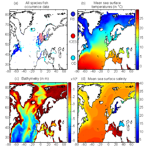
Average Sea surface salinity
Capacity of dispersal can be modulated by Sea Surface Salinity
through the ability of fish to osmoregulate (Schmidt-Nielsen 1990). Annual Sea
Surface Salinity (SSS, average values between 0 and 10 meters, Fig. III.1(d))
data were obtained from the Levitus' climatology (Levitus 1982). ICES data (
http://www.ices.dk) were used to
complete the Levitus' dataset in coastal regions where there is no assessment
of annual SSS (e.g. some regions of the eastern English Channel).
? Statistical procedures
Step 1: interpolation of
environmental data
Both observed and projected annual SST, bathymetry and annual
SSS were interpolated linearly on a 0.1°×0.1° spatial grid to
fit more closely the coasts on the maps. The spatial domain ranged from
110°W to 70.5°E and from 50°S to 90°N. However, only the
part of the North Atlantic ranging from 80°W to 70.5°E and from
25°N to 85°N was investigated for fish spatial projections. This
represented a total of 2,530,206 geographical cells.
Step 2: attribution of
environmental parameters at each fish occurrence point
The environmental stratum (i.e. the combination of three
environmental parameters or triplet; Guisan & Zimmermann 2000) for each
occurrence point and each fish were recovered from the environmental datasets.
When the date of an observation was unknown, an average was used for the time
period 1960-2005 to attribute a mean environmental combination at the
geographical location. This average is unlikely to affect strongly the thermal
niche of the species, which is much more influenced by the spatial than the
temporal variance in SST (Beaugrand et al. 2008). In the same way,
when the date of trawl or observation was available in the form of a time
period (e.g. catch data from 1985 to 1995), the environmental stratum was
averaged for this time period. This pre-processing of the data led to eight
matrices (we called training sets or reference matrices Zn,p), one
matrix per species, each having n observations with three environmental
parameters (see Supplementary Table III.1 for the values of n for each
species; p=3).
Step 3: corrected training
set
The ENM uses the above matrices to evaluate the probability of
occurrence of each species. However, as they stand, the reference matrices
could be biased towards regions more investigated than others due to
concentration of fishing activities or scientific campaigns. To consider this
potential drawback, the reference matrices were corrected prior to the
application of the model. This procedure was similar to what is performed in
the programme RASTERIZ included in the GARP Modelling System (GMS; Stockwell
& Peters 1999) and was implemented to give the same weight to regions of
small or massive occurrence densities. A three-dimensional matrix was defined.
The first dimension, reflecting SST, varied between 0°C and 30°C with
an increment of 1°C. The second dimension, integrating bathymetry, ranged
between 0 and 6000m with a resolution of 10 m. The third dimension, for SSS,
extended from 0 to 40 with an increment of 2. Each cell of the matrix could be
considered as a class of environmental stratum. When data were present in a
stratum, the stratum was kept for further analyses. This procedure eliminated
the potential effect of the concentration of sampling in an area (Beaugrand
et al. submitted). After having applied the procedure, the matrices
Zn,p become Zm,p with m=n.
Step 4: representation of the
ecological niche of each species
An important assumption in most ENMs used to model the
potential species habitat is to have beforehand correctly determined the
contour(s) of the ecological niche of the species (Lacoste & Salanon 2001).
Many ENMs are based on the Hutchinson's concept (Hutchinson, 1957) of the
ecological niche. Hutchinson (1957) defined the niche of a species as a
multidimensional envelop of environmental factors in which the species is
capable to maintain its population. As the niche is often inferred from the
spatial distribution of organisms, ENMs assess the realised niche
(Helaouët & Beaugrand 2009). When the niche is incompletely estimated,
most ENMs fail to give a reliable modelling of the potential distribution.
Estimating the ecological niche of a species can be made in different ways
(Soberón & Peterson 2005). Here we used the environmental triplets
(i.e. the environmental conditions where the species were detected) to model
the spatial distribution of each species.
Step 5: calculation of the
probability of fish occurrence
An increasing number of ENMs has been recently developed to
model the spatial distribution of species and forecast potential modification
in the context of global climate change (Guisan & Zimmermann 2000; Thuiller
2003; Austin 2007). Here, we used the Non-Parametric Probabilistic Ecological
Niche model (NPPEN) recently developed and described in details by Beaugrand
et al. (submitted). The model tests whether or not an observation
(i.e. the j geographical cells of our environmental grids; j=2,530,206),
characterised by an environmental stratum (p variables; p=3), belongs to a
reference matrix, here matrix Zm,p. Mathematically, the technique is
nonparametric using a modified version of the Multiple Response Permutation
Procedure (MRPP; Mielke et al. 1981). The technique utilises the
Generalised Mahalanobis distance (Mahalanobis 1936), which enables the
correlation between variables to considered (Farber & Kadmon 2003). The
distance was therefore calculated as follows:
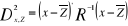 (1) (1)
With x the vector of length p, representing
the values of the three environmental triplets to be tested
(j=2,530,206), Rp,p the correlation matrix of
reference matrix Zm,p and  the average environmental condition inferred from
Zm,p. There were as many calculations of the
Mahalanobis generalised distance as environmental triplets to be tested
(j=2,530,206). These triplets were chosen in such a way to cover the entire
ecological niche of the species or its entire spatial distribution (see Figs.
III.S1, III.1 and III.4). Many ecological niche models are based on the
Mahalanobis generalised distance (Farber & Kadmon 2003; Calenge et
al. 2008; Nogués-Bravo et al. 2008). However, the novelty
lies in the fact that the model offers a new way to calculate the probability
of the Mahalanobis generalised distance using a non parametric procedure. the average environmental condition inferred from
Zm,p. There were as many calculations of the
Mahalanobis generalised distance as environmental triplets to be tested
(j=2,530,206). These triplets were chosen in such a way to cover the entire
ecological niche of the species or its entire spatial distribution (see Figs.
III.S1, III.1 and III.4). Many ecological niche models are based on the
Mahalanobis generalised distance (Farber & Kadmon 2003; Calenge et
al. 2008; Nogués-Bravo et al. 2008). However, the novelty
lies in the fact that the model offers a new way to calculate the probability
of the Mahalanobis generalised distance using a non parametric procedure.
Figure III.2 : Ecological niches
estimated after hoogenization (i.e. correction) of the original training set
according to three environmental parameters: sea surface temperature (SST, left
panels), bathymetry (middle panels) and sea surface salinity (SSS, right
panels). (a) Atlantic horse mackerel, (b)
European anchovy, (c) European sprat, (d)
pollack, (e) common sole, (f) haddock,
(g) saithe and (h) turbot. The number of
observations was log10 transformed for bathymetry.
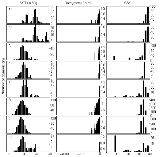
To calculate the probability of significance of the distance,
each observation of the reference matrix Zm,p was
permuted to become the observation to be tested and the original tested
observation was included to the reference matrix. The Mahalanobis generalised
distance was then recalculated for each permutation. The number of total
permutations was equal to m. A probability w can then be assessed by looking at
the number of times the simulated distance was found to be superior or equal to
the observed distance between the observation and the reference matrix
Zm,p. The probability was calculated as follows:
 (2) (2)
Where the probability w was the number of times the simulated
Mahalanobis generalised distance ds was found to be superior or
equal to the observed mean distance do. When w tends towards 1, the
observation has environmental conditions that represent the centre of the
species niche. When w tends towards 0, the observation has environmental
conditions outside the species niche. It is important to have a large reference
matrix Zm,p so that the resolution of the
probability is as high as possible. Such a procedure was performed for each of
the j=2,530,206 observations and all 8 species.
Step 6: Evaluation of the model as a
function of different simulated training sets
The model can be used to assess the ecological niche of a
species. Before calculating the spatial pattern of changes in the probability
of fish occurrence, we evaluated how the model reacted to different kind of
simulated training sets: (1) homogeneous (considered here as the set of
reference); (2) nearly-homogeneous; (3) symmetrical bimodal; (4) asymmetrical
bimodal (see Fig. III.3), therefore simulating some observed ecological niches
(see Fig. III.2). The mean difference D between the set of reference R and the
simulated training set S was assessed as follows:
 (3) (3)
With 0=D=1, n the number of probabilities to be compared,
Ri the ith probability of the set of reference and
Si the ith probability of the simulated training set.
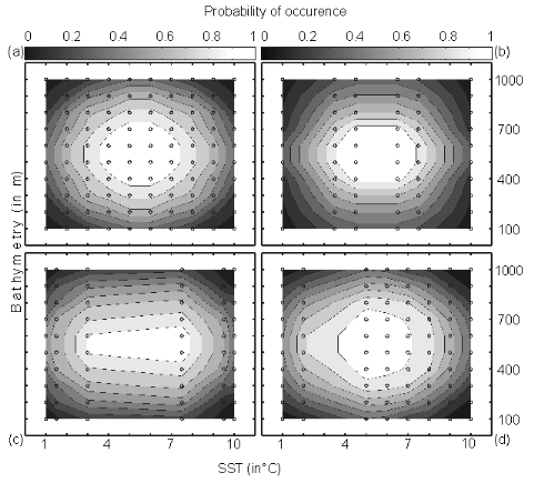
Step 7: Application of the model
for different sets of environmental conditions
The model was then applied on the corrected training set (see
Step 3) with as environmental variables, the bathymetry and annual SSS (assumed
to be constant over the period) and both observed and projected annual SST.
Spatial distributions (see Figs. III.4 and III.S12 to III.S19) were provided
for the period 1960-1969, the period 2000-2005 (observed SST data) and the
decades 2050s and 2090s (projected SST data, see Fig. III.S11 to III.S19).
Step 8: Statistical analyses of
the results
Comparison of the models NPPEN and AquaMap
Figure II. 3
For each species, a correlation analysis was applied to
compare the maps of probability of fish occurrence inferred from the AquaMap
approach of Kaschner and colleagues (a modified version of the Relative
Environmental Suitability model of Kaschner et al. 2006) and the model NPPEN.
This comparison was performed on maps based on annual SST averaged for the
period 1960-2005. To evaluate the impact of spatial autocorrelation when the
correlation was calculated between maps, the minimum degree of freedom needed
to have a significant correlation (p=0.05) was also assessed (Beaugrand &
Helaouët 2008).
Figure III.3 : Probability of occurrence
calculated using NPPEN from two variables (bathymetry and annual sea surface
temperature (SST). (a) Reference training set with occurrence
points (as circle) and associated probability (shaded grey),
(b) simulated training set 1 (central gap in occurrence
points), (c) simulated training set 2 (large central gap and
slight asymmetry in occurrence points) and (d) simulated
training set 3 (pronounced asymmetry in occurrence points).
Quantification of long-term changes in potential species
distribution
To quantify the potential long-term changes in species
distribution, probabilities of occurrence for the periods 1960-1969, 2000-2005
and 2090-2099 (scenarios A2 and B2) were converted into binary data. The
presence was considered as certain when the probability of occurrence for a
species was =0.2 (threshold selected by trial and error; different thresholds
were selected and gave similar conclusions) and a value of 1 was attributed.
Below this threshold, a 0 was ascribed. The differences between the 2000-2005
and 1960-1969 and the period 2090-2099 (for scenarios A2 and B2) and 1960-1969
were then calculated. A positive difference (quantified in km²) was
interpreted as a gain of potential habitat and inversely. The surface A was
calculated by assimilating the geographical cell to an isosceles trapeze:
 (4) (4)
With g being the longitudinal distance (in km) between the two
minimum latitudes of the trapeze, s the longitudinal distance (in km) between
the two maximum latitudes of the trapeze, l the distance between the maximum
and minimum latitude on the western part of the trapeze and r the distance
between the maximum and minimum latitude on the eastern part of the trapeze.
The four distances were assessed as follows (Beaugrand & Ibañez,
2002):
d(i,j)=6377.221 x hi,j (5)
With di,j being the geographical distance between
point i and j, the constant the Earth radius and hi,j computed as
follows (Beaugrand & Ibañez 2002):
 (6) (6)
With öi the latitude (in radians) at point i,
öj the latitude (in radians) at point j and g the difference in
longitude between i and j.
2.4. Results
? Estimation of the realised niche from uncorrected
and corrected reference matrices
Data occurrences from the uncorrected training sets were first
used to determine the realised niche of each fish (Fig. III.S10). The contours
of these niches depended on species. Some species exhibited a unimodal
distribution close to a normal distribution. For example, the examination of
the thermal tolerance of haddock (Fig. III.S10(f)) showed a preferendum ranging
between 5°C and 15°C and an optimum around 9.75°C. Pollack was
more stenotherm, found between 9°C and 15°C with a thermal optimum at
about 12.75°C (Fig. III.S10(d)). However, for other species and
parameters, the distribution could be multimodal (e.g. Atlantic horse mackerel
and European anchovy; see Fig. III.S10(a), (b)). For all species, the
bathymetric distribution did not follow a normal distribution. The frequencies
of occurrence were maximal for the first 200 meters (i.e. continental shelf).
The contours of the niche for annual SSS were not as well defined as for the
other parameters because the amplitude of variation in the region was not
generally important. All species showed mainly a maximum of occurrence between
30 and 40. Pollack was less euryhaline than species such as common sole and
turbot (Fig. III.S10(e), (h)). The different salinity profiles exhibited by the
species highlighted the importance of the parameter as a predicting variable in
NPPEN.
Multiple modes are less conform to our common idea of the
ecological niche. They can be related to the absence of a specific habitat or
to the presence of oversampled or undersampled regions. They could also be due
to seasonal migration such as the one performed by sardine. Indeed most often,
data used in ENMs do not originate from rigorous sampling protocol (Legendre
& Legendre 1983). To consider this bias, the training set was corrected,
which resulted in an improvement of most environmental preferendums (Fig.
III.2). However, the procedure of correction did not modify substantially the
environmental profiles of species, indicating that the profiles were here not
too much influenced by the heterogeneity of the spatial information. Most
optimums were refound (Fig. III.2). In the case of poorer occurrence dataset
(e.g. turbot; Figs. III.S10(h) and 2(h)), the correction allowed contours of
the salinity preferendum to be completed. This homogenisation procedure enabled
some response curves to be better balanced. Such a correction was essential as
most ENMs, as ours, are highly sensitive to the determination of the niche
? Sensitivity of the model to bimodality and sampling
density
Previous results showed that some species exhibited multimodal
responses (Figs. III.S10 and 2). To evaluate the influence of such
patterns on our model, we simulated training sets characterised by different
types of bimodality and sampling density (Fig. III.3). This comparisonwas made
by simulating the values of two environmental parameters: SST and bathymetry.
When the density of sampling was regular and in case of unimodality, the
highest probabilities were observed at the centre of the sampling points and
declined progressively towards the edge of the distribution (Fig. III.3(a)).
This training set was considered here as a reference to evaluate simulated
incomplete, heterogeneous and bimodal training sets. The model was robust to
incomplete or heterogeneous training sets (Fig. III.3). The mean difference
ranged from 0.0940 (Fig. III.3(b)), 0.0732 (Fig. III.3(c)) to 0.0622
(Fig. III.3(d)). These results suggest that the model was quite robust to
altered training set that could be related to incomplete sampling coverage or
an unrepresented biotope.
Figure III.4 : Estimated probability of
occurrence using the model NPPEN for the decade 1960-1969, the time period
2000-2005 in the North Atlantic Ocean. (a) Atlantic horse
mackerel, (b) European anchovy, (c) European
sprat, (d) pollack, (e) common sole,
(f) haddock, (g) saithe and
(h) turbot. The western boundary of the model was fixed to
40°W. This was arbitrary selected for species (but haddock and saithe),
which are only found on the eastern side of the Atlantic Ocean.
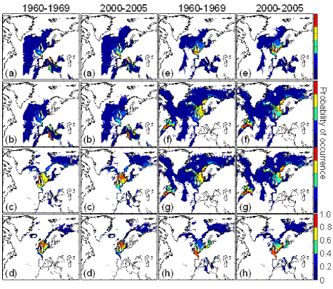
? Modelled spatial distribution of fish species
(contemporaneous spatial patterns)
The examination of the modelled spatial distribution for the 8
species considered in this study indicated the presence of three groups (Fig.
III.4, period 1960-1969): (1) species with a spatial distribution mainly
centred in the Celtic Sea and/or the North Sea (called temperate species;
European sprat, pollack and turbot); (2) species with a spatial distribution
from southerly regions to the North Sea (called warm-temperate species;
Atlantic horse mackerel, European anchovy and common sole); (3) species with a
spatial distribution ranging from the North Sea to the Barents Sea (called
subarctic species; haddock and saithe). These results showed that the North Sea
and more generally regions close to the British Isles represented a
biogeographical crossroad between the Atlantic Arctic and the Atlantic
Westerlies Wind (temperate) biomes (Longhurst 1998). The probability of fish
occurrence calculated from NPPEN exhibited substantial differences with the
maps produced by the FAO (Fig. III.S1).
? Comparison of the spatial distribution inferred from
NPPEN and AquaMap
We compared the spatial distribution of fish occurrence
modelled by NPPEN for the 1960s and the period 2000-2005 with outputs from
AquaMap (Kaschner et al. 2006) by correlation analysis (Table III.1).
The strength of the correlations, similar for the two periods (190-1969, mean
correlation: 0.5075; 2000-2005, mean correlation: 0.53), depended on species.
Although all coefficients of correlation were significant, the amount of
variance explained ranged from 1.44% for European anchovy to 56.25% for haddock
(Table III.1). The minimum degree of freedom needed to have a significant
correlation was calculated to evaluate in which measure the spatial
autocorrelation could have influenced the results. For example, the high
correlation found with haddock remained significant (p= 0.05) with only 5
degree of freedom (Table III.1). The reduction of the degree of freedom ranged
from 5 to 255 (European anchovy). In general, the correlation between the two
models tended to increase with the number of occurrence data in the reference
matrix (correlation calculated between the decimal logarithm of the number of
data after simplification of the training set in Supplementary Table III.1 and
correlation coefficients in Table III.1; 1960-1969: rp=0.53, p=0.17;
2000-2005: rp=0.45, p=0.27).
Figure III.5 : Maps showing areas where
a substantial increase (in red) or decrease (in blue) in the probability of
occurrence (changes>0.2, see `Materials and methods') is expected between
the 2090s and the 1960s. Green areas denote no substantial change or changes
<0.2. (a) Atlantic horse mackerel, (b)
European anchovy, (c) European sprat, (d)
pollack, (e) common sole, (f) haddock,
(g) saithe and (h) turbot. The western
boundary of the model was fixed to 40°W. This was arbitrary selected for
species (but haddock and saithe), which are only found on the eastern side of
the Atlantic Ocean.
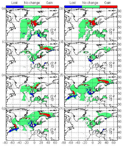
Table III.1 : Correlations between the
spatial patterns in the probability of fish occurrence between the model NPPEN
and AquaMap (Kaschner et al. 2006) for the period 1960-1969 and
2000-2005. n: degree of freedom; rp: Pearson linear coefficient of
correlation; p: probability; n.f.: minimum degree of freedom needed to have a
significant correlation at p=0.05.
|
|
NPPEN 1960/1969 - AquaMap
|
NPPEN 2000/2005 - AquaMap
|
|
Row
|
FAO species names
|
N
|
rp
|
p
|
n.f.
|
n
|
rp
|
p
|
n.f.
|
|
(a)
|
Atlantic Horse mackerel
|
63,021
|
0.49
|
<0.01
|
14
|
62,904
|
0.54
|
<0.01
|
11
|
|

(b)
|
European Anchovy
|
58,831
|
0.12
|
<0.01
|
255
|
58,722
|
0.14
|
<0.01
|
184
|
|
(c)
|
European Sprat
|
30,582
|
0.47
|
<0.01
|
15
|
30,503
|
0.47
|
<0.01
|
16
|
|
(d)
|
Pollack
|
19,865
|
0.71
|
<0.01
|
5
|
19,854
|
0.68
|
<0.01
|
6
|
|
(e)
|
Common Sole
|
41,029
|
0.52
|
<0.01
|
12
|
40,883
|
0.60
|
<0.01
|
8
|
|
(f)
|
Haddock
|
86,820
|
0.75
|
<0.01
|
5
|
86,286
|
0.72
|
<0.01
|
5
|
|
(g)
|
Saithe
|
76,009
|
0.61
|
<0.01
|
8
|
75,689
|
0.61
|
<0.01
|
8
|
|
(h)
|
Turbot
|
26,923
|
0.39
|
<0.01
|
23
|
26,796
|
0.48
|
<0.01
|

15
|
|
Row
|
FAO species names
|
Thermal preference
|
Period 2000/2005 ? 1960/1969
|
Period 2090/2090 ? 1960/1969
Scenario A2
|
Period 2090/2099 ? 1960/1969
Scenario B2
|
|
|
|
Gain
|
Lost
|
Balance
|
Gain
|
Lost
|
Balance
|
Gain
|
Lost
|
Balance
|
|
(a)
|
Atlantic horse mackerel
|
Warm temperate
|
173,865
|
56,125
|
117,740
|
956,524
|
969,816
|
?13,291
|
918,117
|
737,099
|
181,017
|
|
(b)
|
European anchovy
|
Warm temperate
|
375,539
|
29,205
|
346,334
|
1,020,267
|
39,302
|
980,965
|
984,187
|
17,768
|
966,419
|
|
(c)
|
European sprat
|
Temperate
|
285,696
|
83,857
|
201,839
|
601,395
|
419,186
|
182,209
|
598,114
|
328,168
|
269,946
|
|
(d)
|
Pollack
|
Temperate
|
36,505
|
47,779
|
?11,274
|
101,459
|
352,090
|
?250,631
|
56,010
|
315,461
|
?259,451
|
|
(e)
|
Common sole
|
Warm temperate
|
105,455
|
23,381
|
82,074
|
430,869
|
430,972
|
?102
|
435,829
|
321,902
|
113,926
|
|
(f)
|
Haddock
|
Sub-Arctic
|
341,083
|
266,414
|
74,668
|
899,733
|
1,311,603
|
?411,870
|
794,319
|
1,189,764
|
?395,445
|
|
(g)
|
Saithe
|
Sub-Arctic
|
281,311
|
278,110
|
3,200
|
908,634
|
1,503,825
|
?595,190
|
796,864
|

1,295,440
|
?498,576
|
|
(h)
|
Turbot
|
Temperate
|
59,873
|
101,639
|
?41,766
|
154,142
|
334,280
|
?180,138
|
147,409
|
216,425
|
?69,016
|

Table III.2 : Thermal preference and the
expected area (in km²) gained or lost by the species between the period
2000-2005 and 1960-1969 and 2090-2099 and 1960-1969 for both scenarios A2 and
B2. The balance was calculated (in km²) as the difference between gained
and lost area (see Materials and Methods).
? Observed changes in species distribution
All species but haddock exhibited a northward movement or an
increase in the probability of occurrence at the northern edge of their spatial
distribution between the 1960s and the period 2000-2005 (Fig. III.4). The
probability of occurrence of European sprat increased substantially in the
North Sea in 2000-2005. The reduction in the probability at the southern edge
of all species was not evident with the exception of European sprat, saithe and
haddock (e.g. the southern part of the North Sea). Between the 1960s and the
period 2000-2005, the potential habitat of warm-temperate species increased
(Table III.2). Among them, the potential habitat of European anchovy increased
substantially (balance of change: 346,334 km²). Both subarctic and
temperate species exhibit a weak or a moderate increase between the 1960s and
the period 2000-2005 or a moderate decrease for pollack and turbot (Table
III.2).
? Changes in species distribution
Modelled spatial distributions based on projected IPCC changes
in SST (scenario B2) suggest that northward movements in fish may accelerate in
the future with the exception of pollack in the North Sea (Fig. III.S10). These
movements will be generally associated with a reduction located at the southern
edge of the species spatial distribution (Fig. III.S10). The projections
suggest that the potential habitat of European anchovy will increase (Fig.
III.5, Table III.2). Results are less obvious for common sole or Atlantic horse
mackerel and suggested either a weak decrease (Scenario A2, Table III.2) or a
moderate increase (Scenario B2, Table III.2). Atlantic horse mackerel and
European anchovy are expected to move northwards along the European shelf-edge
and in the North Sea (Figs. III.S10 and III.5, Table III.2). The potential
habitat of temperate species is expected to decrease substantially
(Fig. III.5, Table III.2) with the exception of European sprat that is
expected to migrate to the Barents Sea. However, this species might eventually
disappear from the central part of the North Sea at the end of the century
(Fig. III.S10). The model suggests that the potential habitat of subarctic
species may diminish considerably (Fig. III.5, Table III.2). The reduction of
the potential habitat in the North Sea may not be overcome by the increase in
potential habitat over the Barents Sea. Projections based on scenario A2 and B2
for subarctic species gave very similar conclusions (Table III.2).
2.5. Discussion
Our use of an ENM to determine the potential geographical
range of a species excludes fundamental biotic interactions or processes
related to resource availability. Indeed, process models enable physiological
constraints, population dynamics, life history traits and trophic interactions
to be considered (Speirs et al. 2006). However, such detailed
knowledge is rarely available (Carpenter et al. 1993). The large scale
at which our study was conducted overcomes partly this drawback, trophic
interactions being for example more important at a local scale (Pearson &
Dawson 2003). We chose to base our projections on a limited number of
parameters for the following reasons: (1) too many parameters increase the risk
of multicollinearity, which could prevent the calculation of the Mahalanobis
generalised distance; (2) the number of samples needed in the reference matrix
increases when the number of parameters augments; (3) A high number of
parameters would also increase the uncertainties of the model. We did not
consider habitat characteristics (e.g. sediment type), essential for common
sole and turbot. Indeed, it was assumed that climate exerts its major influence
on fish through the effects of temperature on larval development since the
larval stage is a critical life cycle phase affecting recruitment (Cushing
1996). Although adult species selected in this study are pelagic, demersal or
benthic, all have a pelagic stage. Therefore, our result should be more
interpreted as reflecting the potential habitat of a species, without the
influence of the type of sediments (Amara et al. 2004) or processes
such as trophic interactions or dispersal (Pulliam 2000).
It should be reminded that the optimal part of the realised
niche (sensu Hutchinson, 1957) was inferred from the frequency of
occurrence of each species in a particular stratum. A clear assumption in our
technique, as in other modelling techniques based on presence-only data, is
that the maximum frequency of occurrence occurs at the optimal part of the
realised niche. It is thereby expected that a too scarce sampling may deform
the realised niche and bias our projection. This is the reason why we based on
projection on a large number of datapoints (Supplementary Table III.1) and
represented the realised niche of all species to examine if the whole niche was
covered (Figs. III.S10 and III.2). Furthermore, the technique is not sensitive
to spatial scarcity of the data but rather to an incomplete assessment of the
preferendum of a species. We have to know sufficiently well the niche to
project the spatial distribution of the species.
The quality of the data is a fundamental parameter affecting
the dependability of results of ENMs (Stockwell & Peterson 2002). Contrary
to the terrestrial realm, the marine biosphere is more difficult to sample and
the joint information on presence and absence is rare. Therefore, ENMs
requiring presence/absence data such as Generalised Additive Models (GAM;
Hastie & Tibshirani 1990) or Generalised Linear Models (GLM; McCullagh
& Nelder 1983) although representing powerful tools and often producing
better predictions than presence-only evaluators (Brotons et al. 2004)
are inappropriate. Ecological Niche Factor analysis (ENFA; Hirzel 2001),
AquaMap (Kaschner et al. 2006), the maximum entropy modelling (MAXENT;
Phillips et al. 2006), BIOCLIM, HABITAT and DOMAIN are some of the
techniques applied when only-presence data are available (Carpenter et
al. 1993).
The comparison of the model NPPEN with the one of Kaschner
et al. (2006) indicated that although for some species the correlation
was high (see Table III.1), substantial differences might occur for some
species (e.g. European anchovy and pollack). Such differences may be related to
the inherent property of the model (e.g. the difference of objectivity between
the two techniques), the number and the choice of the environmental parameters
or the number of samples (see the correlations between the two models and the
number of samples) to have a representative training set. AquaMap is more
dependent on expert knowledge and the contour of the trapezoidal model is often
fixed from biological expertise. One of the main advantages of the technique
NPPEN is that it is nonparametric, contrary to ENFA (Hirzel et al.
2006), does not require the selection of underlying functions as in MAXENT
(Phillips et al. 2006) and parametrisation or the attribution of
thresholds as in AquaMap (Kaschner et al. 2006), ENFA and MAXENT.
However, the analysis is dependent, as most of the current available
techniques, upon a correct assessment of the ecological niche and is highly
dependent of the quality of the training set (especially the contour of the
niche, see Fig. III.3). A too high number of outliers might have a strong
influence on probability (Beaugrand et al. submitted). This drawback
can be overcome by the use of the procedure of homogenisation with an
increasing threshold (threshold of presence data in an environmental
stratum=2). However, caution is needed as the homogenisation can lead to an
underassessment of the width of the niche.
The probability from our model is unlikely to have been
strongly influenced by spatial autocorrelation (SAC; Segurado et al.
2006; Dormann 2007), likely to occur in environmental parameters such as annual
SST. Spatial autocorrelation increases the Type I error rate which leads to the
incorrect rejection of the null hypothesis of no effect. SAC is likely to
affect more strongly regression techniques such as GLMs and GAMs and some
adjustments are being developed to overcome this problem (Dormann et
al. 2007). However, the impact of SAC remains uncertain for some authors
(Diniz-Filho et al. 2003). The determination of SAC was not undertaken
in this study. However, the step of homogenisation (or adjustment of the
training set) we applied in this study have probably strongly limit the
influence of SAC on probability. Such procedure, which reduces
pseudo-replication, is congruent with recommendations of some authors
(Brito et al. 1999; Stockwell & Peters 1999; Guisan &
Zimmermann 2000; Segurado et al. 2006).
The influence of climate change on marine ecosystems and more
particularly on species distribution has become prominent (Intergovernmental
Panel on Climate Change 2007a). In this context, there is an urgent need to
better assess the spatial distribution of species for conservation and
management issues (Parmesan 2006). The new model NPPEN was used to estimate the
past, current and potential future changes in species distribution of some
marine fish commercially exploited in the North Atlantic sector. The new maps
of spatial distribution provide quantitative information on spatial
distribution often presented as categorical or binary maps (FAO;
http://www.fao.org/fi/figis/maps/compilat.htm
and (Louisy 2002). The new model also gives alternative views on quantitative
spatial distribution recently provided by Cheung et al. (2008a, 2008b,
2009) using a new dynamic bioclimate envelope model or by the method AquaMap
(Kaschner et al. 2006) used in FishBase (Froese & Pauly 2009).
One important assumption when modelled SST data is that there
is no discrepancy between observed SST (ICOADS) and modelled SST (ECHAM 4).
Beaugrand et al. (2008) compared observed ICOADS and ECHAM 4 modelled
data for the period 1990-2005. Modelled and observed data on annual SST were
highly positively correlated in the area covered by this study (r=0.95,
p<0.0001, n=1809), showing that the model ECHAM 4 captures relatively well
the complexity of the hydro-climatic environment of the North Atlantic at a
decadal scale. All modelled spatial distributions explain current observed
large-scale changes in fish distribution (e.g. Perry et al. 2005; Rose
2005; Kirby et al. 2006; Hiddink & Ter Hofstede 2008; Cheung
et al. 2008b, 2009). Overall, results show a migration of marine resources
polewards at rate varying among species, agreeing with other studies based on
observational data (Quero et al. 1998; Brander et al. 2003;
Perry et al. 2005; Kirby et al. 2006). Northward movements
are clearly detected for most species with potential habitat gained at the
northern edge of the spatial distribution and potential habitat lost at their
southern edge. Brander (2003) also noted this northward movement for commercial
gadoid and flatfish. They found however some examples of southward shifts that
he explained by local hydrodynamical characteristics (e.g. sardine in upwelling
regions off Portugal). Furthermore, Perry et al. (2005) investigating
long-term spatial changes in 36 species found that about two-thirds of both
commercial and non-commercial species shifts their spatial distribution
northwards in the North Sea as a response to sea temperature warming. The
authors observed that some species moved in deeper regions, suggesting that
some species may adapt to temperature warming by moving vertically. This effect
was not accounted for in our statistical model.
Perhaps more interestingly, our results indicate that some
species may not be able to track their environmental envelop and could loss a
significant amount of their habitats (Fig. III.5 and Table III.2: pollack)
as they might be restricted by other specific local or regional constraints
related to the bathymetry (e.g. flatfish). Of some interests, the model
explains the pronounced increase in the abundance of European sprat in the
Baltic Sea and the North Sea since the 1990s, which has had some influence on
some seabird species (Österblom et al. 2008; Wanless et
al. 2005). For example, the increase in the stock of European sprat in the
Baltic Sea has led to a decrease in energetic content (Österblom et
al. 2006). These authors showed how this loss in quality food caused loss
in fledging mass of common guillemot chicks. Our model could be applied on
sandeels to examine whether a decrease in the probability of occurrence of this
species paralleled the increase in European sprat.
Our results show that the general latitudinal movement in fish
distribution detected for past decades may accelerate (Fig. III.S11, Table
III.2). More sustained warming could trigger more rapid northward shifts.
Associated with fishing, climate-induced shifts could have a strong impact on
socio-economical systems by precipitating the collapse of some stocks,
especially at the southern edge of current species distribution (Beaugrand
et al. 2008). Other regions (e.g. the Barents Sea) will see a pronounced
increase in their potential habitat. However, relaxed fishing pressure due to
an improved ecosystem carrying capacity might mitigate the potential for growth
in fish stocks (e.g. gadoids in the Barents Sea). The uncertainties related to
these projections are obviously high and perhaps more importantly cannot at
present be assessed with confidence. These uncertainties are related to the
climatic scenario itself (scenario A2 and B2), the uncertainties of the
physical model (here the ECHAM 4 model) and limitations of our own model. Many
other uncertainties remain and the complexity of the system makes it difficult
to consider these maps as exact predictions but rather as projections of
potential distribution in the absence of biotic interactions, dispersal and
processes related to population dynamics which cannot be realistically
considered with our current level of knowledge. Nevertheless, ENMs might
provide a new management tool against which changes in the resource might be
better anticipated and improve sustainable exploitation strategy in the context
of rapid global climate change associated to pronounced anthropogenic impact on
the marine biosphere.
Acknowledgments
We are grateful to all past and present members and supporters
of the FishBase website (
http://www.FishBase.org), whose
continuous efforts have allowed the establishment of the fish data set. We
thank Dr Keith Brander for helpful comments on an early version of the
manuscript. The research was supported by the French Agency of Research and
Technology (ANRT, grant CIFRE 862/2007).
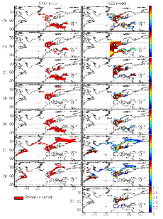
Supporting
Information
Figure III.S1 : Spatial distribution of
species selected in this study inferred from the FAO geographical distribution
model (left) and the AquaMap approach (right, Kaschner et al., 2006).
(a) Atlantic horse mackerel, (b) European
anchovy, (c) European sprat, (d) pollack,
(e) common sole, (f) haddock,
(g) saithe and (h) turbot. The FAO model
illustrates the predicted distribution area of marine fish from a GIS approach.
Red areas represent regions where the presence of the species is considered as
certain. No FAO map for turbot was available. The RES model represents the
probability of species presence (between 0 and 1).
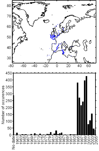
Figure III.S2 : Spatial and temporal
distribution of occurrences datapoints for Atlantic horse mackerel used to
assess the spatial distribution of species.

Figure III.S3 : Spatial and temporal
distribution of occurrence datapoints for European anchovy used to assess the
spatial distribution of species.
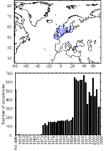
Figure III.S4 : Spatial and temporal
distribution of occurrence datapoints for European sprat used to assess the
spatial distribution of species.
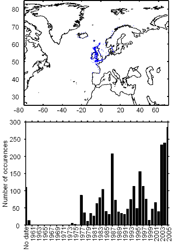
Figure III.S5 : Spatial and temporal
distribution of occurrence datapoints for pollack used to assess the spatial
distribution of species.
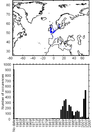
Figure III.S6 : Spatial and temporal
distribution of occurrence datapoints for common sole used to assess the
spatial distribution of species.
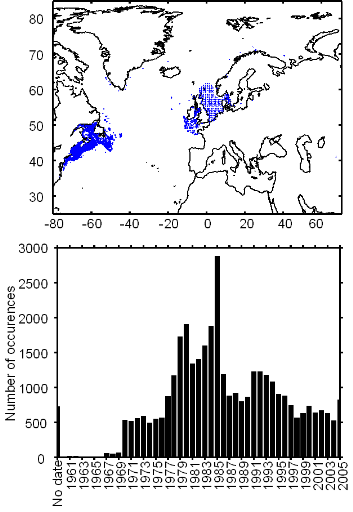
Figure III.S7 : Spatial and temporal
distribution of occurrence datapoints for haddock used to assess the spatial
distribution of species.
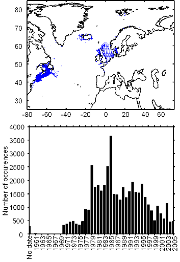
Figure III.S8 : Spatial and temporal
distribution of occurrence datapoints for saithe used to assess the spatial
distribution of species.
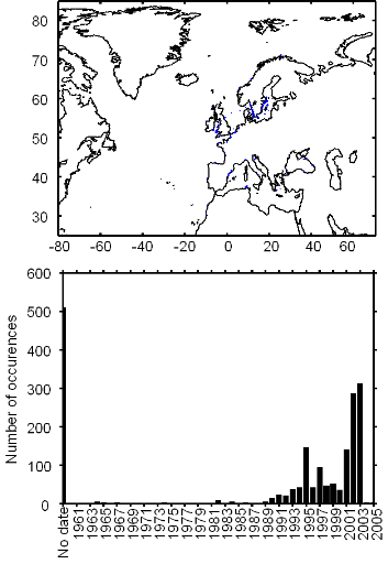
Figure III.S9 : Spatial and temporal
distribution of occurrence datapoints for turbot used to assess the spatial
distribution of species.
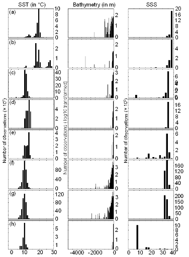
Figure III.S10 : Ecological niches
(sensu Hutchinson 1957) estimated from the occurrence data of the
original (uncorrected) training set and as a function of three environmental
parameters: annual sea surface temperature (SST, left panels), bathymetry
(middle panels) and annual sea surface salinity (SSS, right panels).
(a) Atlantic horse mackerel, (b) European
anchovy, (c) European sprat, (d) pollack,
(e) common sole, (f) haddock,
(g) saithe and (h) turbot.


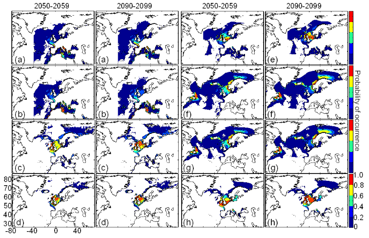
Figure III.S11 : Estimated probability of
occurrence using the model NPPEN for the decade 2050-2059 and 2090-2099
(scenario B2) in the North Atlantic Ocean. (a) Atlantic horse
mackerel, (b) European anchovy, (c) European
sprat, (d) pollack, (e) common sole,
(f) haddock, (g) saithe and
(h) turbot. The western boundary of the model was fixed to
401W. This was arbitrary selected for species (but haddock and saithe) which
are only found on the eastern side of the Atlantic Ocean.
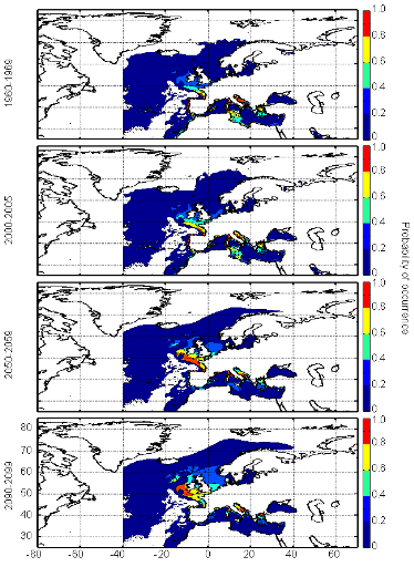
Figure III.S12 : Estimated probability of
occurrence of Atlantic horse mackerel using the model NPPEN for the decade
1960-1969, the time period 2000-2005 and for the decades 2050-2059 and
2090-2099 (scenario B2) in the North Atlantic Ocean.
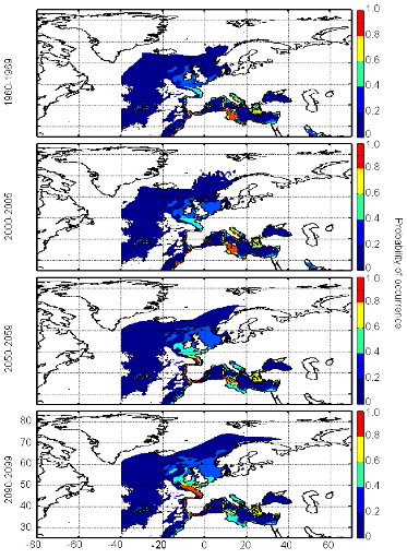
Figure III.S13 : Estimated probability of
occurrence of European anchovy using the model NPPEN for the decade 1960-1969,
the time period 2000-2005 and for the decades 2050-2059 and 2090-2099 (scenario
B2) in the North Atlantic Ocean.
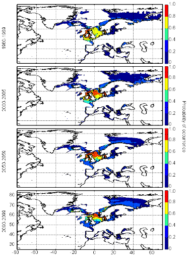
Figure III.S14 : Estimated probability of
occurrence of European sprat using the model NPPEN for the decade 1960-1969,
the time period 2000-2005 and for the decades 2050-2059 and 2090-2099 (scenario
B2) in the North Atlantic Ocean.
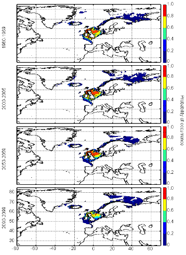
Figure III.S15 : Estimated probability of
occurrence of pollack using the model NPPEN for the decade 1960-1969, the time
period 2000-2005 and for the decades 2050-2059 and 2090-2099 (scenario B2) in
the North Atlantic Ocean.
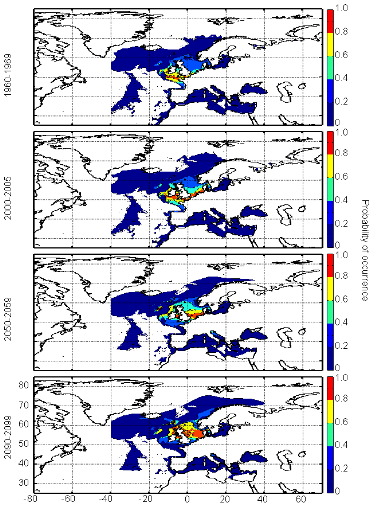
Figure III.S16 : Estimated probability of
occurrence of common sole using the model NPPEN for the decade 1960-1969, the
time period 2000-2005 and for the decades 2050-2059 and 2090-2099 (scenario B2)
in the North Atlantic Ocean.
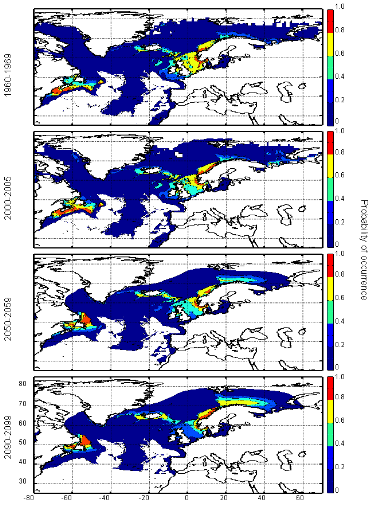
Figure III.S17 : Estimated probability of
occurrence of haddock using the model NPPEN for the decade 1960-1969, the time
period 2000-2005 and for the decades 2050-2059 and 2090-2099 (scenario B2) in
the North Atlantic Ocean.
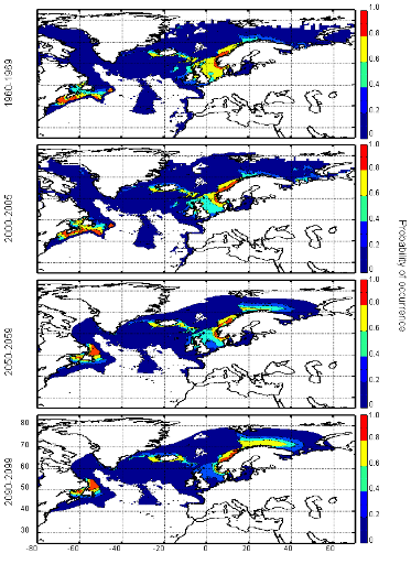
Figure III.S18 : Estimated probability of
occurrence of saithe using the model NPPEN for the decade 1960-1969, the time
period 2000-2005 and for the decades 2050-2059 and 2090-2099 (scenario B2) in
the North Atlantic Ocean.
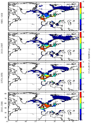
Figure III.S19 : Estimated probability of
occurrence of turbot using the model NPPEN for the decade 1960-1969, the time
period 2000-2005 and for the decades 2050-2059 and 2090-2099 (scenario B2) in
the North Atlantic Ocean.
TableIII.S1 : List of marine fish species
used in this study with their official FAO and scientific names. The
bathymetric preference for each species was obtained from Louisy (2002) and
FishBase (Froese & Pauly, 2009;
http://www.FishBase.org). The
number of occurrence points before (left) and after (right) the attribution of
environmental variables is indicated, showing the reduction in the data because
of missing environmental data.
|

Row
|
FAO species names
|
Scientific names
|
Bathymetric preferences
|
Number of data
Before/After
|
|
|
|
|
|
|
(b)
|
European anchovy
|
Engraulis encrasicolus (Linnæus, 1758)
|
Pelagic
|
1,631/ 813
|
|
(c)
|
European sprat
|
Sprattus sprattus sprattus (Linnæus, 1758)
|
Pelagic
|
11,072/ 9,866
|
|
(d)
|
Pollack
|
Pollachius pollachius (Linnæus, 1758)
|
Benthopelagic
|
2,596/ 1,910
|
|
(e)
|
Common sole
|
Solea solea (Linnæus, 1758)
|
Demersal
|
4,322/ 1,137
|
|
(f)
|
Haddock
|
Melanogrammus aeglefinus (Linnæus, 1758)
|
Demersal
|
36,733/ 35,584
|
|
(g)
|
Saithe
|
Pollachius virens (Linnæus, 1758)
|
Demersal
|

45,212/ 40,787
|
|
(h)
|
Turbot
|
Psetta maxima (Linnæus, 1758)
|
Demersal
|
1,864/ 1,308
|
Supplementary Table III.1 Lenoir et al.
Annexe :
Atlas climatique des ressources marines de l'Atlantique
Nord
Conjointement à cette étude, il a
été réalisé un atlas des distributions spatiales et
des changements attendus de ces distributions pour 51 espèces marines en
Atlantique Nord, en utilisant le nouveau modèle NPPEN. Cet atlas est le
fruit d'une collaboration avec SEAFISH industrie. Une présentation de
l'atlas et un exemple des cartes de distribution y figurant ont
été inclus en annexe, à la fin de ce chapitre.
A climatic atlas of North Atlantic marine resources
with a special emphasis on the English Channel and the North Sea
Sylvain Lenoir, Grégory Beaugrand
1 Centre National de la Recherche Scientifique,
Laboratoire d'Océanologie et de Géosciences'
UMR LOG CNRS 8187, Station Marine, Université des
Sciences et Technologies de Lille - Lille 1, BP 80, 62930 Wimereux, France
E-mail:
sylvain.lenoir@ed.univ-lille1.fr,
Gregory.Beaugrand@univ-lille1.fr
Report Contract for SEAFISH
31 Décembre 2008
How the two documents should be cited:
Beaugrand G, Lenoir S (2008) A climatic atlas of North Atlantic
marine resources with a special emphasis on the English Channel and the North
Sea. Introduction and description of the procedures. Technical Report. Centre
National de la Recherche Scientifique. Station Marine de Wimereux.
Université des Sciences et Technologies de Lille 1. 17 pages.
Lenoir S, Beaugrand G (2008) A climatic atlas of North Atlantic
marine resources with a special emphasis on the English Channel and the North
Sea. Technical Report. Centre National de la Recherche Scientifique. Station
Marine de Wimereux. Université des Sciences et Technologies de Lille 1.
515 pages.
A climatic atlas of North Atlantic marine resources
with a special emphasis on the English Channel and the North Sea
Introduction and description of the
procedures
Grégory Beaugrand, Sylvain Lenoir
1 Centre National de la Recherche Scientifique,
Laboratoire d'Océanologie et de Géosciences'
UMR LOG CNRS 8187, Station Marine, Université des
Sciences et Technologies de Lille - Lille 1, BP 80, 62930 Wimereux, France
E-mail:
Gregory.Beaugrand@univ-lille1.fr,
sylvain.lenoir@ed.univ-lille1.fr
Report Contract for SEAFISH
31 Décembre 2008
How the two documents should be cited:
Beaugrand G, Lenoir S (2008) A climatic atlas of North Atlantic
marine resources with a special emphasis on the English Channel and the North
Sea. Introduction and description of the procedures. Technical Report. Centre
National de la Recherche Scientifique. Station Marine de Wimereux.
Université des Sciences et Technologies de Lille 1. 17 pages.
Lenoir S, Beaugrand G (2008) A climatic atlas of North Atlantic
marine resources with a special emphasis on the English Channel and the North
Sea. Technical Report. Centre National de la Recherche Scientifique. Station
Marine de Wimereux. Université des Sciences et Technologies de Lille 1.
515 pages.
The main objectives of this project were to model the spatial
distribution of the main commercially exploited marine species in the North
Atlantic sector with a special emphasis on the English Channel and the North
Sea. Using a new type of model based on the use of the Generalised Mahalanobis
distance and a Multiple Response Permutation Procedure, we propose scenarios of
changes in the spatial distribution of 51 marine resources based on a climatic
moderate scenario (Scenario B2; concentration of carbon dioxide of 621 ppmv by
2100). Results are presented as maps of probability of presence based on the
decades 1960s, 2000s (observed and projected temperature), 2010s, 2020s, 2030s,
2040s, 2050s and 2090s (projected temperature). Overall, results show a
migration of marine resources polewards at rate varying among species. It
should be noted that some species will not have the possibility to move
northwards as they might be restricted by other specific local or regional
constraints related to the characteristics of the substrate (e.g. flatfish). A
confidence index on projection is attached on each map for each species. It is
based on the number of available data on which the ecological niche model is
applied. Our project is attended to provide a first insight on the potential
changes that could appear if climate continues to warm at a moderate rate. More
sustained warming could trigger more rapid northward shifts. This atlas should
be considered as a guideline against which changes in the resource might be
better anticipated. Many uncertainties remain and the complexity of the system
makes it difficult to consider these maps as exact predictions but rather as
projections of potential distribution in the absence of biotic interactions
which cannot be considered with our current level of knowledge.
Materials and methods
Fish data
Data of cod occurrence was taken from Fishbase (
http://www.fishbase.org), ICES and
other smaller datasets (Fig. 1). While high densities of data
are present in the dataset on the western side of the North Atlantic, it is not
so for the eastern side.
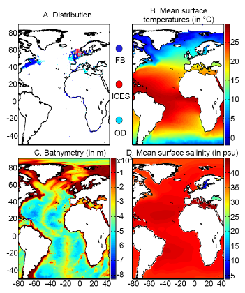
Figure 1 A. Spatial
distribution in the data of presence of a fish reported found in the databases
ICES, Fishbase or other smaller datasets (OD). B. Mean
observed sea surface temperature for the period 1960-2005. C.
Mean bathymetry in the Atlantic Ocean. D. Mean sea surface
salinity in the Atlantic Ocean.
Figure 1. Physical data
Our projections are based on three abiotic parameters:
bathymetry; salinity and sea surface temperature (use often as a proxy for
conditions at the larval stage).
Bathymetry data originated from a global ocean bathymetry map
(1 degree longitude x 1 degree latitude)(Smith & Sandwell 1997). This
dataset is among the most complete, high-resolution image of sea floor
topography currently available. The map was constructed from data obtained from
ships with detailed gravity anomaly information provided by the satellite
GEOSAT and ERS-1(Smith & Sandwell 1997). Bathymetry data were considered
because the spatial distribution of the Atlantic cod is in part explained by
this parameter as the species occurs mainly over continental shelves (Louisy
2002) (Fig. 1).
Annual Sea Surface Salinity (SSS, average values between 0 and
10 meters) data was obtained from the Levitus' climatology (Levitus 1982). ICES
data were used to complete the Levitus dataset in coastal regions where there
is no assessment of annual SSS (e.g. some regions of the eastern English
Channel). ICES data were downloaded from http://www.ices.dk. Salinity was
considered because it has a strong impact of the distribution of most fishes
(Fig. 1).
Sea Surface Temperature (SST) data originated from the
database International Comprehensive Ocean-Atmosphere Data Set (ICOADS,
longitudes with a spatial resolution of 1° longitude x 1° latitude;
http://icoads.noaa.gov)(Woodruff et al. 1987). An annual mean was calculated
for the period 1960-2005. Data on SST were considered as this parameter has
strong impact on the spatial distribution of cod (Brander 2000,
Intergovernmental Panel on Climate Change 2007) (Fig. 1).
All physical data were bilinearly interpolated on a spatial
grid of 0.1° longitude x 0.1° latitude at a global scale. While only
one map of bathymetry and SSS (annual climatology) was generated, a grid for
each year of the period 1960 to 2100 was built for SST (observed and
projected). Therefore, spatial distribution in the probability of presence of a
fish varies according to the three abiotic parameters while year-to-year
changes are only function of SST.
Mean values of bathymetry, sea surface temperature and
salinity are presented for the North Atlantic in Fig. 2.
Description of the Non-Parametric
Probabilistic Ecological Niche model (NPPEN)
The model is derived from a test recently applied to compare
the ecological niches (sensu (Hutchinson 1957)) of two species
(Beaugrand & Helaouët 2008). The analysis is based on Multiple
Response Permutation Procedures (MRPP), a test first proposed by Mielke et al.
(Mielke et al. 1981). MRPP has been applied in conjunction to Split Moving
Window Boundary analysis to detect discontinuities in time series (Cornelius
& Reynolds 1991). This method has also been utilised to identify abrupt
ecosystem shifts (Beaugrand 2004, Beaugrand & Ibanez 2004). Mathematically,
MRPP tests whether two groups of observations in a multivariate space are
significantly separated. (Mielke et al. 1981 gave a full description of the
test and Beaugrand & Helaouët {Beaugrand, 2008 #2205) have recently
illustrated the procedure in details in an adaptation of the technique to
compare two ecological niches.
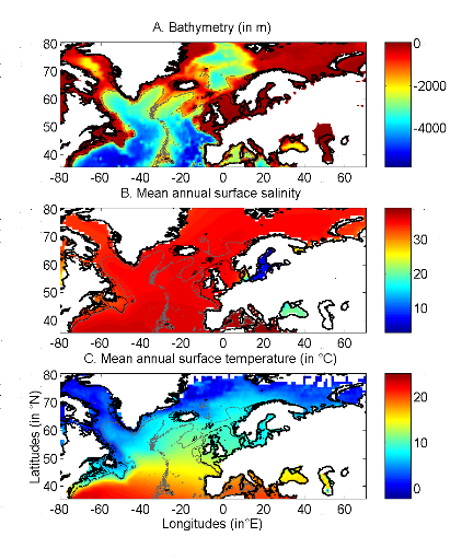
Figure 2 Spatial distribution of bathymetry (A), mean
annual sea surface salinity (B) and mean annual sea surface temperature (C) in
the North Atlantic Ocean. Isobaths 200m (dark grey line) and 2000m (light grey
line) are indicated.
The model we propose to assess the probability of occurrence
of cod (and its changes in space and time) is in fact a simplification of MRPP.
Instead of comparing two groups of observations, the analysis tests whether one
observation belongs to a group of (reference) observations we call here the
reference matrix. The reference matrix is represented by a matrix
Xn,p with n the number of (reference) observations
and p the number of variables. Each row of the matrix represents the
environmental conditions where a species was detected. It is crucial that the
reference matrix covers the entire niche (sensu Hutchinson) of a
species to give reliable probability (Thuiller et al. 2004). This point,
perhaps too often forgotten in this kind of exercise, was checked for each of
the 51 species used in this paper. The predictive matrix
Ym,p encompasses m observations of the environment
using also p predictors. Each observation of Y, encompassing
information on environmental conditions, will be tested against
X (range of conditions where the species was detected). The
model is applied in 4 main steps:
Step 1: homogenization of the reference
matrix
In contrast to the terrestrial realm where the presence of a
species can be more easily (visually) detected (at least for some species),
this is not so for many species in the pelagic realm and especially for fish.
The density of fish occurrence reported in the datasets depends on fishing
activities. It is clear that the density of data points is higher in fishing
area. Although this indicates to some extent that the resource is more abundant
in those regions, this is not completely true. This phenomenon can potentially
influence the outcome of any ecological niche model. Another phenomenon that
can influence the probability is the wrong report of data occurrence. This can
appear and it is not always possible to go through all individual observations.
Misreports can profoundly influence the probability. In an attempt to overcome
these drawbacks, we created a virtual cube (i.e. three controlling factors)
with intervals of sea surface temperature of 1°C between -2°C and
18°C, intervals of bathymetry of 20m between 0 and 800m and intervals of
salinity of 2 between 0 and 40 and retained one data occurrence when more than
one observation were detected in the crossed intervals of SST, bathymetry and
salinity. This threshold of two was fixed to eliminate the impact of one
misreport. The resolution could, at first sight, appear to be coarse. However,
the practice of the ecological niche model shows that the probability remains
similar, even at low resolution (see Fig. 4).
Step 2: preparation of data
A matrix called Zn+1,p is created
for each observation of Y to be tested against
X. For the first observation, the following matrix is
constructed:
 (1) (1)
With xi,j, the observations in matrix
X and yi,j, an observation of matrix
Y. The building of matrix Z is repeated m
times, corresponding to the m observations of Y.
Step 3: calculation of the mean multivariate
distance between the observation to be tested and the reference matrix
MRPP was first proposed to be applied with an Euclidean
distance, a squared Euclidean distance or a chord distance (Mielke et al.
1981). To first illustrate the technique, we use an Euclidean distance.
Obviously, if variables do not have the same unit or dimension, such a distance
should be avoided. The Euclidean distance is calculated as follows:
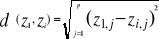 (2) (2)
With z1,j the first observations for the
jth variable originally the observation of the variable of matrix X,
1 = j = p; zi,j, the observation i of the variable j in matrix
Z with 2 = i = n+1 and 1 = j = p. Then, the average observed
distance åo is calculated as follows:
 (3) (3)
With n the total number of Euclidean distances, equal to the
number of observations in the training set X.
Step 4: calculation of the probability that
the observation belongs to the reference matrix
The mean Euclidean distance is tested by replacing each
observation of X by y in Z. The number of
maximal permutations is equal to n. After each permutation, the mean Euclidean
distance ås is recalculated, with 1 = s = n. A probability p
can be assessed by looking at the number of times a simulated mean Euclidean
distance is found to be superior or equal to the observed mean Euclidean
distance between the observation and the reference matrix X.
 (4) (4)
Where the probability p is the number of times the simulated
mean Euclidean distance was found superior or equal to the observed mean
distance. When p = 1, the observation has environmental conditions that
represent the centre of the species niche (sensu Hutchinson). When p =
0, the observation has environmental conditions outside the species niche. It
is essential to remind here that the niche and its borders have to be correctly
assessed. Applying the procedure to each observation of
Ym,p leads to a matrix Pm,1
of probability. It is important to have a large reference matrix so that
the resolution of the probability is as high as possible. The resolution R of
the probability is:
 (5) (5)
With n the number of reference observations in
X. Ideally, R should be < 0.05.
Simple example of application of the model using the
Euclidean distance
To illustrate the principle of the technique, we present a
hypothetical case where the reference matrix X has n = 3
observations and p = 2 controlling factors while the predictive matrix
Y has m = 1 observation (Fig. 3). Calculations of the three
Euclidean distances between y and the reference observations x give = 2.236, = 2.236,  = 2.236 and = 2.236 and  = 1.803. The average observed distance åo is = 2.092.
The simulated distances are ås1 = 1.589, ås2
= 1.383 and ås3 = 1.140. The probability is therefore equal to
0. Observation y has environmental conditions not compatible with the species
ecological niche inferred here from 2 variables. = 1.803. The average observed distance åo is = 2.092.
The simulated distances are ås1 = 1.589, ås2
= 1.383 and ås3 = 1.140. The probability is therefore equal to
0. Observation y has environmental conditions not compatible with the species
ecological niche inferred here from 2 variables.
Selection of a better coefficient of distance for Step
2
Mielke et al (1981) used mainly the Euclidean, squared
Euclidean and chord distances. However in the context of ecological niche
modeling, the use of the Euclidean (squared or not) distance in step 2 is not
appropriate in most (if any) cases. The chord distance can be used (Beaugrand
& Helaouët 2008). The computation of this distance is done by
normalizing each vector of Z to one prior to the calculation of the Euclidean
distances. The normalization is a special kind of scaling (Legendre &
Legendre 1998). Each element of the vector is divided by its length, using the
Pythagorean formula. This transformation ensured that each variable had the
same weight in the analysis. In our study, the normalization of elements of
Zn+1,p (see (1)) would be:
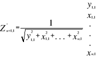 (6) (6)
Where x and y are as in (1). Here however, we prefer the use
of the Mahalanobis generalised distance that is independent of the scales of
the descriptors (as is the chord distance) but also takes into consideration
the covariance (or the correlation) among descriptors (Ibañez 1981). The
Mahalanobis generalised distance has been frequently used recently in this
context (e.g. (Calenge et al. 2008, Nogués-Bravo et al. 2008)). The
Prior to the calculation of the distance, standardisation of Z
is accomplished by the following transformation:
 (7) (7)
Where  are the observations i of the jth variables in
Z, are the observations i of the jth variables in
Z,  the average and the average and  the standard deviation of each variable j in Z. the standard deviation of each variable j in Z.
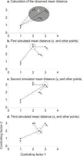
Figure 3 Principles of the calculation of the
niche model that lead to probability of occurrence of a species.
a. An hypothetical observation to be tested against a
training set (X) composed of three observations in the space of two controlling
factors. Three Euclidean distances are first calculated and then the average
observed distance between the observation to be tested and the ones of the
training set is assessed. b. Recalculation of the mean
distance after permutation of the first observation (x1) of the
training set by the observation to be tested. c. Recalculation
of the mean distance after permutation of the second (x2)
observation of the training set by the observation to be tested.
d. Recalculation of the mean distance after permutation of the
last observation (x3) of the training set X by the observation to be
tested. All calculated Euclidean distances are indicated by a dashed line. The
number of times the simulated mean distance is found inferior to the observed
mean distance defined the probability to find the species in a region.
To calculate the Mahalanobis generalized distance between each
observation of the environment yi (1 = i = m) and all observations
of the training set xj (1 = j = n), we used a particular form of the
generalized distance, giving the distance between any observation and the
centroid of an unique group (Dagnélie 1975):
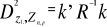 (8) (8)
With Rp,p the correlation matrix
of the standardized table (mean 0 and variance 1)
Z*, k1,p is the vector
of the differences between values of the p variables at  of standardized matrix Z* and the mean of standardized matrix Z* and the mean  of the p variables in the standardized matrix Z*. Therefore
in Step 3, the Euclidean distance was replaced by the use of the Mahalanobis
Generalised distance. Furthermore, comparison between the chord and the
Mahalanobis generalized distance shows that when correlation between two
parameters are significantly different to 0, the ecological niche model
performs better when it is based on the Mahalanobis generalized distance
(Fig. 4). of the p variables in the standardized matrix Z*. Therefore
in Step 3, the Euclidean distance was replaced by the use of the Mahalanobis
Generalised distance. Furthermore, comparison between the chord and the
Mahalanobis generalized distance shows that when correlation between two
parameters are significantly different to 0, the ecological niche model
performs better when it is based on the Mahalanobis generalized distance
(Fig. 4).
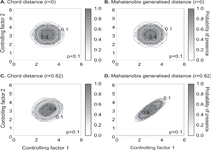
Figure 4 Fictive examples that show the better
performance of the Mahalanobis generalised distance in comparison to the chord
distance, justifying the choice of the distance coefficient in the ecological
niche model NPPEN. First, the reference matrix is composed of 25 observations
with two controlling factors. The correlation between the 2 controlling factors
is null (A and B). A.
Probabilities based on the chord distance (r = 0). B.
Probabilities based on the Mahalanobis generalised distance (r = 0). Second,
the reference matrix is composed of 13 observations with 2 parameters. The
correlation between the two controlling factors is high (r = 0.82;
C and D). C. Probabilities
based on the chord distance (r = 0.82). D. Probabilities based
on the Mahalanobis generalised distance (r = 0.82). Black circles denote the
reference observations (reference matrix). High probabilities are located at
the centre of the reference matrix, denoting the centre of the ecological niche
(sensu Hutchinson) and probabilities <0.1 are situated outside
(white colour).
Maps of probability of presence are then assessed from the
knowledge of the three abiotic factors and by linear interpolation in the space
of the ecological niche. Figure 5 presents the modelled
ecological niche for Cod (Gadus morhua L.).
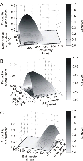
Figure 5 Realised niche (sensu
Hutchinson) of the Atlantic cod. A. Probability of cod
occurrence as a function of bathymetry and mean annual sea surface temperature.
B. Probability of cod occurrence as a function of mean annual
sea surface salinity and mean annual sea surface temperature.
C. Probability of cod occurrence as a function of mean annual
sea surface salinity and bathymetry.
Description of the climatic atlas
It was possible to apply the technique on 51 species of
commercially exploited marine species (see Species Summary pages 15 and 16)
The attempt to use the model on other species was not
satisfactory because of a lack of occurrence data or a too incomplete coverage
of the ecological niche. A confidence index was set up and used on each map in
a first attempt to assess the robustness of projections. The values of the
index were based on the number of presence data on which the model was applied.
The index was expressed in four categories. A value of 1, 2, 3, 4 means that
the model was applied on <100, 200-500, 500-1000, >1000 occurrence data,
respectively. Projections are likely to be more reliable for an index of 4
(e.g. the Atlantic cod).
For each of the 51 species, nine figures are attached. The
first figure shows the spatial distribution of presence data used to apply the
ecological niche model (Fig. 6). The total number of samples
on which the model is utilised is indicated on the left of the figure
(Fig. 6).
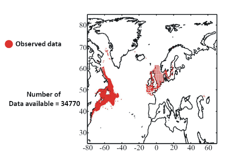
Figure 6 Spatial distribution of occurrence
data for the Atlantic cod.
Other maps (from two to nine) present modelled probability of
presence (between 0 and 1) for the decades 1960s (observed data), 2000s, 2010s,
2020s, 2030s, 2040s, 2050s and 2090s (scenario B2). A null probability means
that the physical conditions are incompatible with the presence of the species
while a probability of 1 means that the presence of the species is certain.
Figure 7 shows an example for the Atlantic cod (1960s).
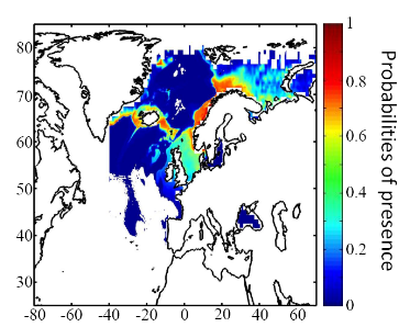
Figure 7 Spatial distribution in the
probability of presence for the Atlantic cod for the period 1960-1969.
Conclusions
The documents present a first outline on the potential changes
in the spatial distribution of 51 commercially exploited species up to 2100
using a moderate scenario (Scenario B2, ECHAM 4). It is the result of an
investigation of the relationships between climate and marine resources. Future
developments should include a multimodel and a multiscenario approach to attach
a better confidence interval on the projections. Two scientific papers are in
preparation for submission. The delay in submitting the two papers is explained
by a methodological development in 2008. The originally double approach using a
parametric and a non-parametric technique has been replaced by a new technique
combining strength of the two procedures: the use of the Mahalanobis technique
and its test by a non-parametric procedure called MRPP and published in 2008
(Beaugrand et Helaouët 2008, Marine Ecology Progress Series; volume 363;
pages 29-37). The two papers will be soon submitted in good scientific journals
and are provisionally entitled:
· Beaugrand G, Lenoir S, Ibañez F, Manté C
(submit) Modelling the probability of occurrence of the Atlantic cod.
· Lenoir S, Beaugrand G, Lécuyer E. (submit)
Modelled spatial distribution of marine fish and projected modifications in the
North Atlantic Ocean.
References
Beaugrand G (2004) The North Sea regime shift: evidence,
causes, mechanisms and consequences. Progress in Oceanography 60:245-262
Beaugrand G, Helaouët P (2008) Simple procedures to
assess and compare the ecological niche of species. Marine Ecology Progress
Series 363:29-37
Beaugrand G, Ibanez F (2004) Monitoring marine plankton
ecosystems (2): long-term changes in North Sea calanoid copepods in relation to
hydro-meteorological variability. Marine Ecology Progress Series 284:35-47
Brander K (2000) Effects of environmental variability on
growth and recruitment in cod (Gadus morhua) using a comparative approach.
Oceanologica Acta 23:485-496
Calenge C, Darmon G, Basille M, Loison A, Jullien J-M (2008)
The factorial decomposition of the Mahalanobis distances in habitat selection
studies. Ecology 89:555-566
Cornelius JM, Reynolds JF (1991) On determining the
statistical significance of discontinuities within ordered ecological data.
Ecology 72:2057-2070
Dagnélie P (1975) Theorie et methodes statistiques,
Applications agronomiques. . In: Les methodes de l'inférence statistique
2e ed, Vol 2. Presses agronomiques de Gembloux, Gembloux, p 463
Hutchinson GE (1957) Concluding remarks. Cold Spring Harbor
Symposium Quantitative Biology 22:415-427
Ibañez F (1981) Immediate detection of heterogeneities
in continuous multivariate, oceanographic recordings. Application to time
series analysis of changes in the bay of Villefranche sur Mer. Limnology and
Oceanography 26:336-349
Intergovernmental Panel on Climate Change WGI (2007) Climate
Change 2007: Impacts, Adaptation and Vulnerability, Vol. Cambridge University
Press, Cambridge
Legendre P, Legendre L (1998) Numerical Ecology, Vol. Elsevier
Science B.V., The Netherlands
Levitus S (1982) Climatological Atlas of the World Ocean. In:
office USGp (ed) NOAA ProfPap, Vol 13, Washington DC, p 173
Louisy P (2002) Guide d'identification des poissons marin:
Europe et Méditerranée, Vol, Milan
Mielke PW, Berry KJ, Brier GW (1981) Application of
Multi-Response Permutation Procedures for examining Seasonal changes in monthly
mean Sea-Level pressure patterns. Monthly Weather Rewiew 109:120-126
Nogués-Bravo D, Rodriguez J, Hortal J, Batra P, Araujo
MB (2008) Climate Change, Humans, and the Extinction of the Woolly Mammoth.
PLoS Biology 6:685-692
Smith WHF, Sandwell DT (1997) Global Sea Floor Topography from
Satellite Altimetry and Ship Depth Soundings. Science 277:1956-1962
Thuiller W, Brotons L, Arau' jo MB, Lavorel S (2004) Effects
of restricting environmental range of data to project current and future
species distributions. Ecography 27:165-172
Woodruff S, Slutz R, Jenne R, Steurer P (1987) A comprehensive
ocean-atmosphere dataset. Bulletin of the American meteorology society
68:1239-1250

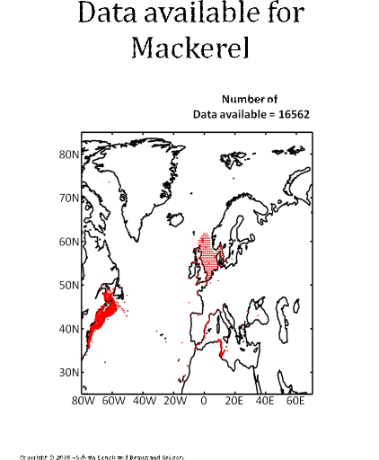
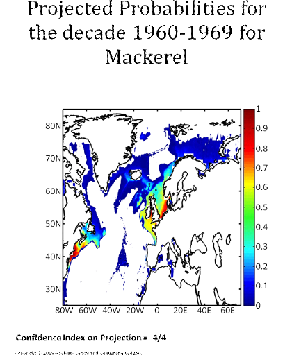


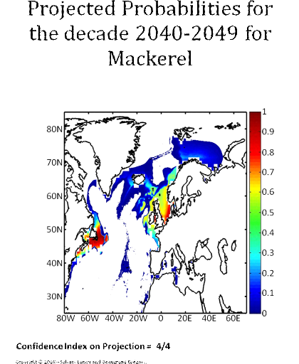
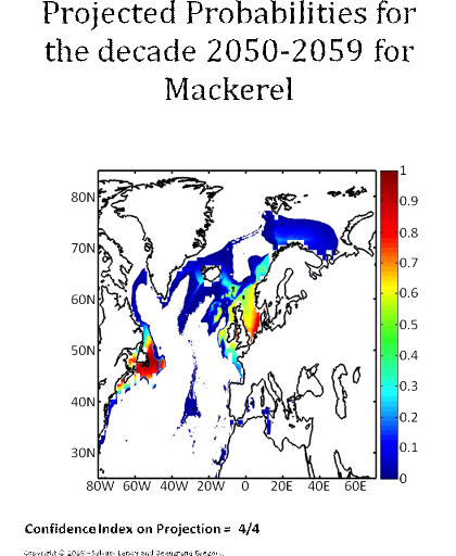
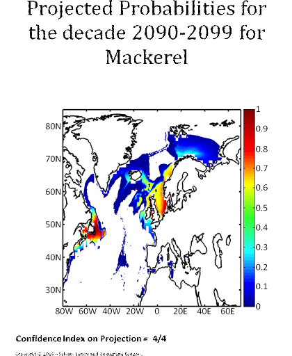
CHAPITRE IV
Les effets du climat sur les proies principales des
oiseaux marins en mer du Nord
1. Résumé du
Chapitre IV
1.1. Avant-propos
L'écosystème mer du Nord connait depuis les
années 1980 de profonds et rapides changements dans sa trophodynamique
(Kirby & Beaugrand, 2009) Ces changements, provoqués par le
réchauffement climatique, atteignent la phénologie (Edward &
Richardson, 2004) et la biogéographie des espèces
résidentes (Stebbing et al., 2004 ; Genner et
al., 2004 ; Perry et al., 2005). Les effets du
réchauffement concernent l'ensemble du réseau trophique tout au
long duquel ces effets se répercutent (Frederiksen et al.,
2004 ; Kirby & Beaugrand, 2009). Au sommet du réseau trophique,
les prédateurs supérieurs sont considérés comme des
indicateurs de l'état de l'écosystème marin (Wanless,
2007). Parmi eux, les oiseaux marins nichant sur les côtes de la mer du
Nord, types Alcidés et Laridés, ont connu récemment des
chutes importantes de leur taux de reproduction. Ces baisses sont liées
à des modifications dans la qualité et la disponibilité
des proies préférentielles, en particulier le lançon
nordique (Wanless et al., 2007). Cette raréfaction du
lançon nordique est accompagnée par une augmentation d'abondance
d'autres poissons à valeur énergétique bien plus faible
comme l'entélure (Wanless et al., 2005, 2007). Cette
réorganisation de la composition spécifique du régime
alimentaire des oiseaux marins est imputable au réchauffement des eaux
de la mer du Nord (Harris et al., 2007, 2008). Les conditions de vie
de cette zone deviendront moins favorables à la présence du
lançon nordique. En revanche, elles favoriseront d'autres espèces
aux exigences environnementales plus en adéquation avec ces conditions
de vie, nouvellement disponibles.
Dans cette étude, les distributions spatiales
passées, présentes et futures potentielles des espèces de
poissons disponibles et capturées par les oiseaux marins, tels que le
Guillemot de Troïl ou la mouette tridactyle, ont été
modélisées grâce au NPPEN. Ces espèces sont le
lançon nordique (Ammodytes marinus Raitt, 1934), le sprat
européen, (Sprattus sprattus Linnaeus, 1758) et
l'entélure (Entelurus aequoreus Linnaeus, 1758). La possible
immigration en mer du Nord de deux autres espèces, plus
méditerranéennes, l'anchois (Engraulis encrasilocus
Walbaum, 1792) et la sardine européenne (Sardina pilchardus
Linnaeus, 1758) a également été évaluée.
L'objectif était d'estimer si la substitution de proies à haute
valeur énergétique par des espèces de bien plus faible
qualité, observée dans le régime alimentaire des oiseaux
marins de mer du Nord, allait perdurer avec le réchauffement climatique.
Un second objectif consistait à évaluer si les espèces,
à la distribution spatiale généralement située plus
au sud, et dont l'arrivée en mer du Nord est prédite, peuvent
constituer une ressource de substitutions valable pour les oiseaux marins.
1.2. Données
utilisées
? Données biotiques
Trois espèces de poissons ont été
choisies pour leur importance en terme de ressource alimentaire et de nombre de
captures pour les oiseaux marins de la mer du Nord : le lançon
nordique (Ammodytes marinus Raitt, 1934), le sprat européen
(Sprattus sprattus Linnaeus, 1758) et l'Entélure (Entelurus
aequoreus Linnaeus, 1758). Deux autres espèces, à la
distribution plus méditerranéenne ou subtropicale, et
également source de nourriture pour les oiseaux marins dans ces
régions, ont été ajoutées : la sardine
européenne (Sardina pilchardus Walbaum, 1792) et l'anchois
européen (Engraulis encrasilocus Linnaeus, 1758).
Excepté pour la sardine européenne, les
données de présence de ces espèces ont été
récupérées, comme pour les précédents
chapitres, à partir de la base de données en ligne FishBase
(Froese & Pauly, 2009) complétée avec des données
provenant, du Conseil International pour l'Exploitation de la Mer (CIEM, 2005b,
2007), de la littérature et des connaissances scientifiques sur la
distribution spatiale de ces espèces. Ces observations sont
datées et géo-référencées. En ce qui
concerne la sardine européenne, le manque de données
d'observation exploitables, nous a conduits à définir la niche
écologique de cette espèce à partir de sa distribution
connue. La sardine européenne a été
considérée comme se répartissant le long du golfe de
Gascogne, entre la mer Celtique et le sud de la mer du Nord au nord, et les
eaux nord-africaines (côtes de la Mauritanie) au sud, en incluant la mer
Méditerranée.
? Données abiotiques
Les paramètres physiques qui ont été
utilisés sont : la température de surface (SST), la
bathymétrie et la salinité de surface (SSS). De plus, un
troisième descripteur environnemental, la nature sédimentaire du
fond, a été utilisé pour le lançon nordique qui
passe une partie de son temps de vie (la nuit et la période hivernale)
enfoui dans le sédiment.
Les données de bathymétrie et de SSS proviennent
des mêmes sources que celles utilisées dans les chapitres II et
III. Par contre, les données de SST inclues pour modéliser la
distribution spatiale passée et présente des espèces sont
issues d'une base de données ICOADS mise à jour : les
données SST couvrent dorénavant la période de 1960
à 2008. Les SST utilisées pour prédire la
répartition potentielle des espèces dans le futur sont celles des
scénarios SRES A2 et B2 du modèle ECHAM4 pour la période
de 1990 à 2100. Les informations concernant la nature du sédiment
proviennent du « Service Hydrogéographique et
Océanographique de la Marine » (SHOM, Fig. IV.S1).
La zone géographique couverte par les variables
environnementales s'étend des latitudes 25°N à 85°N et
des longitudes 80°O à 65°E. Les valeurs des variables sont
interpolées de façon bilinéaire avec une résolution
de 0,1° de latitude et de longitude. L'étude de l'évolution
annuelle des probabilités de présence des espèces s'est
focalisée sur la mer du Nord (zone CIEM IV), délimitée par
les longitudes 4°O et 9°E et par les latitudes 51°N et
62°N.
1.3. Méthode et
Analyses effectuées
? Méthode
Les méthodes utilisées, le NPPEN et
l'homogénéisation, ont été décrites dans les
sections précédentes.
? Analyse 1
À partir des données brutes d'observation et
après homogénéisation pour le lançon nordique, le
sprat européen, l'entélure et l'anchois européen, les
préférendums environnementaux ont été
évalués pour chacun des paramètres
(préférendums thermiques : Fig. IV.1 ;
préférendums de salinité : Fig. IV.S2 ; les
différents préférendums bathymétriques n'ont pas
été représentés).
? Analyse 2
Deux procédures de validation des résultats
produits par le modèle ont été menées. Une
première consistait à utiliser le modèle avec seulement
50% des données d'observations puis à comparer les
résultats obtenus (corrélation en rang de Spearman) avec les 50%
des données d'observation restantes, pour le lançon nordique, le
sprat européen et l'entélure (Fig. IV.S3). Le peu de
données disponibles pour la sardine et l'anchois européens n'a
pas permis d'effectuer cette étape de validation sur ces espèces.
La deuxième procédure visait à comparer l'évolution
annuelle, en zone CIEM IV, de la biomasse des reproducteurs (SSB) du
lançon nordique, aux probabilités annuelles de présence
calculées par le NPPEN dans cette zone, de 1983 à 2006 (Fig.
IV.S4).
? Analyse 3
Le modèle NPPEN a été utilisé pour
cartographier la distribution spatiale de chacune des espèces pour les
périodes 1960-1969, 2000-2008 puis 2050-2059 et 2090-2099
scénarios SRES A2 et B2 (Fig. IV.2 et Figs. IV.S5 à IV.S9). Puis,
les probabilités de présence annuelles de chacune des
espèces ont été calculées en mer du Nord (Fig.
IV.3).
1.4. Principaux
résultats obtenus
? Analyse 1
L'étude des préférendums thermiques a
permis de mettre en évidence les différences entre les
espèces sélectionnées en fonction de leurs limites et leur
domaine de tolérance thermiques (Fig. IV.1). La niche thermique a
été estimée entre 8 et 12°C pour le lançon
nordique, entre 7 et 17°C pour le sprat européen, entre 7 et
14°C pour l'entélure, entre 9 et 28°C pour l'anchois
européen et entre 13 et 23°C pour la sardine européenne.
Toutes les espèces affichent des préférendums de
salinité compris entre 30 et 35, mis à part le sprat
européen qui est une espèce présente en mer Baltique.
? Analyse 2
Les données de présence observées, pour
le lançon nordique, le sprat européen et l'entélure
apparaissent, en majorité, là où les probabilités
modélisées de présence de l'espèce sont grandes
(Fig. IV.S3). L'évolution annuelle passée des SSB du
lançon nordique et les probabilités produites par le NPPEN sont
corrélées avec un r = 0,63 (p<0,001).
? Analyse 3
Les cartes de distribution potentielle, basées sur les
périodes 1960-1969 et 2000-2008 (Fig. IV.2), associées à
l'évolution annuelle des probabilités de présence (Fig.
IV.3) illustrent les changements dans la disponibilité de la proie
préférée des oiseaux marins : le lançon
nordique. Le modèle décrit, également, une augmentation
réellement observée de l'entélure, espèce
représentant une ressource alternative de piètre qualité
pour les oiseaux. Dans le futur, le sprat européen et l'entélure
verront leur population se maintenir jusqu'au milieu du siècle, pour
décliner par la suite. Le lançon nordique verra sa population
disparaître petit à petit de la mer du Nord. Enfin, si l'anchois
européen semble pouvoir coloniser le sud de la mer du Nord, la sardine
européenne semble ne jamais pouvoir s'y établir (Figs. IV.2 et
IV.3).
1.5. Conclusion
Les résultats du modèle NPPEN confirment bien
les changements, déjà observés, dans la
disponibilité des proies des oiseaux marins de la mer du Nord. Le
lançon nordique, ressource très prisée, possède une
niche thermique centrée sur 10°C. Le réchauffement des eaux
de la mer du Nord rend cette zone défavorable à sa survie. Les
limites de la niche thermique de cette espèce ne lui permettent pas de
conserver des populations aussi abondantes que celles qu'elle a connues dans
une mer du Nord plus froide. Le sprat européen et l'entélure ont
une niche centrée vers 12°C et aux limites supérieures bien
plus importantes de celles du lançon nordique. Ainsi, le
réchauffement climatique a permis à ces deux espèces de
voir leurs populations augmenter par le passé, et leur permettra de
conserver les mêmes niveaux d'abondances jusqu'au milieu du
siècle. Par la suite, les températures de la mer du Nord se
réchaufferont au point de sortir des limites des
préférendums thermiques du sprat européen et de
l'entélure.
Cette réorganisation spatiale des poissons à
disposition des oiseaux marins, en mer du Nord, a donc pu induire, ou tout au
moins participer, à la chute du succès de reproduction de ces
oiseaux. En effet, le lançon nordique disparaissant en raison du
réchauffement des eaux et de la mer du Nord associée à une
pression de pêche importante, l'entélure bien que de piètre
qualité énergétique, constitue une alternative de
pêche. Toutefois, la quantité d'énergie nécessaire
à la reproduction des oiseaux est, dans le cas d'un régime
composé d'une grande quantité d'entélure, beaucoup plus
difficilement atteinte. Dans le futur, la sardine et l'anchois
européens, proies valables pour les oiseaux en
Méditerranée et sur les côtes atlantiques
françaises, ne pourront remplacer le lançon nordique dans le
régime alimentaire des oiseaux en mer du Nord. La sardine
européenne ne trouvera jamais de conditions satisfaisantes pour
s'établir en mer du Nord et les populations d'anchois européen,
n'atteindront pas un niveau d'abondance suffisant avant la fin du
siècle.
.
2. Publication: The effect
of climate on the main fish prey of North Sea seabirds
The effect of climate on the main fish prey of North
Sea seabirds
Short title: Climate effects on main seabird
prey
S. Lenoir, G. Beaugrand, M. Jaffré, R. R. Kirby
Proceeding of the Royal society of London B
(submitted)
2.1. Abstract
Climate change has been a source of major alteration of the
trophodynamics of the North Sea ecosystem since the 1960s. One manifestation of
change has been a decline in seabird breeding success due to climate-induced
changes in their preferred fish prey of lesser sandeels (Ammodytes
marinus) and European sprat (Sprattus sprattus), together with a
recent increase in the abundance of snake pipefish (Entelurus
aequoreus), which is a poor food for seabirds. Here, we apply an
ecological-niche model comprising four environmental variables (sea surface
temperature, bathymetry, salinity, sea bottom sediment type) to model changes
in the abundance of these three fish in the North Sea to the end of the
21st century, and to determine whether a climate-induced change in
their abundance will be compensated by the appearance of the European sardine
and anchovy in the North Sea, two warmer water southern fish species. Our
analyses indicate that a decrease in the abundance of the lesser sandeel
observed at the end of the 1980s and the 1990s will intensify towards the
middle and the end of the 21st century and the sprat will show a
severe decline from 2050-2100; these changes are likely to further compromise
seabird breeding success in the North Sea. Furthermore, our model suggests that
it is unlikely that either the European sardine (Sardina pilchardus)
or the European anchovy (Engraulis encrasicolus), which might be
consumed by some seabirds, will counteract the changes in abundance of their
current preferred pelagic fish prey.
Keywords: climate change, ecological-niche
model, fish, seabirds, sea surface temperature
2.2. Introduction
Climate warming has become unequivocal (Intergovernmental
Panel on Climate Change 2007b) and over the last 40 years the ocean has
absorbed 84% of the heat added to the climate system (Levitus et al.
2005). Several significant correlations between changes in climate and in the
abundance of marine species, ranging from plankton to fish and seabirds
(Aebischer et al. 1990; Beaugrand & Reid 2003; Frederiksen et
al. 2006), suggest that marine ecosystems have responded quickly to a
warming of temperature (Richardson & Shoeman 2004; Beaugrand et
al. 2009; Drinkwater et al. 2010). For example, a sustained
climate-induced change occurred in the trophodynamics of the North Sea
ecosystem during the 1980s (Kirby et al. 2009) that altered the
phenology (Edwards & Richardson 2004) and the biogeography of many species
(Stebbing et al. 2002; Genner et al. 2004; Perry et
al. 2005) across several trophic levels (Frederiksen et al. 2004;
Kirby & Beaugrand 2009), and including the breeding success of seabirds
such as black-legged kittiwakes and common guillemots (Wanless et al.
2005 ; Harris et al. 2007; Harris et al. 2008).
North Sea seabird breeding success appears to be controlled
partially by the abundance (Poloczanska et al. 2004; Frederiksen
et al. 2005), distribution (Shealer 2002; Grémillet &
Boulinier 2009) composition and nutritional quality of the prey the parent
birds feed to their chicks on the nest (Wanless et al. 2005; Harris
et al. 2008). As a consequence, an observed reduction in the breeding
success of some North Sea seabird colonies has been attributed to dietary
changes (Wanless et al. 2005; Harris et al. 2008). In
particular, three species of fish in the North Sea, the lesser sandeel
(Ammodytes marinus), the European sprat (Sprattus
sprattus) and the snake pipefish (Entelurus aequoreus) seem
to be important determinants of North Sea seabird breeding success (Harris
et al. 2007, Harris et al. 2008); While the lesser sandeel
and the European sprat, which are high energy fish, are the preferred prey, the
snake pipefish, although frequently recorded in the diet of seabirds since
2004, and found discarded at nest sites, is a poor food for young chicks
(Harris et al. 2008). Changes in the abundance and nutritional value
of lesser sandeels and sprats, and in the abundance of snake pipefish, due to a
combination of overfishing and the effects of hydroclimatic change (Frederiksen
et al. 2004) seem to have acted synergistically to compromise North
Sea seabird breeding success recently (Wanless et al. 2005; Wanless
2007).
To further explore the possible effect of hydroclimatic change
on the North Sea ecosystem with regard to the main fish prey of North Sea
seabirds we applied a recently developed ecological niche model to forecast
past and future spatial changes in the probability of occurrence of North Sea
sandeels, sprats, and snake pipefish(Beaugrand et al in press; Lenoir et al in
press). We took into account sea surface temperature (SST), bathymetry, sea
surface salinity (SSS) (see electronic supplementary material, figure IV.S1),
and, in the case of sandeels, bottom-sediment type (figure IV.S2). We then
applied our model to determine whether future changes in the hydroclimatic
regime of the North Sea may lead to a future increase in the abundance of two
warm-water southern fish species, the European sardine (Sardina
pilchardus) and the European anchovy (Engraulis encrasicolus). In
a similar way to which climate altered the dietary composition of common
guillemots (Uria aalge) in the California Current (Veit et
al. 1996; Oedekoven et al. 2001), an increase in the abundance of
sardine and anchovy in the North Sea could potentially compensate any decrease
in the abundance of North Sea sprats and sandeels.
2.3. Material and
Method
? Biological data
Sandeel, European sprat, snake pipefish, European anchovies
and European sardine data (post-larval stages) were obtained from the Ocean
Biogeographic Information System (OBIS; available at:
http://www.iobis.org/), the Global
Information Biodiversity Service (GBIF; available at:
http://data.gbif.org/), and the
ICES-FishMap online atlas (available at:
http://www.ices.dk/marineworld/fishmap/ices/).
Both temporal and spatial data are available for the majority of occurrences
with the exception of the sardine where, due to reduced spatial coverage, we
determined the current spatial range based upon expert knowledge and
examination of the OBIS data. First, we determined the minimum and maximum
latitudinal occurrence of the sardine by examining the OBIS data. Second, we
completed the occurrence point between 20°N and 54°N in each node of
a spatial grid of 0.1° longitude x 0.1° latitude where bathymetry was
between 0 and 3000m (North Atlantic, including the Mediterranean Sea and the
North Sea).
? Environmental data
Mean annual SST for the period 1960-2008 were obtained from
the International Comprehensive Ocean-Atmosphere Data Set (ICOADS,
http://icoads.noaa.gov; Woodruff
et al. 1987) and from the ECHAM 4 model (EC for European Centre and
HAM for Hamburg; for modelled SST data based upon climate change scenarios A2
(scenario of a divided world) and B2 (scenario of a divided world, but more
ecologically friendly; Intergovernmental Panel on Climate Change 2007b). The
SST data are therefore modelled data based on scenario A2 (a concentration of
carbon dioxide of 856 ppm by 2100, which represents an increase of
CO2 similar to that currently observed) and B2 (a concentration of
carbon dioxide of 621 ppm by 2100) and they reflect world populations of 15.1
and 10.4 billion people in 2100, respectively (Intergovernmental Panel on
Climate Change 2007b). For comparison purposes SST were also averaged for the
decades, 1960-1969, 2050-2059 and 2090-2099, and for the period 2000-2008.
In addition to hydroclimatic change, other physical habitat
variables that influence the distribution of fish species are sea surface
salinity (SSS) (electronic supplementary material, figure IV.S1)
(Schmidt-Nielsen 1990) and bathymetry (Louisy 2002), and, for species such as
the sandeel that has a benthic phase, the bottom-sediment type. We obtained
data for mean annual SSS from both Levitus' climatology (Levitus 1982) and ICES
(
http://www.ices.dk; Lenoir et
al. 2010); we did not include temporal changes in SSS for two reasons,
firstly, spatial variance in salinity is much more pronounced than the temporal
variance and secondly, temporal variance is poorly assessed in the
Atmosphere-Ocean General Circulation (AO-GCM) models (Martin Visbeck, Personal
Communication). We obtained bathymetry data from the global ocean bathymetry
map (Smith & Sandwell 1997) and for the sandeel we obtained data on
bottom-sediment type from the "Service Hydrogéographique et
Océanographique de la Marine" (SHOM). (electronic supplementary
material, figure IV.S2).
? Calculation of thermal niches
We used occurrence data to assess the thermal niche
(sensu Hutchinson, Hutchinson 1957) of each species by calculating the
number of individuals recorded per degree of annual SST (figure IV.1).
? Mapping of species occurrence
We used the non-parametric probabilistic ecological niche
model (NPPEN; Beaugrand et al. in press; Lenoir et al. 2010,
and electronic supplementary material 1), to assess the probability of species
occurrence and to map their potential spatial distribution. Briefly, the
technique tests whether environmental conditions within a cell in a
geographical space belong to the estimated ecological niche of a species. The
model tests whether or not an observation (i.e. the j geographical cells of our
environmental grids), characterised by an environmental stratum (p variables),
belongs to a reference matrix, here matrix Zm,p.
Mathematically, the technique is nonparametric using a modified version of the
multiple response permutation procedure (MRPP; Mielke et al. 1981).
The technique uses the Generalised Mahalanobis distance
(Mahalanobis, 1936), which enables the correlation between variables to be
considered (Farber & Kadmon 2003). The distance was calculated as
follows:
 (1) (1)
With x the vector of length p, representing
the values of the three/four environmental stratums to be tested
(j=2,530,206), Rp,p the correlation matrix of
reference matrix Zm,p and  the average environmental condition inferred from
Zm,p. The significance of the Generalised
Mahalanobis distance was then assessed using a simplified version of the MRPP
(Beaugrand et al. in press; Lenoir et al. 2010). the average environmental condition inferred from
Zm,p. The significance of the Generalised
Mahalanobis distance was then assessed using a simplified version of the MRPP
(Beaugrand et al. in press; Lenoir et al. 2010).
? Long-term changes in the probability of fish
occurrence
Long-term spatial changes in the probability of fish
occurrence were calculated for the five species on an annual basis from 1960 to
2100. Maps of species occurrence were built for the period 1960-1969,
2000-2008, 2050-2059 and 2090-2099 within the North Sea spatial domain ranging
from 4°W to 9°E and from 51°N to 62°N (figures IV.2?IV.3;
electronic supplementary material, figures IV.S3?IV.S7).
? Validation of the model
We used correlation analysis (Spearman's rank correlation) to
validate the modelled spatial distributions of each fish species by comparing
the probabilities of occurrence modelled by NPPEN with the percentage of the
number of actual presence data points in the North Sea for 2000-2008 (figure
IV.4). Only half of the data, not incorporated to the model, were used for
validation. We also use correlation analysis to compare the long-term changes
in spawning stock biomass (SSB) of the lesser sandeel (two-year old fish) to
the annual average probabilities of occurrence modelled by NPPEN in the ICES
subarea IV for the period 1983-2003 (figure IV.5). No SSB data were available
for the four other species in this area.
2.4. Results
Figure IV.1 shows the thermal niche of lesser sandeel, sprat,
snake pipefish, European anchovy and European sardine superimposed upon the
mean annual thermal regime of the North Sea for the four time periods we
considered. The thermal niches of the snake pipefish and the sprat range
between 7 to 14°C and 7 to 17, respectively. In contrast, the lesser
sandeel has a colder and narrower thermal niche between 8 and 12°C. The
warmer thermal niches of the European anchovy and European sardine lie between
9 and 28°C and 13 and 23°C, respectively. Our results suggest that
the thermal regime of the North Sea may soon exceed the thermal niche of the
lesser sandeel (figure IV.1a) and may become too warm for the snake
pipefish during the second half of the century under both scenarios A2 and B2
(figure IV.1c). In contrast, while the thermal niche of sprat
continues to match the thermal regime of the North Sea throughout the
21st century, the warming of the North Sea may lead to a reduction
in their probability of occurrence (figure IV.1b). Interestingly, the
extent of North Sea warming appears to be insufficient to lead to a significant
increase in abundance of either the European anchovy or the European sardine by
the end of the 21st century (figure IV.1d,e).
The long-term changing spatial probabilities of fish
occurrence modelled by NPPEN for the periods 1960-1969, 2000-2008, 2050-2059
and 2090-2099 (Scenario B2) revealed a northward movement of all species by
2090-2099 (figure IV.2). In the North Sea, the probability of occurrence of
lesser sandeel decreases progressively from the 1960s onwards and, while the
model predicts a transient increase in the probability of occurrence of sprat
and snake pipefish around the beginning of the 21st century, both
sprat and snake pipefish show a decline in abundance after 2050 in the central
North Sea, although the probability of sprat occurrence remains moderate along
northern Scottish coasts. With respect to changes in the probability of
occurrence of the two warm water southern fish species, we found that neither
species achieve a high level of abundance during the modelled period. The
European sardine appears to not increase in its probability of occurrence in
the North Sea even by the end of the 21st century, despite an increase along
the European shelf-edge, and while the probability of occurrence of anchovy in
the North Sea is predicted to increase by the middle of this century, the
increase is only moderate (figure IV.2). We found similar results when Scenario
A2 was utilised (figures IV.S3?IV.S7).
Figure IV.1 : Estimated thermal niche for
(a) lesser sandeel, (b) European sprat,
(c) snake pipefish, European anchovy (d) and
European sardine (e). Mean SST for the North Sea were added
for time periods 1960-1969, 2000-2008 and both A2 and B2 scenarios for the time
periods 2050-2059 and 2090-2099.
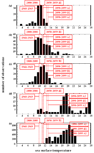
The examination of the long-term change in the probability of
fish occurrence in the North Sea revealed a strong increase in two phases at
the end of the 1980s and the 1990s for snake pipefish, sprat, and a pronounced
decrease in the probability of occurrence of lesser sandeel at the end of the
1990s (figure IV.3a). The probability of the occurrence of European
anchovy increased slightly at the end of the 1980s. No alteration in the
probability of sardine occurrence was detected for the period 1960-2008. When
we applied the same model to the period 2009-2100 we found that the occurrence
probability of lesser sandeel decreased steadily from 1990 to 2100 (figure
IV.3b). In contrast, the probability of occurrence of sprat and snake
pipefish levelled off during the first half of the century, following an
initial increase at the beginning of the century, to be followed by a decline
in their probability of occurrence from 2050 to 2100. The probability of
occurrence of the European anchovy increased from 0.18 at the beginning of the
21st century to 0.40 by its end (figure IV.3b). The
European sardine would not reach value of 0.05 in occurrence probability before
the end of the century.
We found a strong correlation (ranging from r=0.80 to r=0.83)
between the observed and modelled occurrence for lesser sandeel, sprat and
snake pipefish in the North Sea (figure IV.4); the coefficient of correlation
ranged from r=0.80 to r=0.83. Our comparison between temporal changes in
Spawning Stock Biomass (SSB) of the lesser sandeel (1981-2006) and modelled
data also revealed a strong correlation between the long-term changes in SSB
and the probability of occurrence modelled by NPPEN (figure IV.5).
Unfortunately, it was impossible to provide a similar comparative analysis for
the European anchovy or the European sardine due to the very low abundance of
these species in the North Sea during our study period
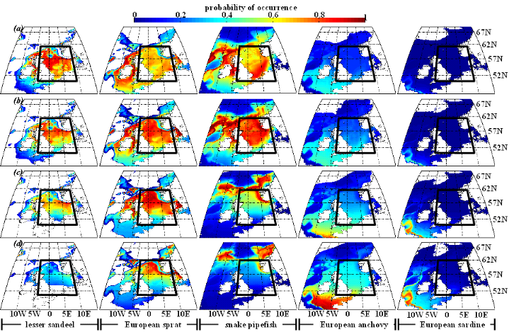
Figure IV.2 : Estimated probability of
occurrence using NPPEN for the time periods 1960-1969 (a),
2000-2008 (b), 2050-2059 (c) and 2090-2099
using scenario B2 (d) for, from left to right: lesser sandeel,
European sprat, snake pipefish, European anchovy and European sardine.


Figure IV.3 : Long-term changes in the annual
mean of the probability of occurrence in the North Sea (bounding box), for
snake pipefish (black lines), European sprat (red lines), lesser sandeel (blue
lines), European anchovy (green lines) and European sardine (cyan lines) from
1960 to 2008 (a) based on ICOADS temperature database and from
2009 to 2100 (b) based on ECHAM4 temperature scenarios (solid
line for scenario A2 and dashed line for scenario B2).
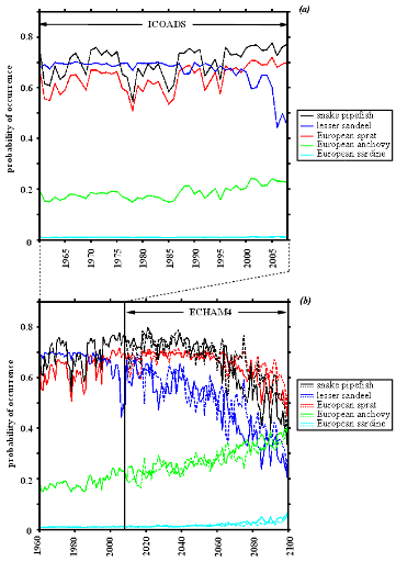
2.5. Discussion
Small planktivorous fish such as sandeel, sprat, anchovy and
sardine are an important trophic group in marine ecosystems where they
facilitate the transfer of energy from lower trophic levels, the plankton, to
higher trophic levels such as large predatory fish and seabirds. Our analysis
of sandeels and sprats in the North Sea from 1960 to the end of the
21st century suggests that a continued warming of the North Sea will
cause the probability of occurrence of both species to decline as sea
temperature exceeds their thermal niches and the fish move northwards and
decline in abundance as a consequence. Encouragingly, our analyses of the
probability of occurrence of sandeel, sprat and snake pipefish predicted
changes in the abundance of these species that have already been observed at
the end of the 20th century and the first decade of the
21st century. Our model predicted that the probability of occurrence
of both the lesser sandeel and sprat should decreasse in the North Sea in two
phases, the first at the end of the 1980s and the second at the end of the
1990s and this coincides with two periods of intensification in warming in the
North Sea (Beaugrand et al. 2008). The NPPEN model also predicted a
transient increase in snake pipefish in the North Sea during the first decade
of the 21st century and this parallels an observed increase in their
abundance in the northeastern part of the North Atlantic, which was linked to
increased SST (Kirby et al. 2006), and also with reports of their
increased presence in the diet of North Sea seabirds during this time (Harris
et al. 2007). The transient increase in snake pipefish predicted by
NPPEN during 2000-2008 could therefore, arguably reflect the changing thermal
regime of the North Sea providing a temporary window of opportunity favouring
this species.
The lesser sandeel and sprat are important prey species for
several North Sea seabirds and changes in the abundance of these fish are
considered to influence the breeding success of birds such as guillemots
(Uria aalge, P.), kittiwakes (Rissa tridactyla, L.) and
Atlantic puffins (Fratercula arctica, L.) (Lewis et al. 2001;
Wanless et al. 2005). During the first half of the 21st
century, our model indicates that an increase or sustained probability of
occurrence of North Sea sprat could compensate any reduction in North Sea
sandeels (figure IV.2b). Furthermore, even by the end of the
21st century the reduction in the probability of occurrence of sprat
is more moderate along Scottish coasts of the North Sea, which might help
sustain seabird colonies albeit at lower numbers than at present. However, a
much more pronounced warming (see Scenario A2, and electronic supplementary
material, figure IV.S4) might precipitate the decrease in the probability of
sprat occurrence especially over coastal areas. Such a scenario would extend
the foraging journeys of adult seabirds, increasing the time that chicks are
left unattended at the nest, further affecting seabird breeding success
(Wanless et al. 2005). As kittiwakes are surface feeders unlike
guillemots, which are pursuit divers, a reduction in coastal sprat may
influence kittiwakes especially; guillemots less constrained in their foraging
depths may be less likely to encounter food limitation (Wanless et al.
2005).
In the North Sea, the reduction in the biomass of cod has
already been related to a decrease in the abundance of suitable plankton prey
during the fish-larval stage (Beaugrand & Kirby 2010a,b). During the second
half of the 21st century our analyses suggest that the breeding
success of North Sea seabirds may be affected similarly by a reduction in prey
occurrence. The North Sea supports a breeding population of about 20 seabird
species and among these kittiwakes and puffins may be highly sensitive to the
disappearance of lesser sandeels that comprise an important component of their
diets (Lewis et al. 2001; Poloczanska et al. 2004;
Frederiksen et al. 2005; Daunt et al. 2008). As the North Sea
warms due to hydroclimatic change it might be expected that warmer water,
southern species will colonise suitable habitats in the North Sea (Hiddink
& Ter Hofstede 2008). Indeed, colonisation by warm water species newly
recorded in the North Sea has already been observed in the both the plankton
and the benthos (Beaugrand et al. 2009; Lindley et al. 2010).
Bear and colleagues (Beare et al. 2004b) noticed that although
anchovies and sardines were very rarely observed during the period 1925-1994 in
the northern part of the North Sea, they became more prevalent after 1995.
Warmer water fish species have occurred in the North Sea before. For example
from 1900 to 1950, there was a commercial fishery in the region for Atlantic
bluefin tuna, Thunnus thynnus (MacKenzie and Myers 2007). In the
1930s, anchovies were exploited in the Dutch Wadden Sea (Boddeke &
Vingerhood, 1996). However, under neither climate change scenarios A2 nor B2
did the thermal regime of the North Sea encourage an increase in the European
sardine or anchovies within the Northern North Sea where the main seabird
breeding colonies currently occur. Anchovies might become exploitable by the
second part of the Century as it was in the 1930s (Boddeke & Vingerhood,
1996) but our model indicates it is unlikely to become abundant in the northern
part of the North Sea if warming follows Scenario A2 and B2. Our results
suggest therefore that neither the European anchovy nor the European sardine
will compensate for the adverse biological changes affecting the prey of North
Sea seabirds until the end of this century. However, it should be noted that if
warming becomes more intense, this figure will undoubtedly change.
Figure IV.4 : Correlation (Spearman's rank
correlation) between the probabilities of occurrence modelled by NPPEN with the
percentage of the number of actual presence data points in the North Sea for
2000-2008 in the North Sea for (a) lesser sandeel,
(b) European sprat and (c) snake pipefish.
Only half of the data, not incorporated to the model, were used for validation.
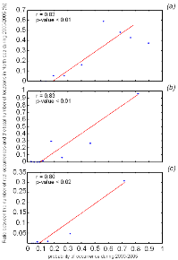
If the preferred fish prey of North Sea seabirds declines in
abundance due to a northward movement constrained by their thermal niche, it is
worthwhile speculating as to what may happen to current seabird populations.
For example, climate-driven changes in the distribution of European sardine
have been the cause of latitudinal expansion of the Balearic shearwater, from
the French Biscay coast to southern UK coasts (Yésou 2003; Wynn et
al. 2007). While it seems unlikely that European anchovy, as well as
European sardine will occur in sufficient quantity in the North Sea to become a
prevalent prey at more northern latitudes for black-legged kittiwakes and
common guillemots, some northern seabird species could expand their range
southwards to take advantage of any increase in abundance of these two fish.
Southern movements of some species previously common in the Northern North Sea
have already been observed in response to North Sea warming. This hypothesis
implicates a large plasticity for other key environmental factors such as
temperature that can become a source of physiological stress even for these
endotherm species. How quickly North Sea seabirds may acclimate to a new diet
is uncertain since most seabirds have a highly specialised diet and it is
unclear whether they have sufficient plasticity to forage on alternative prey
species (Grémillet & Boulinier 2009).
There is strong evidence that the North Sea is a tightly
coupled ecosystem controlled by the hydroclimatic environment and influenced by
trophic interactions (Kirby et al. 2009; Beaugrand & Kirby 2010a,
b). Previously, we have shown how climate-induced changes in species
composition in the benthos, plankton and among fish have altered trophic
interactions in the pelagic food web to drive the North Sea towards a new
dynamic regime favouring jellyfish in the plankton and decapods and
detritivores in the benthos over commercial fisheries. The results we report
here extend the influence of hydroclimatic change to include the putative
consequences for the small pelagic fishes of the North Sea. In other marine
ecosystems where changes in top predators due to overfishing have freed the
small planktivorous pelagic fishes from top-down control, the subsequent
increase in their abundance has comprised trophic cascades that have influenced
plankton abundance and fish recruitment (Frank et al. 2005; Daskalov
et al. 2007). The decline in abundance of planktivorous fish in the
North Sea predicted by our model may therefore reinforce further the trophic
amplification of a climate signal already witnessed in the North Sea (Kirby
& Beaugrand 2009), and also extend this to the avian fauna providing the
most comprehensive example yet of the effects of climate-induced ecosystem
change. We remind that our model and projections are highly dependent on the
intensity of warming (Beaugrand et al. In press).
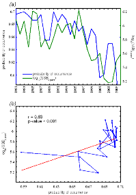
Figure IV.5 : Comparison
(a) and correlation analysis (Spearman's rank
correlation) (b) of long term changes of lesser
sandeel (two years old) spawning-stock biomasses (SSB, ICES 2010) and the
probabilities of occurrences modelled by the NPPEN in area IV for the period
1983-2006.
We used in this paper probable scenarios of SST change
(Intergovernmental Panel on Climate Change 2007b). More intense warming,
comparable to Scenario A1FI (IPCC 2007), could accelerate the biogeographic
movements and the trophic amplification in the North Sea ecosystems.
Acknowledgements
R.R.Kirby is a Royal Society Research Fellow. We thank the
Centre National de la Recherche Scientifique (CNRS) for financial support. We
thank Dr Maud Moison for helpful comments on the figures, and the IFREMER of
Boulogne-sur-Mer for helpful advice concerning IBTS surveys.
Supporting Information
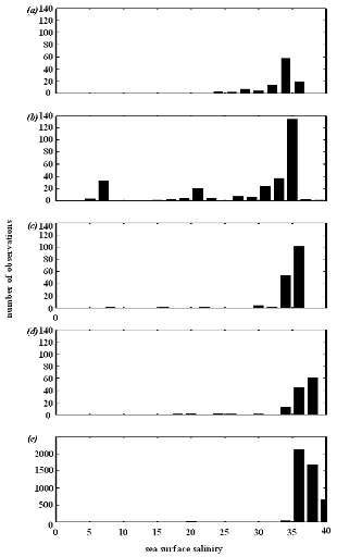
Figure IV.S1 : Salinity preferendum estimated
for (a) lesser sandeel, (b)
European sprat, (c) snake pipefish,
(d) European anchovy and (e) European sardine.
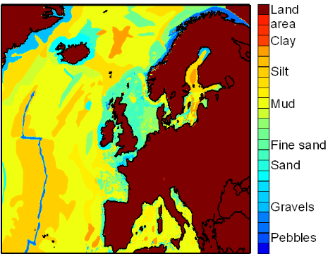
Figure IV.S2 : Spatial distribution of the
bottom-sediment type used for the estimation of lesser sandeel spatial
distribution.
Figure IV.S3 : Estimated probability of
occurrence using NPPEN for the time periods 1960-1969 (a),
2000-2008 (b), 2050-2059
(c) and 2090-2099 (d) in
the North Sea (bounding box) and adjacent seas for lesser sandeel.
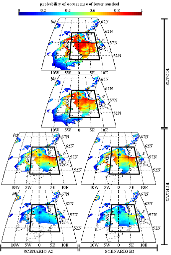
Figure IV.S4 : Estimated probability of
occurrence using NPPEN for the time periods 1960-1969 (a),
2000-2008 (b), 2050-2059 (c) and 2090-2099
(d) in the North Sea (bounding box) and adjacent seas for
European sprat
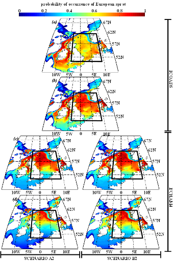
Figure IV.S5 : Estimated probability of
occurrence using NPPEN for the time periods 1960-1969 (a),
2000-2008 (b), 2050-2059 (c) and 2090-2099
(d) in the North Sea (bounding box) and adjacent seas for
snake pipefish.
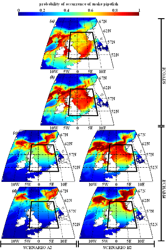
Figure IV.S6 : Estimated probability of
occurrence using NPPEN for the time periods 1960-1969 (a),
2000-2008 (b), 2050-2059 (c) and 2090-2099
(d) in the North Sea (bounding box) and adjacent seas for
European anchovy.
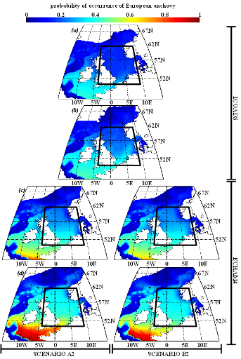
Figure IV.S7 : Estimated probability of
occurrence using NPPEN for the time periods 1960-1969 (a),
2000-2008 (b), 2050-2059 (c) and 2090-2099
(d) in the North Sea (bounding box) and adjacent seas for
European sardine.
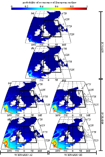
CHAPITRE V
Réchauffement climatique, Calanus
finmarchicus et la morue de l'Atlantique
1. Avant-propos
L'impact de la variabilité des facteurs
environnementaux et climatiques sur les poissons marins (O'Brien et
al., 2000) est régulièrement mis en avant pour expliquer les
variations observées des stocks de poissons. Par exemple, le recrutement
de la morue de l'Atlantique est affecté par des modifications de la NAO
(Brander & Mohn, 2004). De plus, la température est
désignée comme étant un facteur clef pour le recrutement
de la morue (Sundby, 2000 ; Björnsson et al., 2001 ;
Pörtner et al., 2001). Une étude a mis en évidence
la vulnérabilité de la morue de l'Atlantique aux changements
climatiques, quand celle-ci se trouve en bordure de sa niche thermique
(Beaugrand et al., 2010). Cette vulnérabilité climatique
est exacerbée lorsqu'elle s'applique à des populations
déjà atteintes par les effets de la surexploitation (Brander,
2005). De même, le réchauffement climatique a été
à l'origine de la réorganisation biogéographique de
certaines espèces de poissons (Parmesan & Yohe, 2003 ;
Drinkwater, 2005 ; Perry et al., 2005). En 2003, Beaugrand et
al., ont mis en évidence l'impact des variations climatiques sur la
morue de l'Atlantique via le réseau trophique et, en particulier, via la
communauté des copépodes calanoïdes, proies essentielles aux
larves et juvéniles de Gadus morhua Linnaeus, 1758
(Beaugrand et al., 2003). Plus récemment, Beaugrand & Kirby
(2010b) ont montré que les fortes probabilités de présence
de la morue coïncident avec de forte abondance de Calanus
finmarchicus à l'échelle de l'océan Atlantique
Nord.
La morue de l'Atlantique est une espèce qui a fait
l'objet d'une pêche intensive au 20e siècle
(Andrews et al., 2006) jusque dans les années 1980.
Après le pic des années 1970, le volume des captures a
commencé à chuter et ce malgré un effort de pêche
équivalent. Comprendre comment et pourquoi les stocks de morue
s'effondraient, constituait un défi de tout premier plan (Myers et
al., 1996 ; Cook et al., 1997 ; Myers et al.,
1997). Comme pour de nombreuses espèces de poisson, l'impact de la
surexploitation sur la morue de l'Atlantique est dénoncée
(Pauly et al., 2005).
Dans le contexte du changement climatique et dans le cadre de
la mise en place de plans de gestion des ressources marines, il devient
primordial d'intégrer les effets du réchauffement, pouvant
provoquer la diminution de certains stocks (Rose, 2004 ; Kirby et
al., 2009), dans les stratégies de gestion durable des pêches
(Kell et al., 2005). C'est pourquoi, de nouveaux outils basés
sur la niche écologique des espèces sont développés
pour tenter de prédire comment les poissons risquent de réagir,
en réponse au réchauffement des océans. Ces modèles
utilisent des variables écogéographiques, comme la
température, la bathymétrie, la distance à la côte
et la production primaire (Kaschner et al., 2006). La
disponibilité en proies zooplanctoniques étant une variable
critique pour des stades clefs du cycle de vie des poissons, il est essentiel
de l'utiliser comme une nouvelle dimension pour décrire la niche
écologique.
Dans ce chapitre, le modèle NPPEN est utilisé
pour modéliser la distribution spatiale potentielle passée,
présente et future de la morue en fonction (1) des trois descripteurs de
type environnemental précédemment utilisés (SST,
bathymétrie et SSS) ; et (2) d'un quatrième
descripteur : la présence du copépode calanoïde
C. finmarchicus. L'étude de l'évolution temporelle
des probabilités de présence de la morue a été
réalisée sur trois zones géographiques, pour lesquelles
une activité de pêche est, ou a été,
pratiquée : les eaux autours de Terre-Neuve, la Mer du nord (zone
CIEM IV) et les eaux islandaises (zone CIEM Va).
2. Données
utilisées
? Données biotiques
L'espèce de poisson choisie dans cette étude est
la morue de l'Atlantique (Gadus morhua). Les données de
présence de la morue proviennent, comme pour les chapitres II, III et
IV, de la base de données en ligne FishBase (Froese & Pauly, 2009),
complétée avec des données provenant du Conseil
International pour l'Exploitation de la Mer (CIEM ; ICES FishMap 2005,
2007), de la littérature et des connaissances scientifiques sur la
distribution spatiale de cette espèce. Les observations sont
datées et géo-référencées.
Le facteur biotique « proie »
utilisé dans cette étude est le copépode calanoïde
C. finmarchicus. Les données concernant la distribution
spatiale de cette espèce ont été
récupérées, à partir de cartes de
répartition géographique modélisées grâce au
NPPEN (Beaugrand et al., en préparation; Fig. V.1a).
La probabilité de présence potentielle de
C. finmarchicus a été cartographiée
annuellement de 1960 à 2100 à une résolution de 0,5°
de longitude et de latitude.
? Données abiotiques
Comme dans les chapitres précédents, les jeux de
données des trois paramètres physiques considérés
ont été compilés : la température de surface
(SST) de 1960 à 2006 (ICOADS), la bathymétrie, la salinité
de surface (SSS). Les scénarios d'évolution du climat SRES A2 et
B2 du modèle ECHAM4, de même que les scénarios SRES A1B,
B1, COMMIT et PICNTRL du modèle HadCM3, ont été inclus
pour modéliser la distribution potentielle future de la morue.
La zone géographique couverte par les trois variables
s'étend des latitudes 25°N à 85°N et des longitudes
80°W à 65°E (Fig. V.1). Les valeurs des trois variables sont
interpolées en utilisant une méthode bilinéaire avec une
résolution de 0,5° de latitude et de 0,5° de longitude, pour
créer un jeu de cartes environnementales similaires : une carte de
bathymétrie, une carte de SSS et une carte de SST par année, de
1960 à 2100.
? Zone d'études
Les zones d'études utilisées (Fig.
V.1b), pour illustrer l'évolution potentielle de la
probabilité de présence de la morue, sont les zones CIEM IV et
Va. En Atlantique Ouest, une troisième zone située autour de
Terre-Neuve est définie. Elle est limitée au sud et au nord par
les latitudes 41,5°N et 55°N et limitée à l'Ouest et
à l'Est par les longitudes ?70°O et ?41,5°O, (Fig.
V.1b).
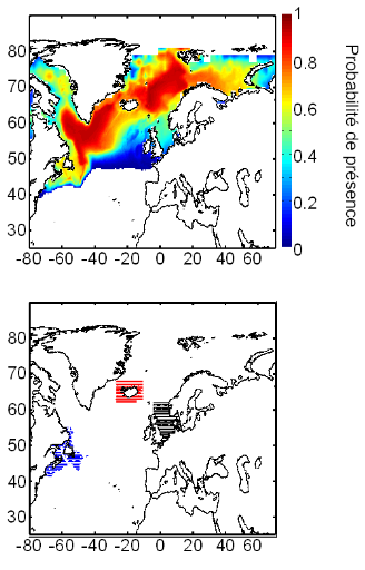
Figure V.1 : (a) distribution potentielle de
l'espèce Calanus finmarchicus durant la décennie
1960-1969 modélisée avec le modèle NPPEN à partir
de la SST, de la bathymétrie et de la SSS et (b) zones
d'étude de l'évolution annuelle des probabilités de
présence potentielle de la morue : zone
« Terre-Neuve » en bleu, zone CIEM Va (Islande) en rouge et
zone CIEM IV (mer du Nord) en noir.
3. Méthode et
Analyses effectuées
? Méthode
Nous avons utilisé la méthode NPPEN et la
méthode d'homogénéisation, lesquelles sont décrites
dans les sections précédentes.
? Analyse 1
La première analyse consistait à comparer les
résultats du modèle NPPEN utilisé avec trois descripteurs
environnementaux (SST, bathymétrie, SSS,) à ceux obtenus avec le
modèle utilisé avec trois descripteurs environnementaux et un
descripteur biotique (SST, bathymétrie, SSS, présence de
proie C. finmarchicus) (Fig. V.2). L'objet de cette analyse
était de mesurer les différences liées à
l'utilisation du paramètre biotique C. finmarchicus.
? Analyse 2
Dans cette deuxième analyse, le NPPEN a
été utilisé avec les paramètres SST,
bathymétrie, SSS, et avec ou sans le descripteur biotique
C. finmarchicus (Figs. V.3 à V.5). La probabilité
de présence moyenne de la morue de l'Atlantique a d'abord
été modélisée pour les périodes 1960-1969,
2000-2006 et 2090-2099 scénario B2 (Fig. V.3). Puis, l'évolution
annuelle moyenne des probabilités de présence de la morue a
été calculée pour chacune des trois zones de
l'étude (zone « Terre-Neuve », zone CIEM Va et zone
CIME IV), de 1960 à 2006 (Figs. V.4a et V.5a) et pour
la période de 2006 à 2100 (Figs. V.4b, c et d et
V.5b, c et d) en fonction des différents scénarios
d'évolution du climat.
? Analyse 3
La probabilité moyenne de présence de la morue
de l'Atlantique a été calculée pour les trois zones
prospectées (zone « Terre-Neuve », zone CIEM Va et
zone CIEM IV), pour chaque décennie entre 1960 et 2100 et pour chaque
scénario d'évolution du climat. Les probabilités moyennes
de présence calculées ont été distribuées en
dix classes (de 0 à 1). Les distributions en classe ont
été reportées sur les figures V.4 et V.5. Seule
l'évolution future des probabilités basées sur le
scénario B2 a été illustrée et la distribution en
classe des probabilités de présence pour la décennie
1960-1969 a été conservée dans chaque graphique à
des fins de comparaisons (histogrammes bleus).
4. Principaux
résultats obtenus
? Analyse 1
Les résultats obtenus à l'aide du modèle
NPPEN basé sur quatre paramètres (SST, bathymétrie SSS et
présence de C. finmarchicus) différent des
résultats obtenus sans la présence du paramètre biotique
« copépode » (Figs. V.2 et V.3). Par rapport au
modèle utilisé sans paramètre biotique, on note une
estimation inférieure de la probabilité de présence de la
morue de l'Atlantique en mer de Norvège, mer de Barents, mer de
Groenland, dans les eaux islandaises et aux alentours immédiats de
Terre-Neuve (Fig. V.2). Par contre, au sud de la mer Nord et en mer du
Labrador, les valeurs des probabilités de présence de la morue,
calculées par le modèle utilisant la présence de proie,
sont supérieures à celles qui sont produites sans le
paramètre biotique (Fig. V.2).
? Analyse 2
La cartographie de l'évolution des probabilités
de présence de la morue en Atlantique Nord montre un mouvement
biogéographique de cette espèce dirigé vers le Nord, entre
les périodes 1960-1969 et 2000-2006 (Fig. V.3a, b). Le
mouvement biogéographique observé est plus prononcé
côté Est de l'océan Atlantique (la mer du Nord et la mer de
Barents). À l'avenir, ce déplacement latitudinal risque de se
poursuivre, et son intensité dépend du type de scénario
d'évolution du climat choisi. L'intégration du facteur biotique
C. finmarchicus, dans la modélisation de la
présence de la morue de l'Atlantique, fournit des probabilités
généralement inférieures à celles
modélisées sans ce paramètre (Fig. V.3). L'amplitude des
changements biogéographiques est tempérée par
l'utilisation du descripteur biotique.
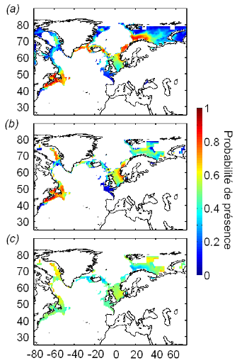
Figure V.2 : Distribution potentielle
(probabilité de présence) de la morue de l'Atlantique pour la
décennie 1960-1969 modélisée avec le NPPEN à partir
de (a) la SST, la bathymétrie et la SSS,
(b) la SST, la bathymétrie, la SSS et la
présence modélisée de C. finmarchicus, et
(c) différence des probabilités de
présence (a) - (b).
De 1960 à 2006, l'évolution annuelle des
probabilités de présence de la morue en Atlantique nord,
modélisée par le NPPEN (Figs. V.4a et V.5a),
montre trois types de situations différents. Dans la zone
« Terre-Neuve », l'évolution à long terme des
probabilités de présence est relativement stable, bien qu'avec
une variabilité interannuelle prononcée ; dans les deux cas
(présence ou non du facteur biotique dans l'analyse) les valeurs de ces
probabilités oscillent entre 0,6 et 0,7. En mer du Nord, les valeurs de
probabilités sont comprises entre 0,4 et 0,6 et sont globalement plus
faibles quand elles sont calculées sans le facteur biotique ; dans
les deux cas (présence ou non du facteur biotique dans l'analyse), une
nette tendance à la diminution dans cette zone est observée
à partir des années 1980. Dans les eaux islandaises, entre 1960
et 2006, si le facteur biotique n'est pas utilisé, les
probabilités de présence se situent entre 0,45 et 0,6, elles
semblent avoir déclinées très légèrement
jusque dans les années 1990, années à partir desquelles
elles ont entamé une hausse ; si le facteur biotique est pris en
compte, les probabilités de présence calculées sont
inférieures à 0,35 et aucune tendance à l'augmentation ou
la diminution n'est observée de façon nette.
De 2006 à 2100, l'évolution annuelle des
probabilités potentielles de présence de la morue de l'Atlantique
(Figs. V.4 et V.5), montre qu'en zone
« Terre-Neuve » (Figs. V.4b et V.5b),
seuls les scénarios SRES A2 et B2 (lignes bleues) provoquent une chute
importante et rapide des probabilités de présence de la morue de
l'Atlantique. Avec les scénarios A1B et B1, les probabilités de
présence se maintiennent à un niveau stable jusqu'en 2070 ;
avec les autres scénarios, COMMIT et PICNTRL, les probabilités de
présence n'évoluent pas. L'utilisation ou non du paramètre
biotique n'a pas d'influence sensible sur l'évolution des
probabilités en zone « Terre-Neuve ». En Mer du Nord
(Figs. V.4c et V.5c), seuls les scénarios COMMIT et
PICNTRL (lignes verte et turquoise) prévoient le maintient d'une
présence équivalente à celle actuelle. Tous les autres
scénarios prédisent une chute progressive et irréversible
de la présence de la morue; l'utilisation ou non du paramètre
biotique n'a pas d'influence sensible sur l'évolution des
probabilités. Enfin, en Islande (Figs. V.4d et
V.5d), l'analyse pratiquée, sans le facteur biotique, montre
une stabilisation des probabilités à un niveau plus faible
qu'avant 2006 quelque soit le scénario utilisé. Une hausse
très faible des valeurs des probabilités de présence
annuelles est attendue, dans le cas où le facteur
« présence de proie » est considéré
(Fig. V.5d).
Figure V.3 : Distribution potentielle
(probabilités de présence) de la morue de l'Atlantique pour les
périodes temporelles 1960-1969 (a), 2000-2006
(b) et 2090-2099 scénario B2(c),
modélisée avec le NPPEN. Les paramètres pris en compte
sont : la SST, la bathymétrie, la SSS (colonne de gauche et droite)
et la présence modélisée par le NPPEN de C.
finmarchicus (colonne de droite).
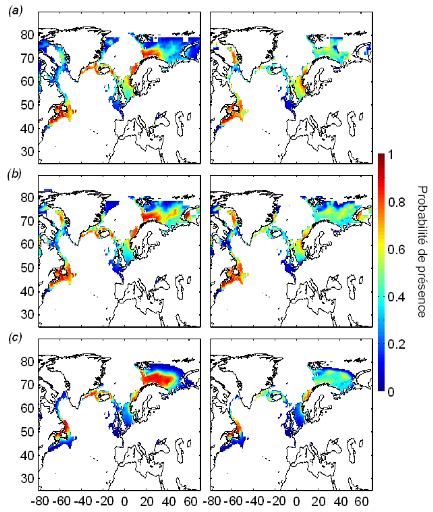
? Analyse 3
Les trois régions marines constituent des habitats aux
potentiels d'accueil de la morue différents et fluctuants dans le temps
(Figs. V.4e, f et g et V.5e, f et g).
L'étude de l'évolution des probabilités
de présence, entre les périodes 1960-1969 et 1980-1989, montre
peu de changements et ce quelque soit la zone considérée. Entre
les périodes 1960-1969 et 2000-2006, des changements sont observables en
mer du Nord uniquement, représentés par un affaiblissement dans
leur ensemble des probabilités de présence de la morue (Figs.
V.4f et V.5f). Après 2050, seule la zone CIEM Va
islandaise conserve une distribution de probabilités similaire à
celle des années 1960-1969. En mer du Nord, le glissement de la
majorité des probabilités vers des valeurs plus faibles
s'accentue. Du côté de Terre-Neuve, le même
phénomène est prédit à partir de la période
2050-2059.
La comparaison de la décennie 1960-1969 entre les
figures V.4 et V.5 montre que, de façon général,
l'utilisation du paramètre biotique ne modifie pas la distribution des
probabilités de présence en zone
« Terre-Neuve ». En mer du Nord, l'utilisation du
paramètre biotique estime les probabilités supérieures
(entre 0,6 et 0,8) à celles produites sans ce paramètre (entre
0,4 et 0,6). Dans les eaux islandaises, l'utilisation du paramètre
biotique ne permet pas aux probabilités de présence de
dépasser la valeur 0,7. Sans le paramètre biotique, le
modèle évalue que les probabilités de présence de
la morue peuvent atteindre la valeur de 0,9.
L'évolution des probabilités de présence
de la morue de l'Atlantique, décennie par décennie,
diffère sensiblement quand est pris en compte le facteur biotique proie
dans le modèle. Dans la zone « Terre-Neuve »,
l'utilisation du facteur biotique concentre un peu plus les probabilités
de présence vers des valeurs très faibles proche de 0,1. En mer
du Nord, le glissement vers des valeurs plus faibles de la distribution des
probabilités s'opère entre les périodes 1960-1969 et
2000-2006, mais il est moins intense quand est inclut le facteur biotique proie
dans la modélisation. Autour de l'Islande, l'évolution des
probabilités de présence ne semble pas être affectée
par l'utilisation ou non du paramètre biotique proie.
Figure V.4 : Évolutions annuelles
de la probabilité de présence de la morue calculée, sans
C. finmarchicus, à Terre-Neuve (en bleu), en mer du Nord (en
noire) et en Islande (en rouge) modélisées, par le NPPEN de 1960
à 2006 (a) et en fonction des scénarios
d'évolution du GIEC Terre-Neuve (b) en mer du Nord
(c) et en Islande (d). Comparaison des
distributions des probabilités de présence de la morue, entre les
périodes 1960-1969/1980-1989, 1960-1969/2000-2006, 1960-1969/2050-2059
et 1960-1969/2090-2099, à Terre-Neuve (e), en mer du
Nord (f) et en Islande (g).
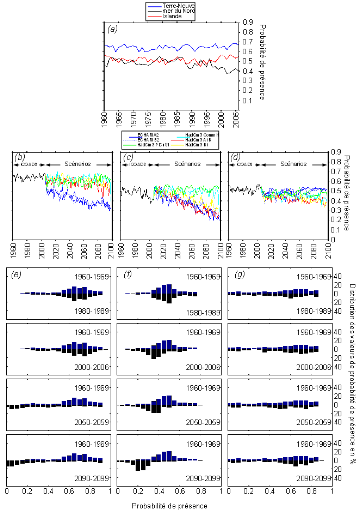
5. Discussion
L'objectif de ce chapitre était d'appliquer le
modèle NPPEN pour modéliser la distribution spatiale de la morue
de l'Atlantique, en utilisant une dimension supplémentaire pour en
définir la niche écologique: la présence de sa proie
C. finmarchicus. Cette étude permet d'effectuer une
comparaison des performances du modèle, utilisé avec ou sans ce
paramètre biotique essentiel pour la survie des larves de morue de
l'Atlantique.
Kirby & Beaugrand (2009) ont mis en évidence
l'amplification de l'impact du réchauffement climatique le long de la
chaine trophique en mer du Nord, depuis les organismes planctoniques jusqu'aux
poissons. Les résultats obtenus dans ce chapitre montrent des
probabilités de présence de la morue différentes quand le
paramètre biotique proie est utilisé. La présence de
C. finmarchicus comme descripteur dans le modèle augmente
les valeurs de probabilité de présence de la morue au sud de la
mer du Nord, en mer de Barents et au nord de Terre-Neuve, mais baisse les
valeurs de probabilités le long des côtes norvégiennes et
au sud du Québec (Figs. V.2 et V.3). Le phénomène de
déplacement biogéographique vers le nord, qui affecte la morue de
l'Atlantique, semble atténué ou comme ralenti (Fig. V.3 à
V.5) quand est utilisé le facteur proie, pour cartographier et estimer
la présence de la morue au cours des décennies 2050-2059 et
2090-2099.
L'examen des cartes de distribution de l'espèce
C. finmarchicus modélisées par le modèle
NPPEN (décennie 1960-1969 Fig. V.1), révèle une estimation
de la présence de ce copépode en mer du Nord inférieure
à celle réellement observée (CPR Team, 2004).
Figure V.5 : Évolutions annuelles
de la probabilité de présence de la morue, calculée avec
C. finmarchicus, à Terre-Neuve (bleu), en mer du Nord (noir) et
en Islande (rouge), modélisées par le NPPEN de 1960 à 2006
(a), et en fonction des scénarios d'évolutions
du GIEC à Terre-Neuve (b), en mer du Nord
(c) et en Islande (d). Comparaison des
distributions des probabilités de présence de la morue, entre les
périodes 1960-1969/1980-1989, 1960-1969/2000-2006, 1960-1969/2050-2059
et 1960-1969/2090-2099 à Terre-Neuve (e), en mer du
Nord (f) et en Islande (g).
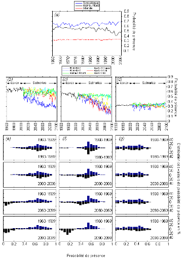
Un des objectifs de ce chapitre était d'utiliser le
modèle NPPEN pour comprendre les évolutions différentes
des stocks de morues dans des régions distinctes de l'Atlantique Nord.
Beaugrand & Kirby (2010a) ont montré que des stocks de morues en
Atlantique Nord-Est, aux répartitions géographiques bien
distinctes (un en mer du Nord et un en Islande) réagissaient
différemment au forçage climatique. La différence dans
leur répartition géographique correspond une différence
dans leur localisation au sein de la niche écologique. Des populations
présentes dans les régions comme la mer du Nord, se situant en
limite inférieure de la niche écologique
(préférendum thermique centré sur des températures
entre 9°C et 10°C), seront plus sensibles à de petites
modifications de la température de leur environnement. En Islande, les
eaux marines plus froides sont en adéquation avec le centre de la niche
thermique de la morue, le réchauffement climatique est moins susceptible
d'y influencer les populations. Outre-Atlantique, les eaux de Terre-Neuve
disposent de conditions climatiques et environnementales restées
à la fois stables et favorables à la présence de
l'espèce. D'après les résultats obtenus dans ce chapitre,
la disparition et la non-reconstruction des stocks au Canada, malgré la
mise en place de moratoires de pêche pour limiter les conséquences
de la surexploitation (Pauly, 1998 ; Pauly et al., 1998 ;
Christensen et al., 2003 ; Worm et al., 2005), ne sont
pas dues à un changement de l'environnement occupé par la morue
l'Atlantique mais bien à l'exploitation intensive qu'a subit cette
espèce. En mer du Nord, la situation est différente, petit
à petit, cette zone devient défavorable à la
présence de la morue. Ainsi, la chute constatée dans les
débarquements (Brander et al., 2006) ne peut être
imputée uniquement à l'effet de la surpêche dans cette
zone.
DISCUSSION
CONCLUSIONS
PERSPECTIVES
1. Discussion
1.1. Le modèle
NPPEN
La recherche réalisée dans le cadre de cette
thèse s'est appuyée sur le concept de la niche écologique,
sensu Hutchinson, et d'un modèle d'habitat. Cette
démarche a permis de (1) cartographier la distribution spatiale moyenne
des poissons et (2) de proposer des scénarios d'évolution
géographique des ressources marines et spécialement des poissons
marins à fort intérêt commercial ou écologique. Ce
travail s'inscrit dans le contexte très particulier du changement
climatique, où la distribution des espèces risque de subir de
forts déplacements latitudinaux (Parmesan & Yohe, 2003 ;
Deutsch et al., 2008). Pour pouvoir évaluer l'impact du
réchauffement climatique sur la répartition spatiale des poissons
marins, il convient de disposer d'informations fiables sur leur distribution
spatiale actuelle. Or, il s'avère que ces informations restent encore
parcellaires, le plus souvent représentées sous la forme d'un
trait côtier (Louisy, 2002) ou d'un ombrage (FAO) sur une carte,
codées de façon binaire (présence certaine, absence).
Nous avons donc créé un nouveau modèle
d'habitat basé sur la distance généralisée de
Mahalanobis et proposons, pour la première fois, un test
non-paramétrique pour évaluer sa significativité. Le
modèle d'habitat NPPEN cartographie la distribution spatiale d'une
espèce en fonction de l'adéquation entre les contraintes de sa
niche écologique et les ressources offertes par l'habitat disponible. Ce
modèle a le très gros avantage de ne requérir que des
données de présence, ce qui le rend fort utile à
macro-échelle pour étudier la biogéographie des
espèces marines, pour lesquelles les données de présence
sont seules disponibles (Brotons et al., 2004 ; Guinotte et
al., 2006). Le nouveau modèle NPPEN est donc plus adapté
pour répondre aux objectifs de la thèse que les modèles
fonctionnant obligatoirement à partir de la présence et l'absence
ou basé sur l'abondance, tels les modèles additifs
généralisés (GAM ; Hastie & Tibshirani, 1990),
les modèles linéaires généralisés
(GLM ; McCullagh & Nelder, 1983), les méthodes neuronales
(ANN ; Lek et al., 1996 ; Mastrorillo et al., 1997)
ou les arbres de classification (CART, Thuiller et al.,2003).
L'autre avantage, conféré par l'utilisation de
données d'observation pour reconstruire la niche écologique, est
de ne pas en définir les contours de façon arbitraire et de ne
pas avoir besoin d'utiliser de seuils ou de règles de décision
pour en déterminer les limites. En ce sens, le NPPEN constitue une
alternative aux modèles déjà existants, utilisés
pour certains dans le milieu marin (Rose, 2005 ; Kaschner et al.,
2006 ; Cheung et al., 2008a, b). Ces outils décrivent la
niche écologique sous différentes formes, conditionnant ainsi
leurs prédictions. Les modèles BIOCLIM, HABITAT et le
modèle AquaMaps (Kaschner et al., 2007), sont basés sur
une niche écologique aux formes imposées, décrivant
respectivement : un volume rectiligne, une enveloppe convexe et un
trapèze (Carpenter et al., 1993 ; Kaschner et
al., 2006). Cette vision simplifiée de la niche comporte le risque
d'exclure, de façon non justifiée, des points
géographiques de l'aire de répartition des organismes (Carpenter
et al., 1993). Ainsi, il est primordial, avec ce genre de
modèle, de définir le plus justement possible les contours de la
niche, et donc d'avoir une bonne connaissance des exigences environnementales
de l'espèce étudiée. En 1993, Carpenter et al.
(1993) pour résoudre ces problèmes, présentèrent le
modèle DOMAIN qui utilise la métrique de similarité point
par point de Gower (Legendre & Legendre, 1998). Néanmoins, un seuil
de significativité de cette métrique doit être
établi. De la même façon, le modèle de l'entropie
maximale (MAXENT ; Philips et al., 2006) a besoin qu'un seuil
précis et exact soit défini pour pouvoir fournir des
résultats robustes.
La quantité et la qualité des données de
présences sont des paramètres déterminant pour tous les
types de modèles d'habitat (Stockwell & Peterson, 2003). La
pré-procédure d'homogénéisation du modèle
NPPEN permet d'éviter les problèmes liés à
l'absence de plan d'échantillonnage. Les données sont fortement
hétérogènes. Si souvent
l'hétérogénéité est réelle (Fig.
III.2 et Figs. Annexes III.S3-S9), elle peut parfois subvenir à cause du
contexte socio-économique (concentration de la pêche dans certains
secteurs déterminée par le contexte juridique ou
économique). Les espèces étudiées ne
présentent pas toutes les mêmes intérêts commerciaux
et scientifiques. De plus, des espèces rares ou à la niche
écologique très étroite, ou encore des espèces
migratrices à la niche écologique multimodale, peuvent ne pas
être observées en quantité suffisante pour pouvoir
valablement estimer les contours de la niche. La procédure
d'homogénéisation qui a été mise en place a permis
d'améliorer significativement la modélisation par le
modèle NPPEN (Figs. II.6 et III.3). L'exemple de la modélisation
de la distribution spatiale d'organismes tels que le sprat européen ou
Calanus finmarchicus illustre le comportement différent du
NPPEN, en fonction de la représentativité des données de
présence. Bien qu'en nombre réduits, les données de
présence du sprat européen (Chapitre III) sont réparties
sur la totalité de la niche et permettent donc une modélisation
de la distribution spatiale satisfaisante. Par contre, les données de
présence de C. (Chapitre V), bien qu'en très grand
nombre, étaient concentrées que sur un sous-ensemble de la niche.
Il a été donc nécessaire de compléter la niche
empiriquement.
Le caractère non-paramétrique du test de
permutations du modèle NPPEN permet de s'affranchir du besoin de la
normalité des variables utilisées, avantage très
intéressant en écologie, où cette condition est rarement
remplie (exemple : la bathymétrie). La normalité des
données limite l'application de modèles tels que l'analyse
factorielle de la niche écologique (ENFA ; Hirzel, 2001 ;
Hirzel et al., 2002) pour laquelle des transformations de
normalisation sont indispensables au préalable. Enfin, le faible nombre
de variables environnementales utilisées pour décrire la niche
écologique des espèces (température de surface,
bathymétrie, salinité et nature du fond, Figs II.1, III.2 et
IV.S1-S2) peut être considéré comme un désavantage
ou une limitation, de prime abord. Toutefois, à macro-échelle, un
soin particulier dans le choix des descripteurs par une connaissance rigoureuse
des facteurs qui influent le plus sur la distribution des organismes, par
exemple en effectuant une analyse en composantes principales (ACP), permet de
considérer comme bénéfique ce faible nombre de
descripteurs utilisés, faisant du modèle NPPEN un outil simple
aux paramètres d'utilisation (« inputs ») facilement
définissables.
Le modèle NPPEN est basé sur la distance
généralisée de Mahalanobis (Mahalanobis, 1936). Cette
distance prend en compte les différences d'échelles entre les
descripteurs environnementaux, contrairement à la distance Euclidienne
ou à la distance de Gower utilisée dans le modèle DOMAIN
(Legendre & Legendre, 1998). Elle considère aussi la
corrélation entre descripteurs, ce que ne permettent ni la distance
Euclidienne et a fortiori la distance de corde (Fig. II.4).
Comme tous les modèles d'habitat, le modèle
NPPEN est probablement sensible à l'autocorrélation spatiale des
données abiotiques. (Diniz-Filho et al., 2003 ; Segurado
et al., 2006 ; Dormann, 2007). Cependant,
l'autocorrélation spatiale semble toucher plus fortement les techniques
de régressions telles que le GAM ou le GLM (Dormann, 2007) et ses
possibles effets sur le NPPEN sont limités par la procédure
d'homogénéisation utilisée dans la préparation des
données. Nous avons aussi noté un effet de bord
géographique avec le modèle NPPEN. Les probabilités de
présence calculées en limite géographique (interface
continent et mer) sont à interpréter avec plus de
précautions. En effet, la probabilité peut chuter fortement
près de telles interfaces sans raison écologique (Fig. II.6). Cet
effet peut être limité empiriquement (voir Reygondeau &
Beaugrand 2010).
A la vue de ces différents avantages, la distance de
Mahalanobis est une métrique de plus en plus utilisée dans les
modèles d'habitat. Néanmoins, l'approche NPPEN est
également novatrice dans la façon dont est utilisée cette
distance. Le NPPEN teste la distance de Mahalanobis par un test non
paramétrique de permutations qui provient d'une simplification du test
proposé par (Mielke et al., 1981, Beaugrand &
Healouët, 2008). Ce test a l'avantage de fournir des probabilités
de présence plutôt que de se contenter de classer les distances
mesurées par déciles (Nogués-Bravo et al., 2008)
et, de s'affranchir de la multi-normalité des variables contrairement au
D² testé par un ÷² (Ibañez, 1981) ou
à la procédure de décomposition factorielle de la distance
de Mahalanobis (MADIFA ; Calenge et al., 2008).
1.2. Impacts du réchauffement climatique sur la
distribution spatiale des poissons marins
Les dernières estimations scientifiques font
état d'un réchauffement global du système
planétaire d'environ 0,8°C depuis le début du 20e
siècle. Les observations indiquent que 84% du réchauffement du
système planétaire a eu lieu dans les océans
(Intergovernmental Panel on Climate Change, 2007b). Une des premières
conséquences attendues du changement climatique sur les organismes
vivants est le déplacement latitudinal des espèces vers les
pôles (Parmesan & Yohe, 2003). Ce mouvement biogéographique a
déjà été observé à la fois dans le
milieu terrestre et dans le milieu marin (Thomas & Lennon, 1999; Beaugrand
et al., 2002a; Parmesan & Yohe, 2003; Perry et al.,
2005). Les scientifiques ont pu estimer et chiffrer la distance parcourue par
les espèces au cours de ces mouvements biogéographiques. Une
méta-analyse réalisée sur plus de 1700 espèces ou
groupes taxonomiques, a montré une migration moyenne de l'ordre de 610
m.an-1 pour 279 de ces espèces au cours du siècle
dernier (Parmesan & Yohe, 2003). Thomas & Lennon (1999) ont
détecté, chez 59 espèces d'oiseaux terrestres au
Royaume-Uni, un déplacement latitudinal de 945 m.an-1 entre
la fin des années 1970 et 1990. Au 20e siècle, plus de
la moitié des espèces de papillons européens ont
effectué un déplacement biogéographique à la
vitesse moyenne de 5 km.an-1 (Parmesan et al., 1999).
Les changements biogéographiques, mis en
évidence dans le milieu marin, sont plus prononcés notamment en
raison de l'absence de barrière physique entre les différentes
régions océaniques. En 2009, Beaugrand et al. (2009) ont
calculé qu'un groupe d'espèces pseudo-océaniques
caractéristiques des eaux tempérées-chaudes s'était
déplacé de 1000 km en moyenne vers le Nord, en 48 ans et à
raison de plus de 23 km en moyenne pas an. Ces changements ont
été clairement détectés le long des côtes
européennes. Un assemblage d'espèces de copépodes
calanoïdes, jadis présent uniquement dans le golfe de Gascogne, est
maintenant identifié jusqu'à l'ouest des côtes
norvégiennes, représentant un mouvement biogéographique de
près de 1000 km en une vingtaine d'années (Beaugrand et al.,
2002a). Certains isothermes ont migré de 19 km par an en moyenne
sur la même période. En parallèle, de nombreuses
études ont rapporté l'apparition d'espèces de poissons
tropicaux, nouvelles dans le golfe de Gascogne, et leur migration progressive
le long du talus continental européen jusque dans les eaux britanniques
et la mer du Nord (Quéro et al., 1998 ; Brander et
al., 2003, Stebbing et al., 2002). Une étude
récente a analysé les changements à long-terme de la
répartition spatiale de 90 espèces de poissons en mer du Nord
(Perry et al., 2005). Durant la période étudiée
(1977 à 2001), la mer du Nord s'est réchauffée d'à
peine 1,05°C en moyenne. Pourtant sur les espèces de poissons ayant
leur limite nord ou sud de répartition dans la mer du Nord (36
espèces), 15 ont migré en réponse au réchauffement
des eaux.
Le modèle NPPEN produit des cartes de distributions
spatiales actuelles des espèces, comparables et complémentaires
à celles obtenues à partir d'autres modèles (RES, FAO,
Cheung et al., 2008, 2009), ou à partir des connaissances des
scientifiques et professionnels de la pêche (ICES-FishMap ;
http://www.ices.dk/marineworld/ices-fishmap.asp ; Louisy, 2002). Durant
cette thèse, le NPPEN a également été
utilisé pour modéliser la distribution spatiale passée et
future des poissons et notamment celle des espèces
commercialisées. L'objectif était d'estimer si le NPPEN pouvait
retracer et quantifier, en termes de surface d'habitat, les changements
biogéographiques observés chez les poissons marins depuis 1960 et
d'évaluer ces changements dans le futur.
Les cartes de distribution obtenues montrent, effectivement,
une réorganisation de la distribution spatiale de toutes les
espèces étudiées entre la décennie 1960-1969 et la
période 2000-2005 (Figs. III.V et S11 à S19). Basé sur
l'ensemble de l'océan Atlantique Nord, le calcul des pertes et gains
d'habitats géographiques montre des bilans contrastés. Les
espèces comme le sprat, l'anchois, et la sardine européens, aux
préférendums thermiques plus chauds, sont les espèces qui
ont gagné le plus d'habitat potentiel, entre 200 000 et
300 000 km², suivies par l'églefin et la sole commune dans une
moindre mesure (moins de 100 000 km²). En revanche le turbot n'a pas
gagné de nouvelles zones d'habitat et les deux espèces de lieu,
aux préférendums thermiques plus froids, en ont perdu.
L'intensité du réchauffement climatique
(scénarios A2 ou B2) va définir la valeur des bilans
biogéographiques des espèces à affinités
tempérées-chaudes (A2 ou B2). Par exemple, la sole commune et le
chinchard de l'Atlantique verront leurs distributions se réduire dans le
cas d'un scénario A2, le plus pessimiste, alors qu'une évolution
des températures de type scénario B2 leur permettront de
coloniser de grandes surfaces. Par contre, les espèces dites
tempérées ou subarctiques connaîtront, quelque soit le
scénario d'évolution, une réduction de leur surface
d'habitat. La vitesse de cette perte sera sensible au scénario
d'évolution des températures. Ces chiffres font juste le bilan
des gains et des pertes, l'étude plus précise des cartes (Fig.
III.) situe mieux les endroits où auront lieu ces modifications.
Les poissons marins seront très probablement dans
l'incapacité de s'acclimater à l'échelle d'un
demi-siècle à de nouvelles contraintes environnementales
(Helaouët & Beaugrand, 2009 ; Beaugrand & Kirby, 2010a). Les
modifications biogéographiques des poissons modélisées en
Atlantique Nord (Figs. II.7 et III.4 et Annexes III.S10-III.S19) constituent
leurs réponses face aux modifications de leurs habitats. Les valeurs des
paramètres environnementaux de l'habitat disponible ne seront plus en
adéquation avec les domaines de tolérance des espèces
vis-à-vis de ces paramètres, en d'autres termes, l'habitat ne
remplira plus les conditions de la niche écologique des espèces.
Un tel mécanisme n'est pas sans conséquences sur la
viabilité des populations, amenées à effectuer ces
déplacements biogéographiques. Celles-ci ne sont pas
assurées de trouver une autre aire de répartition valable,
permettant leur pérennisation. Il en résulte un
phénomène de contractions de l'aire de répartition pouvant
conduire à la disparition d'un organisme. Par exemple, au milieu du
Pléistocène (?300 000 ans avant J.C.), un
réchauffement climatique naturel a provoqué une réduction
et une fragmentation de l'habitat du mammouth laineux (Mammuthus
primigenius, B ; Nogués-Bravo et al., 2008). De
plus, toutes les espèces n'ont pas les mêmes capacités de
déplacements, nécessaires pour rester dans un milieu en
adéquation avec leur niche (Pearson, 2006).
La vitesse des changements de répartition des
différentes espèces va être réglée par leur
capacité « migratrice » mais surtout par la largeur
de leur niche. Une espèce au préférendum thermique plus
spécialisé sera amenée à répondre plus vite
au réchauffement des eaux. L'incertitude, sur la vitesse et l'ampleur
des changements modélisés par le NPPEN, est illustrée par
l'utilisation des différentes familles de scénarios
d'évolution du climat, du plus modéré au plus fort (Fig.
II.10) (Beaugrand et al., In Press). De plus, au sein d'une
espèce, l'impact du climat sur les poissons, n'est pas le même
selon que la population étudiée se trouve géographiquement
en limite ou au centre de sa niche. Les populations de morues de l'Atlantique
situées en mer du Nord, sont en limite inférieure de leur niche
écologique. Elles sont donc plus sensibles au réchauffement des
eaux que celles situées géographiquement dans les eaux
islandaises où le régime thermique correspond au centre du
préférendum thermique de l'espèce (Beaugrand & Kirby,
2010a, b).
Si les scientifiques des pêches ont
développé un grand nombre d'outils pour simuler et tenter de
prédire la dynamique des stocks de poissons exploités (Hilborn
& Walters, 1992 ; Daskalov, 1999 ; Cardinale & Svedäng,
2004 ; Miller, 2007), les modèles prédisant les effets du
climat sur les mêmes ressources commencent seulement à être
utilisés (Kaschner et al., 2007, Cheung et al.,
2008a). Pourtant, l'un des enjeux des plans de gestion durable des stocks de
poissons est de pouvoir comprendre et anticiper les effets conjoints, et
interactifs, de la pêche et du réchauffement climatique
(Jurado-Molina & Livingston, 2002; Rose, 2004 ; Lehodey et
al., 2006 ; Mieszkowska et al., 2007 ; Rouyer et
al., 2008). Ces effets peuvent être additifs ou multiplicatifs, la
surexploitation augmentant la sensibilité des stocks de poissons et de
l'écosystème marin à la variabilité climatique
(Perry et al., 2010 ; Planque et al., 2010). Agissant en
synergie, l'impact conjoint de l'exploitation et du réchauffement
climatique peut précipiter l'effondrement de stocks de poissons, comme,
par exemple, celui de la morue de l'Atlantique en mer du Nord (Ottersen et
al., 2006 ; Beaugrand et al., 2008 ; Kirby et
al., 2009).
1.3. Propagation du réchauffement climatique le long du
réseau trophique
L'hypothèse d'un effet
« junk-food » (Wanless et al., 2005 ;
Österblom et al., 2008) est un concept
régulièrement utilisé pour expliquer les déclins
observés de populations d'organismes du milieu marin, lors de la
survenue de profonds changements dans la qualité de leurs ressources
alimentaires (Harris & Wanless, 1997 ; Romano et al.,
2006 ; Österblom et al., 2008). En cas
d'indisponibilité de proies de bonne qualité, les espèces
sont dans l'obligation soit, d'augmenter leurs efforts et leurs dépenses
d'énergie à la recherche de nourriture, soit d'utiliser une ou
plusieurs ressources disponibles, de qualité pas forcément
équivalente (Whitfield, 2008). La restructuration de
l'écosystème peut être causée par des changements
biogéographiques et phénologiques, induits par le climat
(Weijerman et al., 2005 ; Alheit, 2007). En mer du Nord, l'impact
du changement de régime des années 1980 s'est
répercuté et amplifié le long du réseau trophique,
des producteurs primaires, en passant par les consommateurs supérieurs,
impactant même les détritivores (Reid, 2005 ; Kirby &
Beaugrand, 2009). Ces changements ont contribué par exemple à la
diminution du taux de survie des larves de morue de l'Atlantique, expliquant en
partie l'importante chute de la biomasse des reproducteurs observée en
mer du Nord (Beaugrand et al., 2003). Dans le Pacifique Nord, entre
l'Alaska et la Russie, les otaries de Steller (Eumetopias jubatus
Schreber, 1776) ont du faire face à un changement dans la
disponibilité et la diversité de leurs proies, modulé par
la variabilité climatique (Francis et al., 1998 ;
Lehodey et al., 2006). Elles ont pu changer leur régime
alimentaire composé habituellement de harengs et de lançons pour
un régime basé sur le lieu et la goberge, beaucoup plus faibles
en qualité énergétique, mais en abondance bien
supérieure (Rosen & Trites, 2000). La plasticité du
régime et le comportement alimentaire des espèces vont
conditionner leur résilience à cet effet
« junk-food » (Grémillet et al.,
2008 ; Österblom et al., 2008).
Durant ces 40 dernières années, les oiseaux
marins de la mer du Nord ont connu des chutes dans leur succès de
reproduction. Cette chute est en partie reliée à un changement de
dominance des proies (Frederiksen et al., 2005 ; Wanless et
al., .2005). Le lançon nordique et le sprat européen,
espèces consommées préférentiellement par les
oiseaux, tels que le guillemot de Troïl (Uria aalge, P)
ou la mouette tridactyle (Rissa tridactyla, L) en mer du Nord, ont
connu depuis 2004 d'importantes variations de leur abondance ou de leur
qualité énergétique individuelle (Wanless et al.,
2005, 2007). En parallèle, l'entélure, espèce à la
valeur énergétique très faible (Harris et al.,
2007, 2008), a vu sa population augmenter (Kirby et al., 2006 ;
Fleischer et al., 2007 ; van Damme & Couperus, 2008) et est,
donc, de plus en plus observé dans les captures des oiseaux. Les
mouettes tridactyles, appartenant à de nombreuses colonies d'Angleterre
et d'Écosse, qui ont nourri leurs poussins avec l'entélure ont
connu un succès reproducteur très faible en 2005 et 2006 (Mavor
et al., 2006, 2008 ; Harris et al., 2007, 2008). De
nombreux poussins nourris avec de l'entélure ont été
retrouvés morts au nid, soit étouffés par une proie qu'ils
ont été incapables de gober dans son intégralité,
soit de malnutrition n'ayant pas d'autres proies proposées par les
adultes.
Au cours de cette thèse, le nouveau modèle NPPEN
a été utilisé pour évaluer si des changements
biogéographiques des espèces communément consommées
par les oiseaux marins, pouvaient expliquer le patron de disponibilité
des proies observé en mer du Nord. Les résultats montrent
qu'effectivement, la mer du Nord en se réchauffant ne peut plus
répondre aux exigences de la niche écologique du lançon
nordique, centrée autour de 8 et 12°C (Figs. IV.2a,b et
IV.3a). Il en résulte une chute de l'abondance du lançon
nordique. En parallèle, est observée une augmentation de la
présence du sprat européen et de l'entélure, aux niches
thermiques centrées entre 8 et 15°C (Figs. IV.1, IV.2a,b et IV.3a).
Ces changements ont pu être retrouvés par modélisation
grâce au NPPEN. Le modèle montre une chute de la
probabilité de présence moyenne du lançon nordique en mer
du Nord, de 0,7 à 0,5 entre 1995 et 2006. Durant la même
période, les probabilités de présence moyennes de
l'entélure et du sprat européen sont passées de 0,5
à 0,8 (Fig. IV.2).
Si le réchauffement de la mer du Nord se poursuit, la
température va progressivement sortir des limites du
préférendum thermique du lançon nordique (13°C).
L'abondance de ce poisson en mer du Nord, selon les prédictions
effectuées par le modèle NPPEN, risque de poursuivre sa chute
(Fig. IV.3b), conduisant à une disparition du lançon nordique des
eaux de la mer du Nord (Fig. IV.2a). L'alternative « sprat
européen » pourra rester valable jusqu'au milieu du
siècle, à condition que les individus retrouvent une valeur
énergétique suffisante (Fig. IV.3b). L'arrivée
d'espèces comme l'anchois et la sardine européens, par la
façade Atlantique, pourrait constituer une ressource de substitution, si
la plasticité du régime alimentaire des oiseaux le permet
(Grémillet et al., 2008). Dans le Pacifique, les Guillemots de
Troïl ont trouvé une alternative à la raréfaction,
induite par l'augmentation des températures durant
l'évènement El-Niño de 1992-1993, de leurs proies
habituelles représentées par plusieurs espèces du genre
Sebastes (Sebastes spp), en se nourrissant d'anchois californiens (Oedekoven
et al., 2001). En revanche, la possibilité qu'auront la sardine
et l'anchois européens à s'établir en mer du Nord est
très faible (Fig. IV.2 et IV.3). En effet, leurs
préférendums thermiques sont centrés autour de 18 et
20°C (Fig. IV.1c et d), ces températures ne seront pas atteintes en
mer du Nord durant ce siècle. L'éventualité d'un
déplacement des populations d'oiseaux vers le nord, pour suivre la
ressource, et donc de rester dans un environnement favorable, fait l'objet de
recherches (Peterson et al., 2002 ; Huntley et al.,
2008 ; Gregory et al., 2009). Cette possibilité semble
être fonction de la vitesse de réaction des oiseaux marins aux
changements induits par le climat sur leurs habitats habituels (Devictor et
al., 2008).
L'application du modèle d'habitat NPPEN sur les proies
des oiseaux marins permet de visualiser les changements possibles dans la
biogéographie d'espèces de niveaux trophiques différents
et les désynchronisations de ces changements entre proies et
prédateurs. Nos projections dépendent de l'intensité du
réchauffement. Un réchauffement plus fort du type A1FI ("Fossil
Intensive" ; IPCC, 2007b) pourra conduire à des altérations
plus fortes et surprenantes de la trophodynamique de l'écosystème
de la mer du Nord. À l'avenir les modèles d'habitat pourront
permettre de comprendre et prévoir ces changements ainsi que leurs
conséquences sur l'écosystème marin. Le cas de la morue de
l'Atlantique, espèce à fort intérêt commercial,
évoqué auparavant, est un exemple qui montre l'importance
d'outils capables de prédire les conséquences des changements
biogéographiques qui ont lieu au sein de l'écosystème
marin pour les professionnels de la pêche.
2. Épilogue
2.1. Conclusions
Cette thèse s'est déroulée dans le cadre
des Conventions Industrielles de Formation par la Recherche (CIFRE), entre
scientifiques et professionnels du secteur de la pêche : les
Collectivités Maritimes Étaploises (CME). L'objectif de ce projet
était d'évaluer l'impact du changement climatique sur les
ressources halieutiques dans l'océan Atlantique Nord-Est et d'en
prévoir l'évolution si le réchauffement global se
poursuit. L'évaluation de l'impact du changement climatique s'est fait
via une modélisation mathématique qui s'est appuyée sur
des nouveaux outils numériques. Cette thèse contribue à
une meilleure connaissance (1) de la distribution spatiale des ressources, (2)
des conséquences possibles du changement climatique sur les poissons et
niveaux trophiques supérieurs et (3) à moyen terme à
augmenter la réactivité des pêcheurs face aux changements
possibles des ressources pour minimiser les pertes de chiffres d'affaires lors
des périodes transitoires (disparitions d'espèces
compensées par l'arrivée d'autres). Basé sur le concept de
niche écologique au sens d'Hutchinson, le modèle Non-Parametric
Probabilistic Ecological Niche (NPPEN) a été
développé de façon à cartographier la
répartition spatiale des espèces et d'en proposer des
scénarios d'évolution dans le contexte du changement climatique.
Nous testons pour la première fois la distance de Mahalanobis par un
test d'appartenance non-paramétrique et à partir uniquement de
données de présence. Ces différents choix et orientations
dans les paramètres constitutifs du modèle ont permis de
répondre aux questions scientifiques posées durant ces travaux de
thèse.
La modélisation des changements de distribution
spatiale en Atlantique Nord des poissons marins a montré l'impact
proéminant du réchauffement climatique sur la
biogéographie de ces organismes. Le modèle prévoit la
poursuite des déplacements, déjà observés pour de
nombreuses espèces, vers des latitudes supérieures. Nos
résultats montrent que plus l'intensité du réchauffement
est importante, plus la migration des espèces vers le nord est forte et
plus les pertes d'habitats s'intensifient. Le bilan des gains et pertes
d'habitats des poissons marins peut se traduire par la disparition
d'espèces indigènes par contraction de leur aire de
répartition, tel le lieu jaune et par la colonisation de zones
géographiques, comme la mer du Nord, par des poissons, habituellement
plus méridionaux. Les changements dans les probabilités de
présence des espèces, induits par l'élévation des
températures, peuvent affecter profondément l'organisation et la
structure du réseau trophique ; en causant par exemple une rupture
de la relation proie-prédateur, comme celle observée pour les
oiseaux marins et causée par la raréfaction de leurs proies
préférées. L'écosystème mer du Nord connait
actuellement de profonds changements qui risquent de se répercuter
à l'avenir sur les ressources marines et par voie de conséquences
sur les professionnels qui exploitent ces ressources.
Les cartes de probabilités de présence obtenues
grâce au modèle d'habitat NPPEN représentent
indéniablement une représentation claire de ce que
peut-être la distribution spatiale d'une espèce. A l'avenir, des
cartes de probabilités d'absence, basées sur la connaissance de
la physiologie des espèces, vont être produites par le
modèle NPPEN. Cette méthode permettra de compléter les
informations nécessaires à la délimitation des
frontières de répartitions des espèces. Une autre
procédure envisagée est la conversion des cartes de
probabilités de présence en cartes d'abondance par
détermination d'une fonction de régression entre les abondances
observées et les probabilités prédites par le
modèle NPPEN, toujours dans le souci d'optimiser les résultats
fournis par le modèle, mais également de rendre ces
résultats plus accessibles et explicatifs. À terme, une fonction
de prédiction de la biomasse des reproducteurs (SSB) sera
déterminée à partir de la régression entre les SSB
annuellement observées de 1960 jusqu'à nos jours et les
probabilités calculées avec le NPPEN sur la même
période. Dans l'idéal, cette fonction de prédiction devra
être calculée par zone de pêche commerciale.
2.2. Perspectives
Bien que durant la thèse, le modèle NPPEN ait
été employé sur une multitude d'espèces de poissons
mais également sur quelques invertébrés marins, il n'a pas
encore été tenté de réaliser une approche
multi-spécifique à proprement parlé. Une étude de
l'évolution d'assemblages d'espèces, de même qu'une
évaluation de la diversité ichtyologique en mer du Nord sont
envisagées. Cette approche permettra d'évaluer les changements
possibles qui attendent la structure et l'organisation des assemblages
d'espèces et la biodiversité marine.
Originalement destiné à effectuer des
simulations de distribution spatiale des espèces à
macro-échelle, le modèle NPPEN est en phase de test à
l'échelle plus locale, au sein du programme SURCOTE (LITEAU III) pour
modéliser l'évolution spatiale des ressources marines (poissons,
mollusques bivalves et gastéropodes, herbiers et biostromes ;
Rombouts et al., en préparation)4(*). Ce projet scientifique est destiné à
analyser l'évolution des communautés benthiques le long des
côtes françaises en Manche. Si les paramètres
environnementaux utilisés jusqu'alors (température,
bathymétrie, salinité, nature du sédiment) ne sont
clairement pas suffisants pour rendre compte de la distribution fine des
espèces étudiées le long d'une côte d'une centaine
de kilomètres, les premiers résultats obtenus restent tout de
même très intéressants. L'application de ce modèle
nécessite d'être poursuivi par l'ajout de descripteurs
environnementaux plus en rapport avec la distribution des organismes à
cette échelle locale. D'un point de vue purement technique, cette
démarche constitue un réel exercice permettant de mieux cerner
les limites et les conditions d'applicabilité du modèle NPPEN.
Le modèle NPPEN a également été
transposé aux données du Service d'Observation en Milieu LITtoral
(SOMLIT). Ce programme d'observation du littoral français a pour mission
de prélever, selon un protocole d'acquisition commun, un ensemble de
paramètres physiques, chimiques et biologiques dans le but de
déconvoluer l'influence des forçages anthropiques de la
variabilité climatique naturelle. Dans ce contexte scientifique, le
modèle NPPEN a permis l'élaboration d'états de
référence relatifs des systèmes, rendant possible la
détection et la quantification, en quasi temps réel, des
perturbations consécutives des activités anthropogéniques
(Goberville et al., 2010 ; Goberville et al., soumis-a,
Goberville et al., soumis-b)
Dans le cadre du nouveau projet BIODIMAR, destiné au
suivi et à l'anticipation de l'impact des changements globaux sur la
biodiversité marine du Nord-Pas-de-Calais, le modèle NPPEN sera
l'outil principal utilisé pour la réalisation d'un des objectifs
majeurs de ce projet : l'établissement des projections sur
l'évolution de la biodiversité marine en région
Nord-Pas-Calais et en particulier sur les systèmes planctonique,
nectonique, « forêt de laminaires » et macrofaune
benthique.
Enfin, le modèle NPPEN est utilisé dans le cadre
d'une étude visant à caractériser la variabilité
temporelle et spatiale des provinces biogéochimiques de Longhurst. Les
fluctuations qui touchent ces provinces sont envisagées aux
échelles saisonnières, interannuelles et décennales, dans
le but d'en évaluer et d'en quantifier la mobilité (Reygondeau
et al., soumis)5(*).
REFERENCES BIBLIOGRAPHIQUES
-A-
Aebischer, N. J., Coulson, J. C. & Colebrook, J. M. (1990)
Parallel long-term trends across four marine trophic levels and weather.
Nature, 347, 753-755.
Alheit, J. (2007) Consequences of regime shifts for marine
food webs. International Journal of Earth Sciences.
Amara, R., Mahé, K., Lepape, O. & Desroy, N. (2004)
Growth, feeding and distribution of the solenette Buglossidium luteum
with particular reference to its habitat preference. Journal of Sea
Research, 51, 211-217.
Andrews, J. M., Gurney, W. S., Heath, M. R., Gallego, A.,
O'brien, C. M., Darby, C. & Tyldesley, G. (2006) Modelling the spatial
demography of Atlantic cod (Gadus morhua) on the European continental
shelf. Canadian Journal of Fisheries and Aquatic Sciences,
63, 1027-1048.
Antonov, J. I., Levitus, S. & Boyer, T.P. (2005)
Thermosteric sea level rise, 1955-2003. Geophysical Research Letters,
32, L12602-L12604
Araújo, M. B., Whittaker, R. J., Ladle, R. J &
Erhard, M. (2005) Reducing uncertainty in projections of extinction risk from
climate change. Global Ecology & Biogeography,
14, 529-538.
Austin, M. (2007) Species distribution models and ecological
theory: A critical assessment and some possible new approaches. Ecological
Modelling, 200, 1-19.
Austin, M. P., Belbin, L., Meyers, J. A., Doherty, M. D. &
Luoto, M. (2006) Evaluation of statistical models used for predicting plant
species distributions: Role of artificial data and theory. Ecological
Modelling, 199, 197-216.
-B-
Bahn, V. & McGill, B. J. (2007) Can niche-based
distribution models outperform spatial autocorrelation? Global Ecology and
Biogeography, 16, 733-742.
Bakun, A. (2005) Regime Shifts. In: Robinson A. R. &
Brink K.(eds), The Sea, No.13, Harvard University Press,
pp. 971-1026. Cambridge, Massachusetts.
Barange, M. & Harris, R. (2003) Marine ecosystems and
global change, edn. International Geosphere-Biosphere Programme
Science Series No.5, pp 32. Stockholm.
Baumgartner, T. R., Soutar, A. & Ferreira-Bartrina, V.
(1992) Reconstruction Of The History Of Pacific Sardine And Northern Anchovy
Populations Over The Past Two Millennia From Sediments Of The Santa Barbara
Basin, California. CalCOFl Rep. CalCOFI.
Beare, D. J., Burns, F., Greig, A., Jones, E. G., Peach, K.,
Kienzle, M., McKenzie, E. & Reid, D. G. (2004a) Long-term increases in
prevalence of North Sea fishes having southern biogeographic affinities.
Marine Ecology Progress Series, 284, 269-278.
Beare, D. J., Burns, F., Jones, E., Peach, K., Portilla, E.,
Greig, T., Mckenzie, E. & Reid, D. (2004b) An increase in the abundance of
anchovies and sardines in the north-western North Sea since 1995. GLobal
Change Biology, 10, 1209-1213.
Beaugrand, G. (2004) The North Sea regime shift: evidence,
causes, mechanisms and consequences. Progress in Oceanography,
60, 245-262.
Beaugrand, G., Brander, K. M., Lindley, J. A., Souissi, S.
& Reid, P. C. (2003) Plankton effect on cod recruitment in the North Sea.
Nature, 426, 661-664.
Beaugrand G., Edwards, M., Brander, K. M., Luczak, C., &
Ibanez, F. (2008) Causes and projections of abrupt climate-driven ecosystem
shifts in the North Atlantic. Ecology letters, 11,
1157-1168.
Beaugrand, G., Edwards, M. & Legendre, L. (2010) Marine
biodiversity, ecosystem functioning, and carbon cycles. Proceedings of the
National Academy of Sciences, 107, 10120-10124.
Beaugrand, G. & Helaouët, P. (2008) Simple procedures
to assess and compare the ecological niche of species. Marine Ecology
Progress Series, 363, 29-37.
Beaugrand, G. & Ibañez, F. (2002) Spatial
dependence of calanoid copepod diversity in the North Atlantic Ocean.
Marine Ecology Progress Series, 232, 197-211.
Beaugrand, G. & Ibañez, F. (2004) Monitoring marine
plankton ecosystems (2): long-term changes in North Sea calanoid copepods in
relation to hydro-meteorological variability. Marine Ecology Progress
Series, 284, 35-47.
Beaugrand, G. & Goberville, E. (2010) Conséquences
des changements climatiques en milieu océanique. Vertigo, la revue
électronique en sciences de l'environnement. Hors-série
n°8.
Beaugrand, G. & Kirby, R. R. (2010a) Climate, plankton and
cod. Global Change Biology, 16,
1268-1280.
Beaugrand, G. & Kirby, R. R. (2010b) Spatial changes in
the sensitivity of Atlantic cod to climate-driven effects in the plankton.
Cimate Research, 41, 15-19.
Beaugrand, G., Lenoir, S., Ibañez, F. &
Manté, C. (Sous presse) A new model to assess the probability of
occurrence of a species based on presence-only data. Marine Ecology
Progress Series.
Beaugrand, G., Lindley, J. A., Helaouët, P. & Bonnet,
D. (2007) Macroecological study of Centropages typicus in the North Atlantic
Ocean. Progress in Oceanography, 72, 259-273.
Beaugrand, G., Luczak, C. & Edwards, M. (2009) Rapid
biogeographical plankton shifts in the North Atlantic Ocean. GLobal Change
Biology, 15, 1790-1803.
Beaugrand, G., Reid, D., Ibañez, F., Lindley, J. A.
& Edwards, M. (2002a) Reorganization of North Atlantic Marine Copepod
Biodiversity and Climate. Science, 296, 1692-1694.
Beaugrand, G., Reid, D. & Ibañez, F. (2002b) Major
reorganisation of North Atlantic pelagic ecosystems linked to climate change.
GLOBEC International Newsletter, 30-33.
Beaugrand, G. & Reid, P. C. (2003) Long-term changes in
phytoplankton, zooplankton and salmon linked to climate change. GLobal
Change Biology, 9, 801-817.
Berry, P. M., Dawson, T. P., Harrison, P. A., Pearson, R. G.
(2002) Modelling potential impacts of climate change on the bioclimatic
envelope of species in Britain and Ireland. Global Ecology &
Biogeography, 11, 453-462
Bigg, G. R., Cunningham, C. W., Ottersen, G., Pogson, G. H.,
Wadley, M. R. & Williamson, P. (2008) Ice-age survival of Atlantic cod:
agreement between palaeoecology models and genetics. Proceedings of the
Royal Society B: Biological Sciences, 275, 163-173.
Björnsson, B., Steinarsson, A. & Oddgeirsson, M.
(2001) Optimal temperature for growth and feed conversion of immature cod
(Gadus morhua L.). ICES Journal of Marine Science,
58, 29-38.
Boddeke, R. & Vingerhoed, B. (1996) The anchovy returns to
the Wadden Sea. ICES Journal of Marine Science, 53,
5.
Boerema, L. K., Saetersdal, G., Tsukayama, I., Valdivia, J.
& Alegre, B. (1965) Report on the effects of fishing on the Peruvian stock
of anchovy. FAO Fisheries Technical Papers, No. 55,
pp 44.
Botsford, L. W., Castilla, J. C. & Peterson, C. H. (1997)
The Management of Fisheries and Marine Ecosystems. Science,
277, 509-515.
Brander, K. M. (2000) Effects of environmental variability on
growth and recruitment in cod (Gadus morhua) using a comparative approach.
Oceanologica Acta, 23, 485-496.
Brander, K. M. (2003) What kind of fish stock predictions do
we need and what kind of information will help us to make better prediction?
Scientia Marina, 67, 21-33.
Brander, K. M. (2005) Cod recruitment is strongly affected by
climate when stock biomass is low. ICES Journal of Marine Science: Journal
du Conseil, 62, 339-343.
Brander, K. M. (2007) Global fish production and climate
change. Proceedings of the National Academy of Sciences,
104, 19709-19714.
Brander, K. M. (2010) Impacts of climate change on fisheries.
Journal of Marine Systems, 79, 389-402.
Brander, K. M., Blom, G., Borges, M. F., Erzini, K.,
Henderson, G., Mackenzie, B. R., Mendes, H., Ribeiro, J., Santos, A. M. P.
& Toresen, R. (2003) Changes in fish distribution in the eastern North
Atlantic: Are we seeing a coherent response to changing temperature? ICES
Journal of Marine Science, 219, 261-270.
Brander, K. M. & Mohn, R. (2004) Effect of the North
Atlantic, Oscillation on recruitment of Atlantic cod (Gadus morhua).
Canadian Journal of Fisheries and Aquatic Sciences,
61, 558-1564.
Brander, K. M., Ottersen, G., Wieland, K. & Lilly, G.
(2006) Decline and recovery of North Atlantic cod stocks. GLOBEC
international Newsletter, 12, 10-12.
Brito, C., Crespo, E. G. & Paulo, O. S. (1999) Modelling
wildlife distributions: Logistic Multiple Regression vs Overlap Analysis.
Ecography, 22, 251-260.
Brook, B. W., Akçakaya, H. R., Keith, D. A., Mace, G.
M., Pearson, R. G. & Araújo, M. B. (2009) Integrating bioclimate
with population models to improve forecasts of species extinctions under
climate change. Biology Letters, 5, 723-725.
Brotons, L., Thuiller, D., Araújo, M. B. & Hirzel,
A. (2004) Presence-absence versus presence-only modelling methods for
predicting bird habitat suitability. Ecography, 27,
437-448.
Busby, J. R. (1996) BIOCLIM - a bioclimatic analysis and
prediction system Nature Conservation: cost effective biological surveys
and data analysis, CSIRO Australia, pp 64-68. Melbourne.
-C-
Calenge, C., Darmon, G., Basille, M., Loison, A. &
Jullien, J. M. (2008) The factorial decomposition of the Mahalanobis distances
in habitat selection studies. Ecology, 89,
555-566.
Cardinale, M. & Svedäng, H. (2004) Modelling
recruitment and abundance of Atlantic cod, Gadus morhua, in the
eastern Skagerrak-Kattegat (North Sea): evidence of severe depletion due to a
prolonged period of high fishing pressure. Fisheries Research,
69, 263-282.
Carpenter, G., Gillison, A. N. & Winter, J. (1993) DOMAIN:
a flexible modelling procedure for mapping potential distributions of plants
and animals. Biodiversity and Conservation, 2,
667-680.
Cayuela, L. (2004) Habitat evaluation for the Iberian wolf
Canis lupus in Picos de Europa National Park, Spain. Applied
Geography, 24, 199-215.
Cheung, W. W. L., Close, C., Lam, V., Watson, R. & Pauly,
D. (2008b) Application of macroecological theory to predict effects of climate
change on global fisheries potential. Marine Ecology Progress Series,
365, 187-197.
Cheung, W. W. L., Lam, V. W. Y. & Pauly, D. (2008a)
Dynamic bioclimate envelope model to predict climate-induced changes in
distribution of marine fishes and invertebrates. In Modelling Present and
Climate-shifted Distributions of Marine Fishes and Invertebrates (ed. by
W.W.L. Cheung & V.W.Y. Lam & D. Pauly), Fisheries Centre Research
Reports, University of British Columbia UBC, No.16(3), 72
pp.FC-Vancouver.
Cheung, W. W. L., Lam, N. S. N., Sarmiento, J. L., Kearney,
K., Watson, R. & Pauly D. (2009) Projecting global marine biodiversity
impacts under climate change scenarios. Fish and Fisheries,
10, 235-251.
Christensen, V., Guénette, S., Heymans, J. J.,
Walthers, C. J., Watson, R., Zeller, D. & Pauly, D. (2003).
Cook, R. (2000) A rough guide to population change in
exploited fish stocks. Ecology letters, 3,
394-398.
Cook, R. M., Sinclair, A. & Stefansson, G. (1997)
Potential collapse of North Sea cod stocks. Nature,
385, 521-522.
Cornelius, J. M. & Reynolds, J. F. (1991) On determining
the statistical significance of discontinuities within ordered ecological data.
Ecology, 72, 2057-2070.
CPR (Continuous Plankton Records) Survey Team: Barnard, R.,
Batten, S., Beaugrand, G., Buckland, C., Conway, D. V. P., Edwards, M.,
Finlayson, J., Gregory, L. W., Halliday, N. C., John, A. W. G., Johns, D. G.,
Johnson, A. D., Jonas, T. D., Lindley, J. A., Nyman, J., Pritchard, P., Reid,
P. C., Richardson, A. J., Saxby, R. E., Sidey, J., Smith, M. A., Stevens, D.
P., Taylor, C. M., Tranter, P. R. G., Walne, A. W., Wootton, M., Wotton, C. O.
M., Wright, J. C. (2004) Continuous Plankton Records: Plankton atlas of the
North Atlantic Ocean (1958-1999): II. Biogeographical charts. Marine
Ecology Progress Series, 11-75.
Crisp, D. J. (1959) The Influence of Climatic Changes on
Animals and Plants. The Geographical Journal, 125,
1-16.
Cury, P. M., Shin, Y.-J., Planque, B., Durant, J. M.,
Fromentin, J. M., Kramer-Schadt, S., Stenseth, N. C., Travers, M. & Grimm,
V. (2008) Ecosystem oceanography for global change in fisheries. Trends in
Ecology and Evolution, 23, 338-346.
Cushing, D. H. (1996) Towards a science of recruitment in
fish populations, edn. Ecology Institute, 175 pp. Oldendorf/Luhe.
-D-
Daskalov, G. M. (1999) Relating fish recruitment to stock
biomass and physical environment in the Black Sea using generalized additive
models. Fisherie Research, 41, 1-23.
Daskalov, G. M., Grishin, A. N., Rodionov, S. & Mihneva,
V. (2007) Trophic cascades triggered by overfishing reveal possible mechanisms
of ecosystem regime shifts. Proceedings of the National Academy of Sciences
USA, 104, 10518-10523.
Daunt, F., Wanless, S., Greenstreet, S. P., Jensen, H., Hamer,
K. C. & Harris, M. P. (2008) The impact of the sandeel fishery closure on
seabird food consumption, distribution, and productivity in the northwestern
North Sea. Canadian Journal of Fisheries and Aquatic Sciences,
65, 362-381.
Deutsch, C. A., Tewksbury, J. J., Huey, R. B., Kimberly S.
Sheldon, Ghalambor, C. K., Haak, D. C. & Martin, P. R. (2008) Impacts of
climate warming on terrestrial ectotherms across latitude. Proceedings of
the National Academy of Sciences of the United States of America,
105, 6668-6672.
Devictor, V., Julliard, R., Couvet, D. & Jiguet, F. (2008)
Birds are tracking climate warming, but not fast enough. Proceeding of The
Royal Society B., 275, 2743-2748.
DeYoung, B., Harris, R., Alheit, J., Beaugrand, G. &
Shannon, L. (2004) Detecting regime shifts in the ocean: data considerations.
Progress in Oceanography, 60, 143-164.
Diniz-Filho, J. A. F., Bini, L. M. & Hawkins, A. D. (2003)
Spatial autocorrelation and red herrings in geographical ecology. Global
Ecology & Biogeography, 12, 53-64.
Dippner, J. W. (1997) Recruitment Success of Different Fish
Stocks in the North Sea in Relation to Climate Variability. German Journal
of Hydrography, 49, 277-293.
Dormann, C. F. (2007) Effects of incorporating spatial
autocorrelation into the analysis of species distribution data Global
Ecology & Biogeography, 16, 129-128.
Dormann, C. F., Mcpherson, J. M., Araújo, M. B.,
Bivand, R., Bolliger, J., Carl, G., Davies, R. G., Hirzel, A., Jetz, W.,
Kissling, D., Kühn, I., Ohlemüller, R., Peres-Neto, P. R., Reineking,
B., Schröder, B., Schurr, F. M. & Wilson, R. (2007) Methods
to account for spatial autocorrelation in the analysis of species
distributional data: a review. Ecography, 30,
609-628.
Drinkwater, K. F. (2005) The response of Atlantic cod
(Gadus morhua) to future climate change. ICES Journal of Marine
Science, 62, 1327-1337.
Drinkwater, K. F. (2006) The regime shift of the 1920s and
1930s in the North Atlantic. Progress in Oceanography,
68, 134-151.
Drinkwater, K. F., Beaugrand, G., Kaeriyama, M., Kim, S.,
Ottersen, G., Perry, I., Portner H.O., Polovina, J. & Takasuka, A. (2010)
On the processes linking climate to ecosystem changes. Journal of Marine
Systems, 79, 374-388.
-E-
Edwards, M., Beaugrand, G., Reid, D., Rowden, A. & Jones
M. B. (2002) Ocean climate anomalies and the ecology of the North Sea.
Marine Ecology Progress Series, 239, 1-10.
Edwards, M. & Richardson, A. J. (2004) Impact of climate
change on marine pelagic phenology and trophic mismatch. Nature,
430, 881-884.
Elton, C. (1927) Animal ecology, edn. Sidgwick and
Jackson, 296 pp. London.
Enghoff, I. B., Mackenzie, B. R. & Nielsen, E. E. (2007)
The Danish fish fauna during the warm Atlantic period (ca. 7000-3900 bc):
Forerunner of future changes? Fisheries Research, 87,
167-180.
Etherington, T. R., Ward, A. I., Smith, G. C., Pietravalle, S.
& Wilson, G. V. (2009) Using the Mahalanobis distance statistic with
unplanned presence-only survey data for biogeographical models of species
distribution and abundance: a case study of badger setts. Journal of
Biogeography, 36, 845-853.
-F-
FAO Fisheries and Aquaculture Department (2009) The State of
World Fisheries and Aquaculture - 2008 (SOFIA). FAO Fisheries and Aquaculture
Department. 216 pp. Rome
Farber, O. & Kadmon, R. (2003) Assessment of alternative
approaches for bioclimatic modeling with special emphasis on the Mahalanobis
distance. Ecological Modelling, 160, 115-130.
Finney, B. P., Gregory-Eaves, I., Sweetman, J., Douglas, M. S.
V. & Smol, J. P. (2000) Impacts of climatic change and fishing on Pacific
salmon abundance over the past 300 years. Science,
290, 795-799.
Fisher, J. A. D. & Frank, K. T. (2002) Changes in finfish
community structure associated with an offshore fishery closed area on the
Scotian Shelf. Marine Ecology-Progress Series, 240,
249-265.
Fleischer, D., Schaber, M. & Piepenburg, D. (2007)
Atlantic snake pipefish ( Entelurus aequoreus ) extends its northward
distribution range to Svalbard (Arctic Ocean). Polar Biology,
30, 1359-1362.
Francis, R. C., Hare, S. R., Hollowed, A. B. & Wooster, W.
S. (1998) Effects of interdecadal climate variability on the oceanic ecosystems
of the NE Pacific. Fisheries Oceanography, 7,
1-21.
Frank, K. T., Petrie, B., Choi, J. S. & Leggett, W. C.
(2005) Trophic cascades in a formerly cod-dominated ecosystem.
Science, 308, 1621-1623.
Frederiksen, M., Edwards, M., Richardson, A. J., Halliday, N.
C. & Wanless, S. (2006) From plankton to top predators: bottom-up control
of a marine food web across four trophic levels. Journal of Animal
Ecology, 75, 1259-1268.
Frederiksen, M., Wanless, S., Harris, M. P., Rothery, P. &
Wilson, L. J. (2004) The role of industrial fisheries and oceanographic change
in the decline of North Sea black-legged kittiwakes. Journal of Applied
Ecology, 41, 1129-1139.
Frederiksen, M., Wright, P. J., Harris, M. P., Mavor, R. A.,
Heubeck, M. & Wanless, S. (2005) Regional patterns of kittiwake Rissa
tridactyla breeding success are related to variability in sandeel
recruitment. Marine Ecology Progress Series, 300,
201-211.
Froese, R. & Pauly, D. (eds) (2009) FishBase. World Wide
Web electronic publication. Available at: http://www.fishbase.org accessed:
2007, version (01/2007)
Frontier, S. & Pichot-Viale, D. (1993)
Ecosystèmes. Structure, fonctionnement, évolution, edn.
Masson, 549 pp. Paris.
-G-
Genner, M. J., Sims, D. W., Wearmouth, V. J., Southall, E. J.,
Southward, A. J., Henderson, P. A. & Hawkins, S. (2004) Regional climatic
warming drives long-term community changes of British marine fish.
Proceedings - Royal Society of Edinburgh. Section B: Biology,
271, 655-661.
Goberville, E., Beaugrand, G., Sautour, B. &
Tréguert, P. (Soumis-a) Climate modulation of the anthropogenic
fertilisation.
Goberville, E., Beaugrand, G., Sautour, B. &
Tréguert, P. (Soumis-b) New procedures and indices to evaluate human
fertilisation in coastal systems.
Goberville, E., Beaugrand, G., Sautour, B., Tréguert,
P. & Team, S. (2010) Climate-driven changes in coastal marine systems of
western Europe. Marine Ecology Progress Series, 408,
129-148.
Gordon, C., Cooper, C., Senior, C. A., Banks, H., Gregory, J.
M., Johns, T. C., Mitchell, J. F. B. & Wood, R. A. (2000) The simulation of
SST, sea ice extents and ocean heat transports in a version of the Hadley
centre coupled model without flux adjustments. Climate dynamics,
16, 147-168.
Gregory, R. D., Willis, S. G., Jiguet, F.,
Voøíek, P., Klvaòovávan, A., Van Strien, A.,
Huntley, B., Collingham, Y. C., Couvet, D. & Green, R. E. (2009) An
Indicator of the Impact of Climatic Change on European Bird Populations.
PLoS ONE, 4, e4678.
Grémillet, D., Pichegru, L., Kuntz, G., Woakes, A. G.,
Wilkinson, S., Crawford, R. J. M. & Rya, P. G. (2008) A junk-food
hypothesis for gannets feeding on fishery waste. Proceedings of the Royal
Society B, 275, 1149-1156.
Grémillet, D. & Boulinier, T. (2009) Spatial
ecology and conservation of seabirds facing global climate change: a review.
Marine Ecology Progress Series, 391, 121-137.
Grinnell, J. (1917) The niche-relationships of the California
Thraser. Auk, 34, 427-433.
Guinotte, J. M., Bartley, J. D., Iqbal, A., Fautin, D. G.
& Buddemeier, R. W. (2006) Modeling habitat distribution from organism
occurrences and environmental data: case study using anemonefishes and their
sea anemone hosts. Marine Ecology Progress Series,
316, 269-283.
Guisan, A., Edwards, T. C., Jr. & Hastie, T. (2002)
Generalized linear and generalized additive models in studies of species
distributions: setting the scene. Ecological Modelling,
157, 89-100.
Guisan, A. & Thuiller, W. (2005) Predicting species
distribution: offering more than simple habitat models. Ecology
letters, 8, 993-1009.
Guisan, A. & Wilfried, T. (2005) Predicting species
distribution: offering more than simple habitat models. Ecology
Letters 8, 993-1009.
Guisan, A. & Zimmermann, N. E. (2000) Predictive habitat
distribution models in ecology. Ecological Modelling,
135, 147-186.
-H-
Hare, S. R. & Mantua, N. J. (2000) Empirical evidence for
North Pacific regime shifts in 1977 and 1989. Progress in
Oceanography, 47, 103-145.
Harris, D. P., & Wanless, S. (1997) Breeding success,
diet, and brood neglect in the kittiwake (Rissa tridactyla) over an
11-year period. ICES Journal of Marine Science, 54,
6115-6623.
Harris, M. P., Beare, D., Toresen, R., Nøttestad, L.,
Kloppmann, M., Dörner, H., Peach, K., Rushton, D., Foster-Smith, J. &
Wanless, S. (2007) A major increase in snake pipefish (Entelurus
aequoreus) in northern European seas since 2003: potential implications
for seabird breeding success. Marine Biology, 151,
973-983.
Harris, M. P., Newell, M., Daunt, F., Speakman, J. R. &
Wanless, S. 2008. Snake Pipefish Entelurus aequoreus are poor food for
seabirds. Ibis, 150, 413-415.
Harrison, P. A., Berry, P. M., Butt, N. & New, M. (2006)
Modelling climate change impacts on species' distributions at the European
scale: implications for conservation policy Environmental Science &
Policy, 92, 116-128.
Hastie, T. J. & Tibshirani, R. J. (1990) Generalized
Additive Models, edn. Chapman and Hall, 335 pp. London.
Heath, M. R. & Lough, R. G. (2007) A synthesis of
large-scale patterns in planktonic prey of larval and juvenile cod (Gadus
morhua). Fisheries Oceanography, 16, 169-185.
Hedger, R., Mckenzie, E., Heath, M., Wright, P., Scott, B.,
Gallego, A. & Andrews, J. (2004) Analysis of the spatial distributions of
mature cod (Gadus morhua) and haddock (Melanogrammus
aeglefinus) abundance in the North Sea (1980-1999) using generalised
additive models. Fisherie Research, 70, 17-25.
Helaouët, P. & Beaugrand, G. (2009) Physiology,
Ecological Niches and Species Distribution. Ecosystems,
12, 1235-1245
Hiddink, J. G. & Ter Hofstede, R. (2008) Climate induced
increases in species richness of marine fishes. GLobal Change Biology,
14, 453-460.
Hilbert, D. W. & Ostendorf, B. (2001) The utility of
artificial neural networks for modelling the distribution of vegetation in
past, present and future climates. Ecological Modelling,
146, 311-327.
Hilborn, R. & Walters, C. J. (1992) Quantitative fisheries
stock assessment: Choice, dynamics and uncertainty. Reviews in Fish Biology
and Fisheries, 2, 177-178.
Hirzel, A. H. (2001) When GIS come to life. Linking landscape-
and population ecology for large population management modelling: the case of
Ibex (Capra ibex) in Switzerland. Thèse de doctorat,
Faculté des Sciences de L'Université de Lausanne, 114 pp.
Hirzel, A. H., Hausser, J., Chessel, D. & Perrin, N.
(2002) Ecological-niche factor analysis: how to compute habitat-suitability
maps without absence data? Ecology, 83, 2027-2036.
Hirzel, A. H., Le Lay, G., Helfer, V., Randin, C. &
Guisan, A. (2006) Evaluating the ability of habitat suitability models to
predict species presences. Ecological Modelling, 199,
142-152.
Hotelling, H. (1931) The generalization of the Student's
ratio. Annals of Mathematical Statistics, 2,
360-378.
Hsieh, C.-H, Glaser, S. M., Lucas, A. J., & Sugihara, G.
(2005) Distinguishing random environmental fluctuations from ecological
catastrophes for the North Pacific Ocean. Nature,
435, 336-340.
Hsieh, C.-H., Reiss, C. S., Hunter, J. R., Beddington, J. R.,
May, R. M. & Sugihara, G. (2006) Fishing elevates variability in the
abundance of exploited species. Nature, 443,
859-862.
Hughes, L. (2000) Biological consequences of global warming:
is the signal already apparent? Trends in Ecology and Evolution,
15, 56-61.
Huntley, B., Green, R., Collingham, Y. & Willis, S. (2008)
A Climatic atlas of European Breeding Birds edn. The RSPB and Lynx
Edicions, Durham University, 528 pp. Barcelona.
Hurrell, J.W., Yochanan, K. & Visbeck, M. (2001). The
North Atlantic Oscillation. Science 291, 603-605.
Hutchings, J. A. (2000) Collapse and recovery of marine
fishes. Nature, 406, 882-885.
Hutchinson, G. E. (1957) Concluding remarks. Cold Spring
Harbor Symposium Quantitative Biology, 22, 415-427.
-I-
Ibañez, F. (1981) Immediate detection of
heterogeneities in continuous multivariate, oceanographic recordings.
Application to time series analysis of changes in the bay of Villefranche sur
Mer. Limnology and Oceanography, 26, 336-349.
ICES (2005a) Spawning and life history information for North
Atlantic cod stocks. ICES Cooperative Research Report,
274, Copenhagen.
ICES. (2005b) Report of the study group on multispecies
assessment in the North Sea (SGMSNS). ICES CM 2005/D:06. International
Council for the Exploration of the Sea, Copenhagen.
ICES (2007) Report of the ICES advisory committee on fishery
management, advisory committee on the marine environment and advisory committee
on ecosystems, 2007, ICES Advice. Book 2, Copenhagen
Intergovernmental Panel on Climate Change, W. G. I. (2007a)
Climate change 2007: Impacts, Adaptation and Vulnerability, edn.
Cambridge University Press, 973 pp.Cambridge.
Intergovernmental Panel on Climate Change, W. G. I. (2007b)
Climate change 2007: The physical science basis, edn. Cambridge
University Press, 881 pp. Cambridge.
-J-
Jennings, S., Kaiser, M. J. & Reynolds, J. D. (2001)
Marine Fisheries Ecology, edn. Blackwell Science Ltd., 417 pp.
Oxford.
Jennings, S. & Brander, K. M. (2010) Predicting the
effects of climate change on marine communities and the consequences for
fisheries. Journal of Marine Systems, 79, 418-426.
Johns, T. C., Durman, C. F., Banks, H. T., Roberts, M. J.,
McLaren, A. J., Ridley, J. K., Senior, C. A., Williams, K. D., Jones, A.,
Rickard, G. J., Cusack, S., Ingram, W. J., Crucifix, M., Sexton, D. M. H.,
Joshi, M. M., Dong, B. W., Spenser, H., Hill, R. S. R., Gregory, J. M., Keen,
A. B., Pardaens, A. K., Lowe, J. A., Bodas-Salcedo, A., Stark, S. & Searl,
Y. (2006) The new Hadley Centre climate model (HadGEM1): evaluation of coupled
simulations. Journal of climate, 19, 1327-1353.
Jurado-Molina, J. & Livingston, P. (2002) Climate-forcing
effects on trophically linked groundfish populations: implications for
fisheries management. Canadian Journal of Fisheries and Aquatic
Sciences, 59, 1941-1951.
-K-
Kaschner, K., Ready, J., Agbayani, E., Eastwood, P., Rees, T.,
Reyes, K., Rius, J. & Froese, R. (2007) About AquaMaps: Creating
standardized range maps of marine species.
Kaschner, K., Watson, R., Trites, A. W. & Pauly, D. (2006)
Mapping world-wide distributions of marine mammal species using a relative
environmental suitability (RES) model. Marine Ecology Progress Series,
316, 285-310.
Kearney, M. (2006) Habitat, environment and niche: what are we
modelling? Oikos, 115, 186-191.
Kearney, M. & Porter, W. P. (2004) Mapping the fundamental
niche: Phisiology, Climate, and the Distribution of a nocturnal lizard.
Ecology, 85, 3119-3131.
Kell, L. T., Pilling, G. M., O'brien, C. M. (2005)
Implications of climate change for the management of North Sea cod (Gadus
morhua). ICES Journal of Marine Science, 62,
1483-1491.
Kirby, R. R., Beaugrand, G. (2009) Trophic amplification of
climate change. Proceedings of the Royal Society London B: Biological
Sciences, 276, 4095-4103.
Kirby, R. R., Beaugrand, G. & Lindley, J. A. (2008)
Climate-induced effects on the meroplankton and the benthic-pelagic ecology of
the North Sea. Limnology and oceanography, 53,
1805-1815.
Kirby, R. R., Beaugrand, G. & Lindley, J. A. (2009)
Synergistic Effects of Climate and Fishing in a Marine Ecosystem.
Ecosystems, 12, 548-561.
Kirby, R. R., Johns, D. G. & Lindley, J. A. (2006) Fathers
in hot water: rising sea temperatures and a Northeastern Atlantic pipefish baby
boom. Biology Letters, 2, 597-600.
-L-
Lacoste, A. & Salanon, R. (2001) Eléments de
biogéographie et d'écologie (ed. Armand Colin), pp 318. Nathan,
Paris.
Legendre, P. & Legendre, L. (1983) Echantillonnage et
traitement des données. In: Stratégies
d'échantillonnage en écologie. (ed. Frontier S), pp.
163-216. Masson, Paris
Legendre, P. & Legendre, L. (1998) Numerical
Ecology, Elsevier Science B.V., Amsterdam.
Lehodey, P., Alheit, J., Barange, M., Baumgartner, T.,
Beaugrand, G., Drinkwater, K. F., Fromentin, J. M., Hare, S. R., Ottersen, G.,
Perry, R. I., Roy, C., Van Der Lingen, C. D. & Werner, F. (2006) Climate
variability, Fish and Fisheries. Journal of Climate,
19, 5009-5030.
Leibold, M. A. (1995) The Niche Concept Revisited: Mechanistic
Models and Community Context. Ecology, 76,
1371-1382.
Lek, S., Delacoste, M., Baran, P., Dimopoulos, I., Lauga, J.
& Aulagnier, S. (1996) Application of neural networks to modelling
nonlinear relationships in ecology. Ecological Modelling,
90, 39-52.
Lenoir, S., Beaugrand, G. & Lecuyer, E. (2010) Modelled
spatial distribution of marine fish and projected modifications in the North
Atlantic Ocean. Global Change Biology, 17.
Levitus, S. (1982) Climatological Atlas of the World Ocean.
In: NOAA Professionnal Papers.. edn. U.S. Government printing office,
173 pp. Washington, D.C.
Levitus, S., Antonov, J. & Boyer, T. (2005) Warming of the
world ocean, 1955-2003. Geophys. Res. Lett., 32,
L02604.
Lewis, S., Wanless, S., Wright, P. J., Harris, M. P., Bull, J.
& Elston, D. A. (2001) Diet and breeding performance of black-legged
kittiwakes Rissa tridactyla at a North Sea colony. Marine Ecology Progress
Series, 221, 277-284.
Lindley, J. A., Beaugrand, G., Luczak, C., Dewarumez J. M.
& Kirby, R. R. (2010) Warm-water decapods and the trophic amplification of
climate in the North Sea. Biology Letters, 6, 773-776.Longhurst, A. (1998)
Ecological geography of the Sea, London, Academic Press.
Longhurst, A. (1998) Ecological geography of the Sea,
edn. Academic Press, London.
Louisy, P. (2002) Guide d'identification des poissons
marin: Europe et Méditerranée, (ed. Eugen Ulmer Eds), 430
pp. Milan: Eurolitho.
-M-
MacKenzie, B. R., & Myers, R. A. (2007) The development of
the northern European fishery for north Atlantic bluefin tuna, Thunnus
thynnus during 1900-1950. Fisheries Research,
87, 229-239.
Mahalanobis, P. C. (1936) On the generalized distance in
statistics. Proceedings of the National Institute of Science of India,
12, 49-55.
Martínez-Meyers, E., Peterson, T. A. & Hargrove, W.
W. (2004) Ecological niches as stable distributional constraints on mammal
species, with implications for Pleistocene extinctions and climate change
projections for biodiversity. Global Ecology & Biogeography,
13, 305-314
Mastrorillo, S., Lek, S., Dauba, F. & Belaud, A. (1997)
The use of artificial neural networks to predict the presence of small-bodied
fish in a river. Freshwater Biology, 38, 237-246.
Mavor, R. A., Heubeck, M., Schmitt, S. & Parsons, M.
(2006) Seabird numbers and breeding success in Britain and Ireland, 2005.
Joint Nature Conservation Committee (UK Nature Conservation)
No.30, Peterborough.
Mavor, R. A., Heubeck, M., Schmitt, S. & Parsons, M.
(2008) Seabird numbers and breeding success in Britain and Ireland, 2006.
Joint Nature Conservation Committee (UK Nature Conservation)
No.30, Peterborough.
Mccullagh, P. & Nelder, J. A. (1983) Generalized
Linear Models, edn. Chapman and Hall, pp. 261. London.
McFarlane, G. A., Schweigert, J., Macdougall, L. & Hrabok,
C. (2005) Distribution and Biology of Pacific sardines (Sardinops
sagax) off British Columbia, Canada. CalCOFI CalCOFI
Report, No. 26, 17 pp.
Mielke, P. W., Berry, K. J. & Brier, G. W. (1981)
Application of Multi-Response Permutation Procedures for examining Seasonal
changes in monthly mean Sea-Level pressure patterns. Monthly Weather
Review, 109, 120-126.
Mieszkowska, N., Sims, D. & Hawkins, S. (2007) Fishing,
climate change and north-east Atlantic cod stocks. Summary report of
commissioned scientific report for the World Wildlife Fund. WWF Marine
Update, 59, 1-4.
Miller, T. J. (2007) Contribution of individual-based coupled
physical-biological models to understanding recruitment in marine fish
populations. Marine Ecology Progress Series, 347,
127-138.
Murphy, C. M. & Breed, M. (2007) A predictive distribution
map for the giant tropical ant, Paraponera clavata. Journal of
Insect Science, 7, 1-10.
Muthoni, F. K. (2010) Modelling the spatial distribution of
snake species under changing climate scenario in Spain. Thèse de
doctorat, University of Twente, 88 pp.
Myers, R. A., Hutchings, J. A. & Barrowman, N. J. (1996)
Hypotheses for the decline of cod in the North Atlantic. Marine Ecology
Progress Series, 138, 293-308.
Myers, R. A., Hutchings, J. A. & Barrowman, N. J. (1997)
Why do fish stocks collapse? The example of cod in Atlantic Canada.
Ecological Applications, 7, 91-106.
Myers, R. A. & Worm, B. (2003) Rapid worldwide depletion
of predatory fish communities. Nature, 423,
280-283.
-N-
Nogués-Bravo, D., Rodriguez, J., Hortal, J., Batra, P.
& Araújo, M. B. (2008) Climate Change, Humans, and the Extinction of
the Woolly Mammoth. PLoS Biology, 6, 685-692.
-O-
O'brien, C. M., Fox, C. J., Planque, B. & Casey J (2000)
Climate variability and North Sea cod. Nature, 404,
142.
Oedekoven, C. S., Ainley D. G. & Spear L. B. (2001)
Variable responses of seabirds to change in marine climate : California
Current, 1985-1994. Marine Ecology Progress Series,
212, 265-281.
Österblom, H., Casini, M., Olsson, O. & Bignert, A.
(2006) Fish, seabirds and trophic cascades in the Baltic Sea. Marine
Ecology Progress Series, 323, 233-238.
Österblom, H., Olsson, O., Blenckner, T. & Furness,
R. W. (2008) Junk-food in marine ecosystems. Oikos,
117, 967-977.
Ottersen, G., Hjermann, D. O. & Stenseth, N. C. (2006)
Changes in spawning stock structure strengthen the link between climate and
recruitment in a heavily fished cod (Gadus morhua) stock.
Fisheries Oceanography, 15, 230-243.
Ottersen, G. & Stenseth, N. C. (2001) Atlantic climate
governs oceanographic and ecological variability in the Barents Sea.
Limnology and oceanography, 46,, 774-1780.
-P-
Parmesan, C. (2006) Ecological and Evolutionary Responses to
Recent Climate Change. Annual Review of Ecology and Systematics,
37, 637-669.
Parmesan, C. & Matthews, J. (2006) Biological impacts of
climate change. In Principles of concervation biology (ed. Groom, M.
J., Meffe, G. K., Carroll, C. R). pp. 333-360. Sinauer Associates, Inc,
Sunderland.
Parmesan, C., Ryrholm, N., Stefanescu, C., Hill, J. K.,
Thomas, C. D., Descimon, H., Huntley, B., Kaila, L., Kullberg, J., Tammaru, T.,
Tennent, W. J., Thomas, J. A. & Warren, M. (1999) Poleward shifts in
geographical ranges of butterfly species associated with regional warming.
Nature, 399, 579-583.
Parmesan, C. & Yohe, G. (2003) A globally coherent
fingerprint of climate change impacts across natural systems. Nature,
421, 37-42.
Pauly, D., Christensen, V., Dalsgaard, J., Froese, R. &
Torres, T. J. (1998) Fishing down marine food webs. Science,
279, 860-863.
Pauly, D. (2007) The Sea Around US Project:
Documenting and Communicating Global Fisheries Impacts on Marine Ecosystems.
AMBIO: a Journal of the Human Environment, 63,
290-295.
Pauly, D., Christensen, V., Dalsgaard, J., Froese, R. &
Torres, T. J. (1998) Fishing down marine food webs. Science,
279, 860-863.
Pauly, D., Christensen, V., Guénette, S., Pitcher, T.
J., Sumaila, U. R., Walters, C. J., Watson, R. & Zeller, D. (2002) Towards
sustainability in world fisheries. Nature, 418,
689-695.
Pauly, D., Watson, R. & Alder, J. (2005) Global trends in
world fisheries: impacts on marine ecosystems and food security.
Philosophical Transactions of the Royal Society of London B,
360, 5-12.
Pearson, R. G. (2006) Climate change and the migration
capacity of species. Trends in Ecology and Evolution,
21, 111-113.
Pearson, R. G. & Dawson, T. P. (2003) Predicting the
impacts of climate change on the distribution of species: are bioclimate
envelope models useful? Global Ecology & Biogeography,
12, 361-371.
Perry, A. L., Low, P. J., Ellis, J. R. & Reynolds, J. D.
(2005) Climate Change and Distribution Shifts in Marine Fishes.
Science, 308, 1912-1915.
Perry, R. I., Cury, P., Brander, K. M., Jennings, S.,
Möllmann, C. & Planque, B. (2010) Sensitivity of marine systems to
climate and fishing: Concepts, issues and management responses. Journal of
Marine Systems, 79, 427-435.
Peterson, A. T. (2001) Prediciting Specie's Geographic
Distribution Based on Ecological Niche Modeling. The Condor,
103, 599-605.
Peterson, A. T. (2003) Predicting the geography of species'
invasions via ecological niche modeling. The Quarterly review of
Biology, 78, 419-433.
Peterson, A. T., Ortegua-Huerta, M. A., Bartley, J.,
Sanchez-Cordero, V., Soberon, J., Buddemeier, R. H. & Stockwell, D. R. B.
(2002) Future projections for Mexican faunas under global climate change
scenarios. Nature, 461, 626-629.
Peterson, A. T., Stewart, A., Mohamed, K. I. &
Araújo, M. B. (2008) Shifting Global Invasive Potential of European
Plants with Climate Change. Plos Ones, 3, 1-7.
Peterson, A. T., Vieglais, D. A. (2001) Predicting species
invasions using ecological niche modelling: new approaches from bioinformatics
attack a pressing problem. Bioscience, 51,
363-371.
Phillips, S. J., Anderson, R. P. & Schapire, R. E. (2006)
Maximum entropy modeling of species geographic distributions. Ecological
Modelling, 190, 231-259.
Pikitch, E. K., Santora, C., Babcock, E. A., Bakun, A.,
Bonfil, R., Conover, D. O., Dayton, P., Doukakis, P., Fluharty, D., Heneman,
B., Houde, E. D., Link, J., Livingston, P. A., Mangel, M., McAllister, M. K.,
Pope, J. & Sainsbury, K. J. (2004) Ecosystem-based fishery management.
Science, 305, 346-347.
Planque, B., Fromentin, J.-M., Cury, P., Drinkwater, K. F.,
Jennings, S., Perry, R. I. & Kifani, S. (2010) How does fishing alter
marine populations and ecosystems sensitivity to climate? Journal of Marine
Systems, 79, 403-417.
Poloczanska, E. S., Cook, R. M., Ruxton, G. D. & Wright,
P. J. (2004) Fishing vs. natural recruitment variation in sandeels as a cause
of seabird breeding failure at Shetland: a modelling approach. ICES Journal
of Marine Science: Journal du Conseil, 61, 788-797.
Pörtner, H. O., Berdal, B., Blust, R., Brix, O.,
Colosimo, A., De Wachter, B., Giuliani, A., Johansen, T., Fischer, T., Knust,
R., Lannig, G., Naevdal, G., Nedenes, A., Nyhammer, G., Sartoris, F. J.,
Serendero, I., Sirabella, P., Thorkildsen, S. & Zakhartsev, M. (2001)
Climate induced temperature effects on growth performance, fecundity and
recruitment in marine fish: developinga hypothesis for cause and effect
relationships in Atlantic cod (Gadus morhua) and common eelpout
(Zoarces viviparus). Continental Shelf Research,
21, 1975-1997.
Pörtner, H. O. & Farrell, A. P. (2008) Physiology and
climate change. Science, 322, 690-692.
Pörtner, H. O. & Knust, R. (2007) Climate Change
Affects Marine Fishes Through the Oxygen Limitation of Thermal Tolerance.
Science, 315, 95-97.
Poulsen, B. (2010) The variability of fisheries and fish
populations prior to industrialized fishing: An appraisal of the historical
evidence. Journal of Marine Systems, 79, 327-332.
Pulliam, R. H. (2000) On the relationship between niche and
distribution. Ecology letters, 3, 12.
-Q-
Quero, J. C., Du Buit, M. H. & Vayne, J. J. (1998) Les
observations de poissons tropcicaux et le réchauffement des eaux de
l'Atlantique européen. Oceanologica Acta, 21,
345-351.
-R-
Reid, P. C. (2005) Atlantic wide regime shift? GLOBEC
International Newsletter, 11, 9-10.
Reid, P. C., Borges, M. & Svenden, E. (2001) A regime
shift in the North Sea circa 1988 linked to changes in the North Sea horse
mackerel fishery. Fisheries Research, 50, 163-171.
Reid, P. C., Edwards, M., Hunt, H. G. & Warner, A. J.
(1998) Phytoplankton change in the North Atlantic. Nature,
391, 546.
Reygondeau, G. & Beaugrand, G. (In Press) Future
climate-driven shifts in distribution of Calanus finmarchicus.
GLobal Change Biology.
Reygondeau, G., Longhurst, A., Beaugrand, G., Martinez, E.,
Antoine, D., & Maury, O. (Soumis) Toward a dynamic biogeography.
Richardson, A. J. & Schoeman, D. S. (2004) Climate impact
on plankton ecosystems in the northeast Atlantic. Science,
305, 1609-1612.
Roeckner, E., Arpe, K., Bengtsson, L., Christoph, M.,
Claussen, M., Dumenil, L., Esch, M., Giorgetta, M., Schlese, U. &
Schulzweida, U. (1996) The atmospheric general circulation model ECHAM-4:
Model description and simulation of present-day climate, edn. Max-Planck
Institut für Meteorologie, 90 pp. Hamburg.
Roessig, J. M., Woodley, C. M., Cech, J. J., Hansen, J. &
Hansen, L. J. (2004) Effects of global climate change on marine and estuarine
fishes and fisheries. Fish Biology and Fisheries, 14,
251-275.
Romano, M. D., Piatt, J. F. & Roby, D. D. (2006) Testing
the Junk-food Hypothesis on Marine Birds: Effects of Prey Type on Growth and
Development. Waterbirds, 29, 407-414.
Rombouts, I., Beaugrand, G., Dauvin, J-C. (En
préparation) Re-distributions of commercially exploited benthic fauna
from the English Channel simulated under climate change scenarios.
Root, T. L., Price, T. P., Hall, K. H., Schneider, S. H.,
Rosenzweig, C. & Pounds, J. A. (2003) Fingerprints of global warming on
wild animals and plants. Nature, 421, 57-60.
Rose, G. A. (2004) Reconciling overfishing and climate change
with stock dynamics of Atlantic cod (Gadus morhua) over 500 years.
Canadian Journal of Fisheries and Aquatic Sciences,
61, 1553-1557.
Rose, G. A. (2005) On distributional responses of North
Atlantic fish to climate change. ICES Journal of Marine Science,
62, 1360-1374.
Rosen, D. A. S. & Trites, A. W. (2000) Pollock and the
decline of Steller sea lions: testing the junk-food hypothesis. Canadian
Journal of Zoology, 78, 1243-1250.
Rosenzweig, M. L. (1995) Species diversity in space and
time, edn. Cambridge University Press, , pp. 137-178. Cambridge.
Rosenzweig, C., Karoly, D., Vicarelli, M., Neofotis, P., Wu,
Q., Casassa, G., Menzel, A., Root, T. L., Estrella, N., Seguin, B.,
Tryjanowski, P., Liu, C., Rawlins, S. & Imeson, A. (2008) Attributing
physical and biological impacts to anthropogenic climate change.
Nature, 453, 353-358.
Rothschild, B. J. (1998) Year class strengths of zooplankton
in the North Sea and their relation to cod and herring abundance. Journal
of Plankton Research, 20, 1721-1741.
Rothschild, B. J. & Shannon, L. J. (2004) Regime shifts
and fishery management. Progress in Oceanography, 60,
397-402.
Rouyer, T., Fromentin, J. M., Ménard, F., Cazelles, B.,
Briand, K., Pianet, R., Planque, B. & Stenseth, N. C. (2008) Complex
interplays among population dynamics, environmental forcing, and exploitation
in fisheries. Proceedings of the National Academy of Sciences,
105, 5420-5425.
-S-
Sanchez-Cordero, V., Cirelli, V., Munguia, M. & Sarkar, S.
(2005) Place prioritization for biodiversity representation using species'
ecological niche modeling. Biodiversity Informatics,
2, 11-23.
Schmidt-Nielsen, K. (1990) Animal physiology: adaptation
and environment, edn. Cambridge University Press, pp. 137-178. New
York.
Schrope, M. (2008) Overfishing worse than thought. Nature
News.
Schwartz, M. W., Iverson, L. R., Prasad, A. M., Matthews S. N.
& O'connor, R. J. (2006) Prediction Extinctions, as a Result of Climate
Change. Ecology, 87, 1611-1615.
Segurado, P., Araújo, M. B. & Kunin, W. E. (2006)
Consequences of spatial autocorrelation for niche-based models. Journal of
Applied Ecology, 43, 433-444.
Shealer, D. A. (2002) Foraging behaviour and food of seabirds.
In Biology of marine birds (ed. E. A. Schreiber & J. Burger), pp.
137-178. Boca Raton: CRC Press.
Smith W. H. F. & Sandwell D. T. (1997) Global Sea Floor
Topography from Satellite Altimetry and Ship Depth Soundings.
Science, 277, 1956-1962.
Soberón, J. & Peterson, A. T. (2005) Interpretation
of models of fundamental ecological niches and species' distributional areas.
Biodiversity Informatics, 2, 1-10.
Speirs, D. C., Gurney W. S. C., Heath M. R., Horbelt, W.,
Wood, S. N. & De Cuevas, B. A. (2006) Ocean-scale modelling of the
distribution, abundance, and seasonal dynamics of the copepod Calanus
finmarchicus. Marine Ecology Progress Series, 313,
173-192.
Stebbing, A. R. D., Turk, S. M. T., Wheeler, A. & Clarke,
K. R. (2002) Immigration of southern fish species to south-west England linked
to warming of the North-Atlantic (1960-2001). Journal of the Marine
Biological Association of the United Kingdom, 82,
177-180.
Steele, J. H. & Henderson, E. W. (1984) Modeling Long-Term
Fluctuations in Fish Stocks. Science, 224,
985-987.
Stempniewicz, L., Blachowiak-Samolyk, K. & Weslawski, J.
M. (2007) Impact of climate change on zooplankton communities, seabird
populations and arctic terrestrial ecosystem--A scenario. Deep-Sea
Research, 54, 2934-2945.
Stige, L. C., Ottersen, G., Brander, K. M., Chan, K.-S. &
Stenseth, N. C. (2006) Cod and climate: effect of the North Atlantic
Oscillation on recruitment in the North Atlantic. Marine Ecology Progress
Series, 325, 227-241
Stige, L. C., Ottersen, G., Dalpadado, P., Chan, K.-S.,
Hjermann, D. Ø., Lajus, D. L., Yaragina, N. A. & Stenseth, N. C.
(2010) Direct and indirect climate forcing in a multi-species marine system.
Proceedings of the Royal Society B: Biological Sciences,
277, 3411-3420.
Stockwell, D. R. B., Beach, J. H., Stewart, A., Vorontsov, G.,
Vieglais, D. & Pereira, R. S. (2006) The use of the GARP genetic algorithm
and Internet grid computing in the Lifemapper world atlas of species
biodiversity. Ecological Modelling, 195, 139-145.
Stockwell, D. R. B. & Noble, I. R. (1992) Induction of
sets of rules from animal distribution data: a robust and informative method of
data analysis. Math. Comput. Simul., 33, 385-390.
Stockwell, D. R. B. & Peters, D. (1999) The GARP modelling
system: problems and solutions to automated spatial prediction.
International Journal of Geographical Information Science,
13, 143-158.
Stockwell, D. R. B. & Peterson, A. T. (2002) Effects of
sample size on accuracy of species distribution models. Ecological
Modelling, 148, 1-13.
Stockwell, D. & Peterson, A. T. (2003) Comparison of
resolution of methods used in mapping biodiversity patterns from
point-occurrence data. Ecological Indicators, 3,
213-221.
Sundby, S. (2000) Recruitment of Atlantic cod stocks in
relation to temperature and advection of copepod populations. Sarsia,
85, 277-298.
-T-
Tåning, A. V. (1948) On changes in the marine fauna of
the North-NWestern Atlantic Area, with special reference to Greenland. ICES
Rapports et Procès-Verbaux des Réunions,
25, 26-29.
Thomas, C. D. & Lennon, J. J. (1999) Birds extend their
ranges northwards. Nature, 399, 213.
Thuiller, W. (2003) BIOMOD - optimizing predictions of species
distributions and projecting potential future shifts under global change.
GLobal Change Biology, 9, 1353-1362.
Thuiller, W. (2004) Effects of restricting environmental range
of data to project current and future species distributions.
Ecography, 27, 165-172.
Thuiller, W. (2007) Climate change and the ecologist.
Nature, 448, 550-552.
Thuiller, W., Albert, C., Araújo, M. B., Berry, P. M.,
Cabeza, M., Guisan, A., Hickler, T., Midgley, G. F., Paterson, J., Schurr, F.
M., Sykes, M. T. & Zimmermann, N. E. (2008) Predicting global change
impacts on plant species' distributions: Future challenges. Perspectives in
Plant Ecology, Evolution, Systematics, 9, 137-152.
Thuiller, W., Araújjo, M. B., Lavorel, S. & Kenkel,
N. (2003a) Generalized models vs. classification tree analysis: Predicting
spatial distributions of plant species at different scales. Journal of
Vegetation Science, 14, 669-680.
Thuiller, W., Vayreda, J., Pino, J., Sabate, S., Lavorel, S.
& Gracia, C. (2003) Large-scale environmental correlates of forest tree
distributions in Catalonia (NE Spain). Global Ecology and
Biogeography, 12, 313-325.
Trenberth, K. E. (1997). The Definition of El Niño.
Bulletin of the American Meteorological
Society, 78, 2771-2777.
-U-
-V-
Van Damme, C. J. G. & Couperus, A. S. (2008) Mass
occurrence of snake pipefish in the Northeast Atlantic: Result of a change in
climate? Journal of Sea Research, 60, 117-125.
Veit, R. R., Pyle, P. & McGowan, J. A. (1996) Ocean
warming and long-term change in pelagic bird abundance within the California
current system. Marine Ecology Progress Series, 139,
11-18.
-W-
Walther, G. R., Berger, S. & Sykes, M. T. (2005) An
ecological `footprint' of climate change. Proceedings of the Royal Society
of London, B, 272, 1427.
Wanless, S. (2007) Climate change and north-east Atlantic
seabirds. Journal of Ornithology, 148, 155-159.
Wanless, S., Frederiksen, M., Daunt, F., Scott, B. E. &
Harris, M. P. (2007) Black-legged kittiwakes as indicators of environmental
change in the North Sea: Evidence from long-term studies. Progress in
Oceanography, 72, 30-38.
Wanless, S., Harris, M. P., Redman, P. & Speakman, J. R.
(2005) Low energy values of fish as a probable cause of a major seabird
breeding failure in the North Sea. Marine Ecology Progress Series,
294, 1-8.
Weijerman, M., Lindeboom, H. & Zuur, A. F. (2005) Regime
shifts in marine ecosystems of the North Sea and Wadden. Sea. Marine
Ecology Progress Series, 298, 21-39.
Whitfield, J. (2008) Marine mammals: Does 'Junk Food' Threaten
Marine Predators in Northern Seas? Science, 322,
1786-1787.
Wiens, J. A., Stralberg, D., Jongsomjit, D., Howell, C. A.
& Snyder, M. A. (2009) Niches, models, and climate change: Assessing the
assumptions and uncertainties. Proceedings of the National Academy of
Sciences, 106, 19729-19736.
Woodruff, S., Slutz, R., Jenne, R. & Steurer P (1987) A
comprehensive ocean-atmosphere dataset. Bulletin of the American
meteorology society, 68, 1239-1250.
Worm, B., Sandow, M., Oschlies, A., Lotze, H. K. & Myers,
R. A. (2005) Global Patterns of Predator Diversity in the Open Oceans.
Science.
Wynn, R. B., Josey, S. A., Martin, A. P., Johns, D. G. &
Yésou, P. (2007) Climate-driven range expansion of a critically
endangered top predator in northeast Atlantic waters. Biology Letters,
3, 529-532.
-X-
-Y-
Yésou, P. (2003) Recent changes in the summer
distribution of the Balearic shearwater Puffinus mauretanicus off western
France. Scientia Marina, 67, 143-148.
Résumé
Cette thèse doctorale, réalisée dans le
cadre d'un partenariat avec des professionnels de la pêche, a pour objet
l'étude de l'impact du réchauffement climatique sur la
distribution spatiale des poissons en Atlantique Nord, à l'aide de
l'application d'un nouveau modèle d'habitat appelé le
Non-Parametric Probabilistic Ecological Niche Model (NPPEN). Le modèle
NPPEN est non-paramétrique et basé sur le concept de niche
écologique (sensu Hutchinson). Le modèle ne requiert que
des données de présence. Il est donc bien adapté à
l'étude à macro-échelle de la biogéographie des
espèces marines Le modèle NPPEN teste la distance
généralisée de Mahalanobis par un test
non-paramétrique de permutations afin de produire et de cartographier
les probabilités de présence des espèces. L'application de
ce nouveau modèle, sur plus de cinquante espèces marines en
Atlantique Nord, a mis en évidence l'impact du réchauffement
climatique sur la biogéographie des espèces et sur la structure
et la trophodynamique de l'écosystème marin. Des bouleversements,
déjà observés dans la distribution spatiale et l'abondance
(probabilités de présence) d'espèces de poissons, tels la
morue de l'Atlantique ou le lançon nordique, ont été
retrouvés. En majorité, les espèces vont effectuer un
déplacement dirigé vers le nord, pour rester dans un
environnement conforme à leur niche écologique.
L'intensité et la vitesse des mouvements biogéographiques
attendus, de même que le bilan des gains ou pertes d'aires de
répartition spatiale diffèrent selon les poissons ;
régis par les capacités de déplacements des
espèces, leur domaine de tolérance environnementale (largeur de
leur niche) et l'intensité du réchauffement climatique. En mer du
Nord, des espèces comme le lieu jaune, à la niche
écologique étroite et aux exigences strictes, risquent de
disparaitre suite à la contraction de leur aire de répartition.
D'autres espèces, plus adaptées verront leur abondance
augmentée ou/et leur limite supérieure de distribution
repoussée au nord, tel l'entélure. Ces changements
altérèrent le fonctionnement du réseau trophique en
modifiant la disponibilité et la qualité des ressources en
poissons pour les consommateurs supérieurs comme les oiseaux marins,
participant ainsi à la réduction de leur succès de
reproduction. Les poissons eux-mêmes, comme la morue de l'Atlantique,
sont affectés par les modifications biogéographiques induites par
le réchauffement climatique, de leurs proies zooplanctoniques
Calanus finmarchicus. Ces bouleversements trophiques et
biogéographiques sont d'autant plus prononcés que l'espèce
concernée se trouve en limite de sa niché écologique.
L'utilisation du nouveau modèle d'habitat NPPEN fournit
des informations essentielles, à considérer pour anticiper les
changements des ressources marines, notamment dans le cadre de plans de gestion
des stocks de poissons exploités.
Abstract
This aims to study the impact of climate warming on the
spatial distribution of fish in the North Atlantic, using the new habitat model
called the Non-Parametric Probabilistic Ecological Niche Model (NPPEN). The
model NPPEN is nonparametric and requires only presence data. It is based on
concept of the ecological niche sensu Hutchinson. The model NPPEN
tests the Mahalanobis generalised distance by permutations to produce and map
the probability of species occurrence. The model is therefore well suited to
study expected changes in the biogeography of marine species at macro-scale.
Applying this new model on more than fifty marine species in the North
Atlantic, has highlighted the impact of global warming on the biogeography of
species, structure and trophodynamic of the marine ecosystem. Disruption,
already observed in spatial distribution and abundance (probability of
occurrence) of fish species such as Atlantic cod and lesser sandeel were found
again. The majority of species will move northward to stay in an environment
consistent with their ecological niche. The intensity and rapidity of the
biogeographic movements expected, as the balance of gains or losses in the
spatial range differ among fish; governed by the ability of species movement,
their range of environmental tolerance (niche breadth) and the intensity of
global warming. In the North Sea, species such as pollack, with tight and
strict requirements ecological niche, may disappear following the contraction
of their niche. The abundance of more adapted species, as the snake pipefish,
has increased and their upper limit of distribution extended northward. These
changes alter the functioning of the food web by changing the availability and
quality of fish resources to upper level consumers as seabirds, reducing their
reproductive success. The fish themselves, such as Atlantic cod, are affected
by biogeographic changes, induced by global warming, in their zooplanktonic
prey, Calanus finmarchicus. These trophic and biogeographic changes
are more pronounced when the species is at the limit of its ecological
niche.
The new model NPPEN habitat provides essential information to
consider in order anticipating changes in marine resources, particularly in the
context of management plans for exploited fish stocks.
* 1 L'unique
étendue d'eau salée que porte la planète terre peut
être nommée « océan mondial » ou
« océan planétaire » ou encore plus
simplement « Océan », avec une majuscule (Jean-Marie
Pérès 2007, « Océans et mers »,
Encyclopédie Universalis)
* 2 Évènement
hydro-climatique majeur à la source de changements rapides et
persistants dans la productivité et l'abondance de nombreux organismes
composant la communauté marine. Ils se produisent à
échelle régionale et impliquent de multiples niveaux
trophiques ; voir Bakun, A. (2005) Regime shifts. The sea (ed. by A.R.
Robinson, Brink, K.), pp 971-1018. Harvard University Press, Cambridge. et
Alheit, J. (2007) Consequences of regime shifts for marine food webs.
International Journal of Earth Sciences.
* 3 Frontier et al. (2008)
définissent l'autoécologie comme étant la science
« des réponses biologiques des espèces ou autres taxons
aux caractères physico-chimiques de l'environnement, en fonction de
leurs physiologies propres et de leurs adaptations
potentielles. »
* 4 Rombouts, I., Beaugrand, G.
Dauvin, J. C. Re-distributions of commercially exploited benthic fauna from the
English Channel simulated under climate change scenarios. En
préparation
* 5 Reygondeau G, Longhurst A,
Beaugrand G, Martinez E, Antoine D and Maury O, (soumis) Toward a dynamic
biogeography
|
|


