Impact du réchauffement climatique sur la distribution spatiale des ressources halieutiques le long du littoral français: observations et scénarios( Télécharger le fichier original )par Sylvain Lenoir Université Lille 1 Science - Doctorat 2011 |

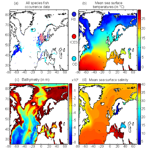
2.3. Materials and Methods? Biological Data Eight species were chosen according to their economic importance, their scientific interest and perhaps more importantly the information available for each of them. Each selected species had a minimum of a least 813 records (Supplementary Table III.1). Some were pelagic, demersal or benthic. Species chosen were (Supplementary Table III.1) (a) Atlantic horse mackerel, (b) European anchovy, (c) European sprat, (d) pollack, (e) common sole, (f) haddock, (g) saithe, and (h) turbot. The Atlantic cod (Gadus morhua L.) was not investigated in this paper as it has been recently described in detail in Beaugrand et al. (submitted) using the same statistical approach and in Bigg et al. (2008) using the model MAXENT (Phillips et al. 2006). Current information on the spatial distribution of these species is presented by Fig. III.S1. They came from two sources: The Food and Agriculture Organization of the United Nations (FAO; http://www.fao.org/fi/figis/maps/compilat.htm) and FishBase (Froese & Pauly 2009; http://www.FishBase.org). More information on the spatial and temporal coverage of the datapoints can be found for each species in Supporting Information (Figs. III.S2 to III.S9). Biological data were uniquely composed of occurrence data (Fig. III.1(a)). These data came from three difference sources: (1) FishBase (Froese & Pauly 2009) using data from the Ocean Biogeographic Information System (OBIS; http://www.iobis.org); (2) ICES-FishMap online atlas ( http://www.ices.dk/marineworld/fishmap/ices/); (3) experts' knowledge. Each occurrence was spatially located (as longitude and latitude) and most of them had information on year. No distinction was made between fish sex and age, and observations retained for the analyses always resulted from catch of post-larval stages and occurrence data taken from 1960 onwards. ? Environmental data A set of environmental data was selected to model the spatial distribution of fish. Annual Sea Surface temperature Annual Sea Surface Temperatures (SST) were chosen because this parameter has strong impacts on a large range of biological processes and on the spatial distribution of marine fish (Tåning 1948; Crisp 1959; Pörtner et al. 2001). This parameter remains relevant for benthic or demersal fish because these species still have a pelagic stage in the life cycle. This larval stage is a critical life cycle phase affecting recruitment (see Cushing 1996). Many studies have shown that the environment exerts its major influence on fish through the effects of temperature on larval development and plankton food availability (e.g. Beaugrand et al. 2003; Drinkwater et al. 2010). Correlation between SST and temperatures at 100 m (data from the World Ocean Atlas 2005; Antonov et al. 2005) was equal to 0.96. The intercept identified by linear regression indicates that we have to subtract 1.85°C from the SST value to achieve the 100 m temperature at the scale of our study. Therefore, at the scale of our study, consideration of temperature at 100m or deeper would not radically affect our conclusions. Observed annual SST from 1960 to 2005 used in this study came from the database International Comprehensive Ocean-Atmosphere Data Set (ICOADS, http://icoads.noaa.gov; Woodruff et al. 1987; Fig. III.1(b)). Forecasted annual SST originated from the ECHAM 4 model (EC for European Centre and HAM for Hamburg; Roeckner et al. 1996). The present data were chosen by the IPCC on the basis of criteria among which are physical plausibility and consistency with global projections. Data utilised here are modelled data based on scenario A2 and B2 (Intergovernmental Panel on Climate Change, 2007b). These data were averaged for two decadal periods: 2050-2059 and 2090-2099. Bathymetry Bathymetry was selected as this parameter strongly influences the potential habitat of marine fish (Louisy 2002). This factor is frequently integrated in ENMs (Hedger et al. 2004; Kaschner et al. 2006). Bathymetric data originated from the global ocean bathymetry map (1° longitude ×1° latitude). The map was constructed from data obtained from ships with detailed gravity anomaly information provided by the satellite GEOSAT and ERS-1 (Smith & Sandwell 1997; Fig. III.1(c)). Figure III.1 : Spatial distribution of both biotic and abiotic data. (a) Spatial distribution of occurrence points for the eight species selected in the study. Points of fish occurrence were reported in blue dots for FishBase (FB), red dots for ICES (ICES) and cyan dots for other sources (OD); each dot represents the occurrence of fish post-larval stages without sex distinction; (b) spatial distribution in the mean sea surface temperature (1960-2005); (c) spatial distribution in the bathymetry; (d) spatial distribution in the annual sea surface salinity (climatology).
Average Sea surface salinity Capacity of dispersal can be modulated by Sea Surface Salinity through the ability of fish to osmoregulate (Schmidt-Nielsen 1990). Annual Sea Surface Salinity (SSS, average values between 0 and 10 meters, Fig. III.1(d)) data were obtained from the Levitus' climatology (Levitus 1982). ICES data ( http://www.ices.dk) were used to complete the Levitus' dataset in coastal regions where there is no assessment of annual SSS (e.g. some regions of the eastern English Channel). ? Statistical procedures Step 1: interpolation of environmental data Both observed and projected annual SST, bathymetry and annual SSS were interpolated linearly on a 0.1°×0.1° spatial grid to fit more closely the coasts on the maps. The spatial domain ranged from 110°W to 70.5°E and from 50°S to 90°N. However, only the part of the North Atlantic ranging from 80°W to 70.5°E and from 25°N to 85°N was investigated for fish spatial projections. This represented a total of 2,530,206 geographical cells. Step 2: attribution of environmental parameters at each fish occurrence point The environmental stratum (i.e. the combination of three environmental parameters or triplet; Guisan & Zimmermann 2000) for each occurrence point and each fish were recovered from the environmental datasets. When the date of an observation was unknown, an average was used for the time period 1960-2005 to attribute a mean environmental combination at the geographical location. This average is unlikely to affect strongly the thermal niche of the species, which is much more influenced by the spatial than the temporal variance in SST (Beaugrand et al. 2008). In the same way, when the date of trawl or observation was available in the form of a time period (e.g. catch data from 1985 to 1995), the environmental stratum was averaged for this time period. This pre-processing of the data led to eight matrices (we called training sets or reference matrices Zn,p), one matrix per species, each having n observations with three environmental parameters (see Supplementary Table III.1 for the values of n for each species; p=3). Step 3: corrected training set The ENM uses the above matrices to evaluate the probability of occurrence of each species. However, as they stand, the reference matrices could be biased towards regions more investigated than others due to concentration of fishing activities or scientific campaigns. To consider this potential drawback, the reference matrices were corrected prior to the application of the model. This procedure was similar to what is performed in the programme RASTERIZ included in the GARP Modelling System (GMS; Stockwell & Peters 1999) and was implemented to give the same weight to regions of small or massive occurrence densities. A three-dimensional matrix was defined. The first dimension, reflecting SST, varied between 0°C and 30°C with an increment of 1°C. The second dimension, integrating bathymetry, ranged between 0 and 6000m with a resolution of 10 m. The third dimension, for SSS, extended from 0 to 40 with an increment of 2. Each cell of the matrix could be considered as a class of environmental stratum. When data were present in a stratum, the stratum was kept for further analyses. This procedure eliminated the potential effect of the concentration of sampling in an area (Beaugrand et al. submitted). After having applied the procedure, the matrices Zn,p become Zm,p with m=n. Step 4: representation of the ecological niche of each species An important assumption in most ENMs used to model the potential species habitat is to have beforehand correctly determined the contour(s) of the ecological niche of the species (Lacoste & Salanon 2001). Many ENMs are based on the Hutchinson's concept (Hutchinson, 1957) of the ecological niche. Hutchinson (1957) defined the niche of a species as a multidimensional envelop of environmental factors in which the species is capable to maintain its population. As the niche is often inferred from the spatial distribution of organisms, ENMs assess the realised niche (Helaouët & Beaugrand 2009). When the niche is incompletely estimated, most ENMs fail to give a reliable modelling of the potential distribution. Estimating the ecological niche of a species can be made in different ways (Soberón & Peterson 2005). Here we used the environmental triplets (i.e. the environmental conditions where the species were detected) to model the spatial distribution of each species. Step 5: calculation of the probability of fish occurrence An increasing number of ENMs has been recently developed to model the spatial distribution of species and forecast potential modification in the context of global climate change (Guisan & Zimmermann 2000; Thuiller 2003; Austin 2007). Here, we used the Non-Parametric Probabilistic Ecological Niche model (NPPEN) recently developed and described in details by Beaugrand et al. (submitted). The model tests whether or not an observation (i.e. the j geographical cells of our environmental grids; j=2,530,206), characterised by an environmental stratum (p variables; p=3), belongs to a reference matrix, here matrix Zm,p. Mathematically, the technique is nonparametric using a modified version of the Multiple Response Permutation Procedure (MRPP; Mielke et al. 1981). The technique utilises the Generalised Mahalanobis distance (Mahalanobis 1936), which enables the correlation between variables to considered (Farber & Kadmon 2003). The distance was therefore calculated as follows:
With x the vector of length p, representing
the values of the three environmental triplets to be tested
(j=2,530,206), Rp,p the correlation matrix of
reference matrix Zm,p and Figure III.2 : Ecological niches estimated after hoogenization (i.e. correction) of the original training set according to three environmental parameters: sea surface temperature (SST, left panels), bathymetry (middle panels) and sea surface salinity (SSS, right panels). (a) Atlantic horse mackerel, (b) European anchovy, (c) European sprat, (d) pollack, (e) common sole, (f) haddock, (g) saithe and (h) turbot. The number of observations was log10 transformed for bathymetry.
To calculate the probability of significance of the distance, each observation of the reference matrix Zm,p was permuted to become the observation to be tested and the original tested observation was included to the reference matrix. The Mahalanobis generalised distance was then recalculated for each permutation. The number of total permutations was equal to m. A probability w can then be assessed by looking at the number of times the simulated distance was found to be superior or equal to the observed distance between the observation and the reference matrix Zm,p. The probability was calculated as follows:
Where the probability w was the number of times the simulated Mahalanobis generalised distance ds was found to be superior or equal to the observed mean distance do. When w tends towards 1, the observation has environmental conditions that represent the centre of the species niche. When w tends towards 0, the observation has environmental conditions outside the species niche. It is important to have a large reference matrix Zm,p so that the resolution of the probability is as high as possible. Such a procedure was performed for each of the j=2,530,206 observations and all 8 species. Step 6: Evaluation of the model as a function of different simulated training sets The model can be used to assess the ecological niche of a species. Before calculating the spatial pattern of changes in the probability of fish occurrence, we evaluated how the model reacted to different kind of simulated training sets: (1) homogeneous (considered here as the set of reference); (2) nearly-homogeneous; (3) symmetrical bimodal; (4) asymmetrical bimodal (see Fig. III.3), therefore simulating some observed ecological niches (see Fig. III.2). The mean difference D between the set of reference R and the simulated training set S was assessed as follows:
With 0=D=1, n the number of probabilities to be compared, Ri the ith probability of the set of reference and Si the ith probability of the simulated training set.
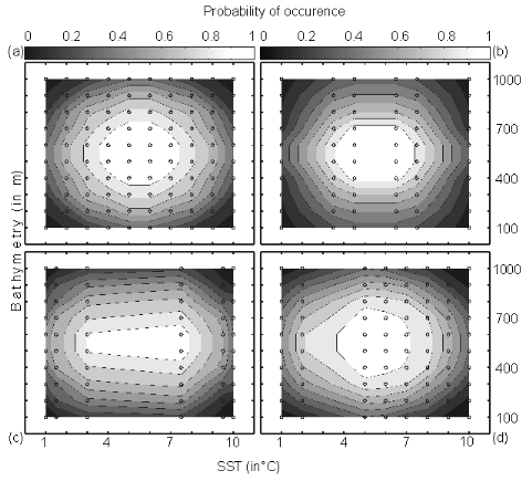
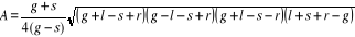
Step 7: Application of the model for different sets of environmental conditions The model was then applied on the corrected training set (see Step 3) with as environmental variables, the bathymetry and annual SSS (assumed to be constant over the period) and both observed and projected annual SST. Spatial distributions (see Figs. III.4 and III.S12 to III.S19) were provided for the period 1960-1969, the period 2000-2005 (observed SST data) and the decades 2050s and 2090s (projected SST data, see Fig. III.S11 to III.S19). Step 8: Statistical analyses of the results Comparison of the models NPPEN and AquaMap Figure II. 3 For each species, a correlation analysis was applied to compare the maps of probability of fish occurrence inferred from the AquaMap approach of Kaschner and colleagues (a modified version of the Relative Environmental Suitability model of Kaschner et al. 2006) and the model NPPEN. This comparison was performed on maps based on annual SST averaged for the period 1960-2005. To evaluate the impact of spatial autocorrelation when the correlation was calculated between maps, the minimum degree of freedom needed to have a significant correlation (p=0.05) was also assessed (Beaugrand & Helaouët 2008). Figure III.3 : Probability of occurrence calculated using NPPEN from two variables (bathymetry and annual sea surface temperature (SST). (a) Reference training set with occurrence points (as circle) and associated probability (shaded grey), (b) simulated training set 1 (central gap in occurrence points), (c) simulated training set 2 (large central gap and slight asymmetry in occurrence points) and (d) simulated training set 3 (pronounced asymmetry in occurrence points). Quantification of long-term changes in potential species distribution To quantify the potential long-term changes in species distribution, probabilities of occurrence for the periods 1960-1969, 2000-2005 and 2090-2099 (scenarios A2 and B2) were converted into binary data. The presence was considered as certain when the probability of occurrence for a species was =0.2 (threshold selected by trial and error; different thresholds were selected and gave similar conclusions) and a value of 1 was attributed. Below this threshold, a 0 was ascribed. The differences between the 2000-2005 and 1960-1969 and the period 2090-2099 (for scenarios A2 and B2) and 1960-1969 were then calculated. A positive difference (quantified in km²) was interpreted as a gain of potential habitat and inversely. The surface A was calculated by assimilating the geographical cell to an isosceles trapeze:
With g being the longitudinal distance (in km) between the two minimum latitudes of the trapeze, s the longitudinal distance (in km) between the two maximum latitudes of the trapeze, l the distance between the maximum and minimum latitude on the western part of the trapeze and r the distance between the maximum and minimum latitude on the eastern part of the trapeze. The four distances were assessed as follows (Beaugrand & Ibañez, 2002): d(i,j)=6377.221 x hi,j (5) With di,j being the geographical distance between point i and j, the constant the Earth radius and hi,j computed as follows (Beaugrand & Ibañez 2002):
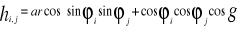
With öi the latitude (in radians) at point i, öj the latitude (in radians) at point j and g the difference in longitude between i and j. |
|


 (1)
(1) the average environmental condition inferred from
Zm,p. There were as many calculations of the
Mahalanobis generalised distance as environmental triplets to be tested
(j=2,530,206). These triplets were chosen in such a way to cover the entire
ecological niche of the species or its entire spatial distribution (see Figs.
III.S1, III.1 and III.4). Many ecological niche models are based on the
Mahalanobis generalised distance (Farber & Kadmon 2003; Calenge et
al. 2008; Nogués-Bravo et al. 2008). However, the novelty
lies in the fact that the model offers a new way to calculate the probability
of the Mahalanobis generalised distance using a non parametric procedure.
the average environmental condition inferred from
Zm,p. There were as many calculations of the
Mahalanobis generalised distance as environmental triplets to be tested
(j=2,530,206). These triplets were chosen in such a way to cover the entire
ecological niche of the species or its entire spatial distribution (see Figs.
III.S1, III.1 and III.4). Many ecological niche models are based on the
Mahalanobis generalised distance (Farber & Kadmon 2003; Calenge et
al. 2008; Nogués-Bravo et al. 2008). However, the novelty
lies in the fact that the model offers a new way to calculate the probability
of the Mahalanobis generalised distance using a non parametric procedure. 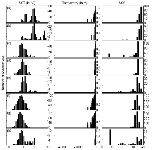
 (2)
(2) (3)
(3)
 (4)
(4) (6)
(6)