Impact du réchauffement climatique sur la distribution spatiale des ressources halieutiques le long du littoral français: observations et scénarios( Télécharger le fichier original )par Sylvain Lenoir Université Lille 1 Science - Doctorat 2011 |

2.5. DiscussionOur use of an ENM to determine the potential geographical range of a species excludes fundamental biotic interactions or processes related to resource availability. Indeed, process models enable physiological constraints, population dynamics, life history traits and trophic interactions to be considered (Speirs et al. 2006). However, such detailed knowledge is rarely available (Carpenter et al. 1993). The large scale at which our study was conducted overcomes partly this drawback, trophic interactions being for example more important at a local scale (Pearson & Dawson 2003). We chose to base our projections on a limited number of parameters for the following reasons: (1) too many parameters increase the risk of multicollinearity, which could prevent the calculation of the Mahalanobis generalised distance; (2) the number of samples needed in the reference matrix increases when the number of parameters augments; (3) A high number of parameters would also increase the uncertainties of the model. We did not consider habitat characteristics (e.g. sediment type), essential for common sole and turbot. Indeed, it was assumed that climate exerts its major influence on fish through the effects of temperature on larval development since the larval stage is a critical life cycle phase affecting recruitment (Cushing 1996). Although adult species selected in this study are pelagic, demersal or benthic, all have a pelagic stage. Therefore, our result should be more interpreted as reflecting the potential habitat of a species, without the influence of the type of sediments (Amara et al. 2004) or processes such as trophic interactions or dispersal (Pulliam 2000). It should be reminded that the optimal part of the realised niche (sensu Hutchinson, 1957) was inferred from the frequency of occurrence of each species in a particular stratum. A clear assumption in our technique, as in other modelling techniques based on presence-only data, is that the maximum frequency of occurrence occurs at the optimal part of the realised niche. It is thereby expected that a too scarce sampling may deform the realised niche and bias our projection. This is the reason why we based on projection on a large number of datapoints (Supplementary Table III.1) and represented the realised niche of all species to examine if the whole niche was covered (Figs. III.S10 and III.2). Furthermore, the technique is not sensitive to spatial scarcity of the data but rather to an incomplete assessment of the preferendum of a species. We have to know sufficiently well the niche to project the spatial distribution of the species. The quality of the data is a fundamental parameter affecting the dependability of results of ENMs (Stockwell & Peterson 2002). Contrary to the terrestrial realm, the marine biosphere is more difficult to sample and the joint information on presence and absence is rare. Therefore, ENMs requiring presence/absence data such as Generalised Additive Models (GAM; Hastie & Tibshirani 1990) or Generalised Linear Models (GLM; McCullagh & Nelder 1983) although representing powerful tools and often producing better predictions than presence-only evaluators (Brotons et al. 2004) are inappropriate. Ecological Niche Factor analysis (ENFA; Hirzel 2001), AquaMap (Kaschner et al. 2006), the maximum entropy modelling (MAXENT; Phillips et al. 2006), BIOCLIM, HABITAT and DOMAIN are some of the techniques applied when only-presence data are available (Carpenter et al. 1993). The comparison of the model NPPEN with the one of Kaschner et al. (2006) indicated that although for some species the correlation was high (see Table III.1), substantial differences might occur for some species (e.g. European anchovy and pollack). Such differences may be related to the inherent property of the model (e.g. the difference of objectivity between the two techniques), the number and the choice of the environmental parameters or the number of samples (see the correlations between the two models and the number of samples) to have a representative training set. AquaMap is more dependent on expert knowledge and the contour of the trapezoidal model is often fixed from biological expertise. One of the main advantages of the technique NPPEN is that it is nonparametric, contrary to ENFA (Hirzel et al. 2006), does not require the selection of underlying functions as in MAXENT (Phillips et al. 2006) and parametrisation or the attribution of thresholds as in AquaMap (Kaschner et al. 2006), ENFA and MAXENT. However, the analysis is dependent, as most of the current available techniques, upon a correct assessment of the ecological niche and is highly dependent of the quality of the training set (especially the contour of the niche, see Fig. III.3). A too high number of outliers might have a strong influence on probability (Beaugrand et al. submitted). This drawback can be overcome by the use of the procedure of homogenisation with an increasing threshold (threshold of presence data in an environmental stratum=2). However, caution is needed as the homogenisation can lead to an underassessment of the width of the niche. The probability from our model is unlikely to have been strongly influenced by spatial autocorrelation (SAC; Segurado et al. 2006; Dormann 2007), likely to occur in environmental parameters such as annual SST. Spatial autocorrelation increases the Type I error rate which leads to the incorrect rejection of the null hypothesis of no effect. SAC is likely to affect more strongly regression techniques such as GLMs and GAMs and some adjustments are being developed to overcome this problem (Dormann et al. 2007). However, the impact of SAC remains uncertain for some authors (Diniz-Filho et al. 2003). The determination of SAC was not undertaken in this study. However, the step of homogenisation (or adjustment of the training set) we applied in this study have probably strongly limit the influence of SAC on probability. Such procedure, which reduces pseudo-replication, is congruent with recommendations of some authors (Brito et al. 1999; Stockwell & Peters 1999; Guisan & Zimmermann 2000; Segurado et al. 2006). The influence of climate change on marine ecosystems and more particularly on species distribution has become prominent (Intergovernmental Panel on Climate Change 2007a). In this context, there is an urgent need to better assess the spatial distribution of species for conservation and management issues (Parmesan 2006). The new model NPPEN was used to estimate the past, current and potential future changes in species distribution of some marine fish commercially exploited in the North Atlantic sector. The new maps of spatial distribution provide quantitative information on spatial distribution often presented as categorical or binary maps (FAO; http://www.fao.org/fi/figis/maps/compilat.htm and (Louisy 2002). The new model also gives alternative views on quantitative spatial distribution recently provided by Cheung et al. (2008a, 2008b, 2009) using a new dynamic bioclimate envelope model or by the method AquaMap (Kaschner et al. 2006) used in FishBase (Froese & Pauly 2009). One important assumption when modelled SST data is that there is no discrepancy between observed SST (ICOADS) and modelled SST (ECHAM 4). Beaugrand et al. (2008) compared observed ICOADS and ECHAM 4 modelled data for the period 1990-2005. Modelled and observed data on annual SST were highly positively correlated in the area covered by this study (r=0.95, p<0.0001, n=1809), showing that the model ECHAM 4 captures relatively well the complexity of the hydro-climatic environment of the North Atlantic at a decadal scale. All modelled spatial distributions explain current observed large-scale changes in fish distribution (e.g. Perry et al. 2005; Rose 2005; Kirby et al. 2006; Hiddink & Ter Hofstede 2008; Cheung et al. 2008b, 2009). Overall, results show a migration of marine resources polewards at rate varying among species, agreeing with other studies based on observational data (Quero et al. 1998; Brander et al. 2003; Perry et al. 2005; Kirby et al. 2006). Northward movements are clearly detected for most species with potential habitat gained at the northern edge of the spatial distribution and potential habitat lost at their southern edge. Brander (2003) also noted this northward movement for commercial gadoid and flatfish. They found however some examples of southward shifts that he explained by local hydrodynamical characteristics (e.g. sardine in upwelling regions off Portugal). Furthermore, Perry et al. (2005) investigating long-term spatial changes in 36 species found that about two-thirds of both commercial and non-commercial species shifts their spatial distribution northwards in the North Sea as a response to sea temperature warming. The authors observed that some species moved in deeper regions, suggesting that some species may adapt to temperature warming by moving vertically. This effect was not accounted for in our statistical model. Perhaps more interestingly, our results indicate that some species may not be able to track their environmental envelop and could loss a significant amount of their habitats (Fig. III.5 and Table III.2: pollack) as they might be restricted by other specific local or regional constraints related to the bathymetry (e.g. flatfish). Of some interests, the model explains the pronounced increase in the abundance of European sprat in the Baltic Sea and the North Sea since the 1990s, which has had some influence on some seabird species (Österblom et al. 2008; Wanless et al. 2005). For example, the increase in the stock of European sprat in the Baltic Sea has led to a decrease in energetic content (Österblom et al. 2006). These authors showed how this loss in quality food caused loss in fledging mass of common guillemot chicks. Our model could be applied on sandeels to examine whether a decrease in the probability of occurrence of this species paralleled the increase in European sprat. Our results show that the general latitudinal movement in fish distribution detected for past decades may accelerate (Fig. III.S11, Table III.2). More sustained warming could trigger more rapid northward shifts. Associated with fishing, climate-induced shifts could have a strong impact on socio-economical systems by precipitating the collapse of some stocks, especially at the southern edge of current species distribution (Beaugrand et al. 2008). Other regions (e.g. the Barents Sea) will see a pronounced increase in their potential habitat. However, relaxed fishing pressure due to an improved ecosystem carrying capacity might mitigate the potential for growth in fish stocks (e.g. gadoids in the Barents Sea). The uncertainties related to these projections are obviously high and perhaps more importantly cannot at present be assessed with confidence. These uncertainties are related to the climatic scenario itself (scenario A2 and B2), the uncertainties of the physical model (here the ECHAM 4 model) and limitations of our own model. Many other uncertainties remain and the complexity of the system makes it difficult to consider these maps as exact predictions but rather as projections of potential distribution in the absence of biotic interactions, dispersal and processes related to population dynamics which cannot be realistically considered with our current level of knowledge. Nevertheless, ENMs might provide a new management tool against which changes in the resource might be better anticipated and improve sustainable exploitation strategy in the context of rapid global climate change associated to pronounced anthropogenic impact on the marine biosphere. Acknowledgments We are grateful to all past and present members and supporters of the FishBase website ( http://www.FishBase.org), whose continuous efforts have allowed the establishment of the fish data set. We thank Dr Keith Brander for helpful comments on an early version of the manuscript. The research was supported by the French Agency of Research and Technology (ANRT, grant CIFRE 862/2007).
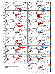
Figure III.S1 : Spatial distribution of species selected in this study inferred from the FAO geographical distribution model (left) and the AquaMap approach (right, Kaschner et al., 2006). (a) Atlantic horse mackerel, (b) European anchovy, (c) European sprat, (d) pollack, (e) common sole, (f) haddock, (g) saithe and (h) turbot. The FAO model illustrates the predicted distribution area of marine fish from a GIS approach. Red areas represent regions where the presence of the species is considered as certain. No FAO map for turbot was available. The RES model represents the probability of species presence (between 0 and 1).
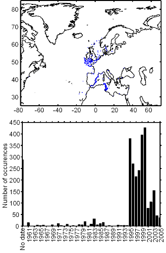
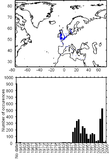
Figure III.S2 : Spatial and temporal distribution of occurrences datapoints for Atlantic horse mackerel used to assess the spatial distribution of species.
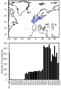
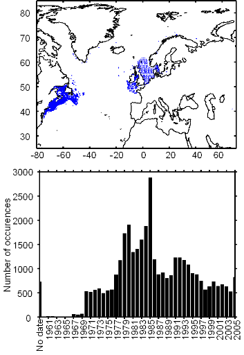
Figure III.S3 : Spatial and temporal distribution of occurrence datapoints for European anchovy used to assess the spatial distribution of species.
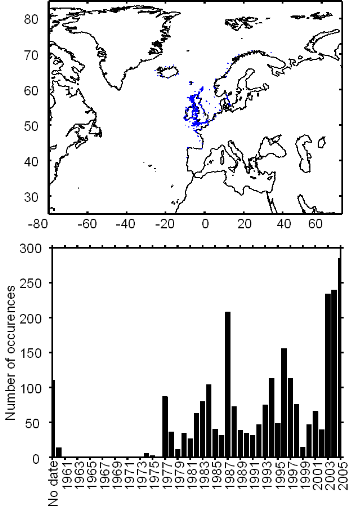
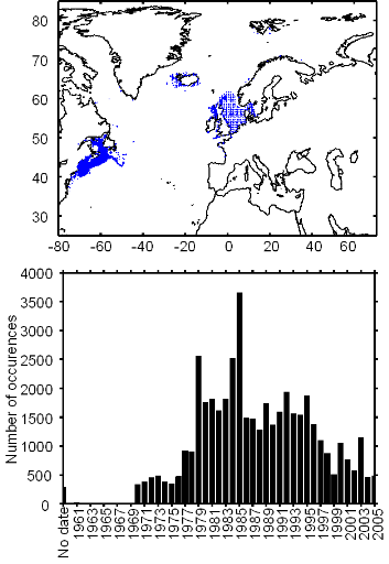
Figure III.S4 : Spatial and temporal distribution of occurrence datapoints for European sprat used to assess the spatial distribution of species.
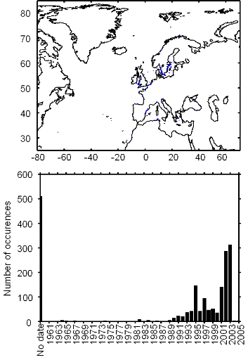
Figure III.S5 : Spatial and temporal distribution of occurrence datapoints for pollack used to assess the spatial distribution of species.
Figure III.S6 : Spatial and temporal distribution of occurrence datapoints for common sole used to assess the spatial distribution of species.
Figure III.S7 : Spatial and temporal distribution of occurrence datapoints for haddock used to assess the spatial distribution of species.
Figure III.S8 : Spatial and temporal distribution of occurrence datapoints for saithe used to assess the spatial distribution of species.
Figure III.S9 : Spatial and temporal distribution of occurrence datapoints for turbot used to assess the spatial distribution of species.
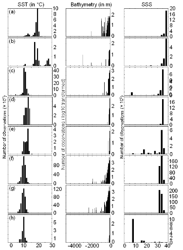
Figure III.S10 : Ecological niches (sensu Hutchinson 1957) estimated from the occurrence data of the original (uncorrected) training set and as a function of three environmental parameters: annual sea surface temperature (SST, left panels), bathymetry (middle panels) and annual sea surface salinity (SSS, right panels). (a) Atlantic horse mackerel, (b) European anchovy, (c) European sprat, (d) pollack, (e) common sole, (f) haddock, (g) saithe and (h) turbot.
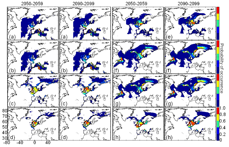
Figure III.S11 : Estimated probability of occurrence using the model NPPEN for the decade 2050-2059 and 2090-2099 (scenario B2) in the North Atlantic Ocean. (a) Atlantic horse mackerel, (b) European anchovy, (c) European sprat, (d) pollack, (e) common sole, (f) haddock, (g) saithe and (h) turbot. The western boundary of the model was fixed to 401W. This was arbitrary selected for species (but haddock and saithe) which are only found on the eastern side of the Atlantic Ocean.
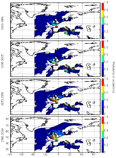
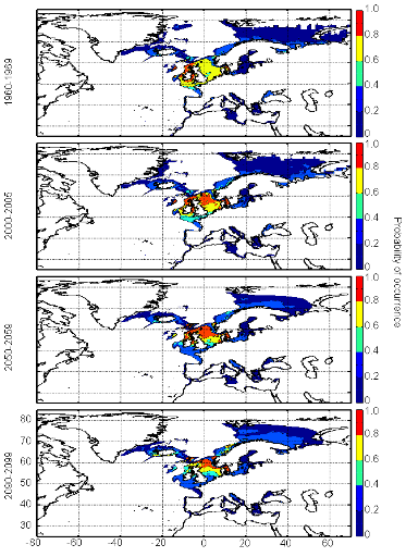
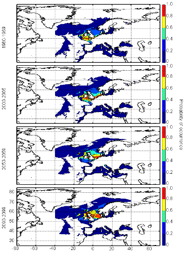
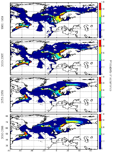
Figure III.S12 : Estimated probability of occurrence of Atlantic horse mackerel using the model NPPEN for the decade 1960-1969, the time period 2000-2005 and for the decades 2050-2059 and 2090-2099 (scenario B2) in the North Atlantic Ocean.
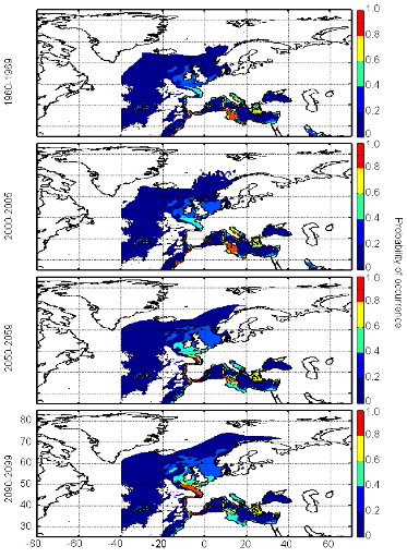
Figure III.S13 : Estimated probability of occurrence of European anchovy using the model NPPEN for the decade 1960-1969, the time period 2000-2005 and for the decades 2050-2059 and 2090-2099 (scenario B2) in the North Atlantic Ocean.
Figure III.S14 : Estimated probability of occurrence of European sprat using the model NPPEN for the decade 1960-1969, the time period 2000-2005 and for the decades 2050-2059 and 2090-2099 (scenario B2) in the North Atlantic Ocean.
Figure III.S15 : Estimated probability of occurrence of pollack using the model NPPEN for the decade 1960-1969, the time period 2000-2005 and for the decades 2050-2059 and 2090-2099 (scenario B2) in the North Atlantic Ocean.
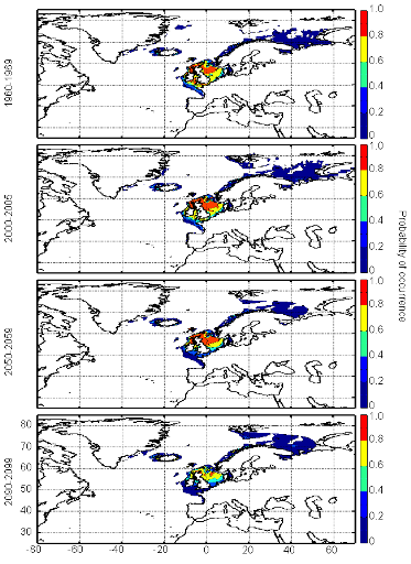
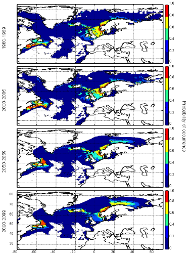
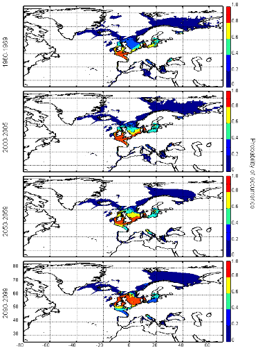
Figure III.S16 : Estimated probability of occurrence of common sole using the model NPPEN for the decade 1960-1969, the time period 2000-2005 and for the decades 2050-2059 and 2090-2099 (scenario B2) in the North Atlantic Ocean.
Figure III.S17 : Estimated probability of occurrence of haddock using the model NPPEN for the decade 1960-1969, the time period 2000-2005 and for the decades 2050-2059 and 2090-2099 (scenario B2) in the North Atlantic Ocean.
Figure III.S18 : Estimated probability of occurrence of saithe using the model NPPEN for the decade 1960-1969, the time period 2000-2005 and for the decades 2050-2059 and 2090-2099 (scenario B2) in the North Atlantic Ocean.
Figure III.S19 : Estimated probability of occurrence of turbot using the model NPPEN for the decade 1960-1969, the time period 2000-2005 and for the decades 2050-2059 and 2090-2099 (scenario B2) in the North Atlantic Ocean. TableIII.S1 : List of marine fish species used in this study with their official FAO and scientific names. The bathymetric preference for each species was obtained from Louisy (2002) and FishBase (Froese & Pauly, 2009; http://www.FishBase.org). The number of occurrence points before (left) and after (right) the attribution of environmental variables is indicated, showing the reduction in the data because of missing environmental data.
Supplementary Table III.1 Lenoir et al. |
|