Memoire Online - Forest degradation, a methodological approach usingremote sensing techniques: literature review

Forest degradation, a methodological approach using remote sensing techniques: Literature Review

0. Introduction

Forest degradation is a serious problem, environmentally, socially and economically particularly in developing countries. It is estimated that as much as 850 million hectares (ITTO, 2002) of forests and forest lands are degraded. Yet it is difficult to quantify the scale of the problem since at national and sub-national levels forest degradation is perceived differently by the various stakeholders who have different objectives.

Forest degradation has adverse impacts on forest ecosystems and on the goods and services they provide. Many of these goods and services are linked to human well-being and some to the global carbon cycle and thus to life on Earth.

Policy makers and forest managers need information on forest degradation. They need to be able to monitor changes happening in forests. They need to know where forest degradation is taking place, what causes it and how serious the impacts are in order to prioritize the allocation of scarce human and financial resources to the prevention of degradation and to the restoration and rehabilitation of degraded forests. (Simula , 2009).

In addition, reviewing on forest degradation is required to demonstrate efforts to tackle the problem and meet global objectives and targets. The proposed new Biodiversity Target includes a target on reduction of forest degradation. The agreement to establish a mechanism under the UNFCCC aimed at reducing emissions from deforestation and forest degradation (REDD) in developing countries has added a political dimension and the potential availability of substantial funds to reward developing countries that manage to reduce the level of forest degradation.

Accurate and up-to-date land use/cover assessments are important to define natural resource management strategies and policies for conservation especially in forest areas. Understanding the causes and consequences of land cover change and their cascading effects on many components of functional ecosystems, are the case for identifying negative effects on biological resources and human development ( Bicheron et al,2008; Bunker et al, 2005).

Satellite remote sensing provides a meaningful method for detecting vegetation or land cover changes (Smith et al, 2004). Changes in the composition and spatial distribution of forest cover are a major environmental concern, affecting many biological, biochemical and ecological processes. Remotely sensed data are widely used to understand and manage environmental resources by determining land cover/use changes such as quantification of forest degradation. By comparing the images taken in different times, the changes in landscape level can be easily detected. Monitoring land cover and land cover change at regional and global scales often requires sensors data to identify and map landscape features and patterns with sufficient detail (

Defries et al., 2001).Detailed and updated resource inventories are needed to support land use planning and sustainable management .

This literature review addresses how remote sensing techniques can be used to assess forest degradation directly or indirectly by mean of different type of degradation process occurring in the forest area.

1. Remote Sensing, an Overview

1.1. Definitions

Remote sensing can be defined as learning something about an object without touching it. As human beings, we remotely sense objects with a number of our senses including our eyes, noses, and ears. ( Cogalton,2010); for Thomas et al.(2004) ,remote sensing is the science and art of obtaining information about an object, area, or phenomenon through the analysis of data acquired by a device that is not in contact with the object, area or phenomenon under investigation.

The field of remote sensing can be divided into two general categories: analog remote sensing and digital remote sensing. Analog remote sensing uses film to record the electromagnetic energy. Digital remote sensing uses some type of sensor to convert the electromagnetic energy into numbers that can be recorded as bits and bytes on a computer and then displayed on a monitor.

1.1.1. Analog remote sensing

The field of analog remote sensing can be divided into two general categories: photointerpretation and photogrammetry. Photo interpretation is the qualitative or artistic component of analog remote sensing. Photogrammetry is the science, measurements, and the more quantitative component of analog remote sensing. Both components are important in the understanding of analog remote sensing

1.1.2. Digital Remote Sensing

While analog remote sensing has a long history and tradition, the use of digital remote sensing is relatively new and was built on many of the concepts and skills used in analog remote sensing. Digital remote sensing effectively began with the launch of the first Landsat satellite in 1972. Since the launch of Landsat 1, there have been tremendous strides in the development of not only other multispectral scanner systems, but also hyperspectral and digital camera systems. However, regardless of the digital sensor there are a number of key factors to consider that are common to all. For Campbell ,(2007) these factors include:

Spectral resolution is typically defined as the number of portions of the electromagnetic spectrum that are sensed by the remote sensing device. These portions are referred to as «bands.»A second factor that is important in spectral resolution is the width of the bands. Traditionally, the band widths have been quite wide in multispectral imagery, often covering an entire color (e.g., the red or the blue portions) of the spectrum. If the remote sensing device captures only one band of imagery, it is called a panchromatic sensor and the resulting images will be black and white, regardless of the portion of the spectrum sensed. More recent hyperspectral imagery tends to have much narrower band widths with several to many bands within a single color of the spectrum.

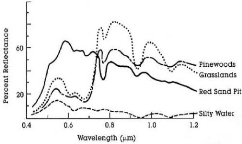
Figure 1 comparison of spectrums of vegetation,bare soil,snow and water, in Asner et al,2004 - Spatial Resolution

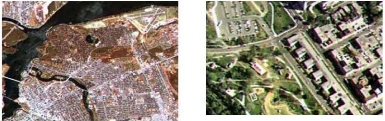
Spatial resolution is defined by the pixel size of the imagery. A pixel or picture element is the smallest two-dimensional area sensed by the remote sensing device. An image is made up of a matrix of pixels. The digital remote sensing device records a spectral response for each wavelength of electromagnetic energy or «band» for each pixel. This response is called the brightness value (BV) or the digital number (DN). In Cogalton, 2009; the range of brightness values depends on the radiometric resolution. If a pixel is recorded for a homogeneous area then the spectral response for that pixel will be purely that type. However, if the pixel is recorded for an area that has a mixture of types, then the spectral response will be an average of all that the pixel encompasses. Depending on the size of the pixels, many pixels may be mixtures.

Figure 2 : Spatial resolution of different types of sensors, respectively for spot and Ikonos in Canada center for remote sensing CCRS,2003

The numeric range of the brightness values that records the spectral response for a pixel is determined by the radiometric resolution of the digital remote sensing device. These data are recorded as numbers in a computer as bits and bytes (Jensen, 2007). A bit is simply a binary value of either 0 or 1 and represents the most elemental method of how a computer works. If an image is recorded in a single bit then each pixel is either black or white. No gray levels are possible. Adding bits adds range. If the radiometric resolution is 2 bits, then 4 values are possible (2 raised to the second power = 4). The possible values would be 0, 1, 2, and 3. Early Landsat imagery had 6-bit resolution (2 raised to the sixth power = 64) with a range of values from 0 to 63. Most imagery today has a radiometric resolution of 8 bits or 1 byte (range from 0 to 255). Some of the more recent digital remote sensing devices have 11 or even 12 bits.

Temporal resolution is defined by how often a particular remote sensing device can image a particular area of interest. Sensors in airplanes and helicopters can acquire imagery of an area whenever it is needed. Sensors on satellites are in a given orbit and can only image a selected area on a set schedule. Landsat is a nadir sensor; it only images perpendicular to the Earth's surface, and therefore can only sense the same place every 16 days. Other sensors are pointable and can acquire off-nadir imagery.

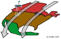
Figure 3 : temporal resolution movement of a sensor in CCRS, 2003 Table 1 Digital characteristics of some satellite are given below, personal compilation

satellite	sensor	Ground resolution	Radiometric resolution	Temporal resolution
landsat	MSS	80m	-	18 days
landsat	Thematic Mapper	30 m	6 bit	16 days
Spot	XS(multispectral)	20 m	6 bit	6 days
spot	panchromatic	10 m	6 bit	5 days
Ikonos	Multispectral	4 m	11 bit	2,9 days

1.2. Digital image analysis

Digital image analysis in digital remote sensing is analogous to photo interpretation in analog remote sensing. It is the process by which the selected imagery is converted/processed into information in the form of a thematic map. Digital image analysis is performed through a series of steps. These steps include: (1) image acquisition/selection, (2) pre-processing including image enhancement, (3) classification, (4) post-processing, and (5) accuracy assessment.

1.2.1. Image Acquisition/Selection

Selection or acquisition of the appropriate remotely sensed imagery is foremost determined by the application or objective of the analysis and the budget. Once these factors are known, the analyst should answer the questions presented previously. These questions include: what spectral, spatial, radiometric, temporal resolution and extent are required to accomplish the objectives of the study within the given budget? Once the answers to these questions are known, then the analyst can obtain the necessary imagery either from an archive of existing imagery or request acquisition of a new image from the appropriate image source.

1.2.2. Pre-processing

Pre-processing is defined as any technique performed on the image prior to the classification. There are many possible pre-processing techniques. However, three of the most important techniques include: geometric registration, radiometric/ atmospheric correction, and numerous forms of image enhancement.

1.2.3. Classification

Classification of digital data has historically been limited to spectral information (tone/color). While these methods attempted to build on the interpretation methods developed in analog remote sensing, the use of the other elements of photo interpretation beyond just color/tone has been problematic. In addition, digital image classification has traditionally been pixel based. A pixel is an arbitrary sample of the ground and represents the average spectral response for all objects occurring within the pixel. The earliest classification techniques tended to mimic photo interpretation and were called supervised classification techniques..

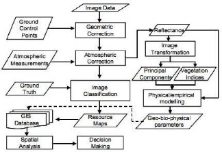
Figure 4 : A schematic diagram of general image processing procedures, Campbell, 2007

1.2.3.2. Combined Approaches.

Many remote sensing scientists have attempted to combine the supervised and unsupervised techniques together to take the maximum advantage of these two techniques while minimizing the disadvantages. Many of these examples can be found in the literature. A technique by Jensen (2005)

1.2.3.3. Advanced Approaches.

Using supervised or unsupervised classification approaches only work moderately well. Even the combined approaches only improve our ability to create accurate thematic maps a little more than using each technique separately. Therefore, a large amount of effort has been devoted to developing advanced classification approaches to improve our ability to create accurate thematic maps from digital remotely sensed imagery. While there are many advanced approaches, this paper will only mention three: (1) classification and regression tree (CART) analysis; (2) artificial neural networks (ANN); and (3) support vector machines (SVM).

1.2.3.4. Object-Based Approaches ( polygon approach)

By far the greatest advance in classifying digital remotely sensed data in this century has been the widespread development and adoption of object-based image analysis (OBIA). Traditionally, all classifications were performed on a pixel basis. Given that a pixel is an arbitrary delineation of an area of the ground, any selected pixel may or may not be representative of the vegetation/land cover of that area. (Gamanya et al.,2008) In the OBIA approach, unlabeled

pixels are grouped into meaningful polygons that are then classified as polygons rather than individual pixels. This method increases the number of attributes such as polygon shape, texture, perimeter to area ratio, and many others that can be used to more accurately classify that grouping of pixels (Blaschke et al., 2008).

1.2.4. Post-processing

Post-processing can be defined as those techniques applied to the imagery after it has been through the classification process--in other words, any techniques applied to the thematic map. It has been said that one analyst's pre-processing is another analyst's post-processing. It is true that many techniques that could be applied to the digital imagery as a pre-processing step may also be applied to the thematic map as a post-processing step. This statement is especially true of geometric registration. While currently most geometric correction is performed on the original imagery, such was not always the case. Historically, to avoid resampling the imagery and potentially removing important variation (information), the thematic map was geometrically registered to the ground instead of the original imagery (Jensen, 2005).

1.2.5. Accuracy Assessment

Accuracy assessment is a vital step in any digital remote sensing project. The methods summarized here can be found in detail in Green et al., (2009). Historically, thematic maps generated from analog remotely sensed data through the use of photo interpretation were not assessed for accuracy. However, with the advent of digital remote sensing, quantitatively assessing the accuracy of thematic maps became a standard part of the mapping project.

Once the error matrix is generated, some basic descriptive statistics including overall, producer's, (Cogalton, 2010) and user's accuracies can be computed. In addition, there are a number of analysis techniques that can be performed from the error matrix. Most notable of these techniques is the Kappa analysis, which allows the analyst to statistically test if one error matrix is significantly different than another.

1.3. Digital Image Types 1.3.1. Multispectral Imagery

The dominant digital image type for the last 40 years has been multispectral imagery, from the launch of the first Landsat in 1972 through the launch of the latest GeoEye and DigitalGlobe sensors.(Tucker,1985) Multispectral imagery contains multiple bands (more than 2 and less than 20) across a range of the electromagnetic spectrum. While there has been a marked increase in spatial resolution, especially of commercial imagery, during these 40 years it should be noted that there continues to be a great demand for mid-resolution imagery.

1.3.2. Hyperspectral Imagery

Hyperspectral imagery is acquired using a sensor that collects many tens to even hundreds of bands of electromagnetic energy. This imagery is distinguished from multispectral imagery not only by the number of bands, but also by the width of each band. Multispectral imagery senses a limited number of rather broad wavelength ranges that are often not continuous along the electromagnetic spectrum. Hyperspectral imagery, on the other hand, senses many very narrow wavelength ranges (e.g., 10 microns in width) continuously along the electromagnetic spectrum (Palace et al, 2008).

1.3.3. Digital Camera Imagery

Most digital camera imagery is collected as a natural color image (blue, green, and red) or as a color infrared image (green, red, and near infrared). Recently, more projects are acquiring all four wavelengths of imagery (blue, green, red, and near infrared). The spatial resolution of digital camera imagery is very high with 1-2 meter pixels being very common and some imagery having pixels as small as 15 cm.

1.3.4. Other Imagery

There are other sources of digital remotely sensed imagery that have not been pre-sented in this paper. These sources include RADAR and LiDAR. Both these sources of imagery are important, but beyond the scope of this paper. RADAR imagery has been available for many years. However, only recently has the multifrequency component of RADAR imagery become available (collecting frequencies of imagery simultaneously and not just multiple polarizations) that significantly improves the ability to create thematic maps from this imagery. LiDAR has revolutionized the collection of elevation data (Maidment et al., 2007) and is a valuable source of information that can be used in creating thematic maps (Im et al., 2008). In the last few years, these data have become commercially available and are being used as a vital part of many mapping projects.

2. Forest Degradation

2.1. Key concepts to forest degradation

Martin et al.( 2009) developed a way for understanding forest degradation as followed, common indicators for monitoring and assessing forest degradation can be developed for the following key elements to be used in assessing forest degradation :

For Simula (2009) terms degradation is a change process within the forest, which negatively affects the characteristics of the forest. The combination of various forest characteristics (forest quality) can be expressed as the structure or function, which determines the capacity to supply forest products and services (IPCC, 2003). Forests may be degraded in terms of loss of any of the goods and services that they provide wood, food, habitat, water, carbon storage and other protective socio-economic and cultural values (Guariguata, 2009).

According to FAO (2002) degradation is typically caused by disturbances, which vary in terms of the extent, severity, quality, origin and frequency. The change process can be natural (caused by fire, storm, drought, pest, disease) or it can be human induced (unsustainable logging, excessive fuelwood collection, shifting cultivation, unsustainable hunting, overgrazing).

Perceptions regarding forest degradation are many and varied, depending on the driver of degradation and the main point of interest (Souza, 2005). In relation to REDD it is likely to entail a reduction in the capacity to sequester carbon, but a forest may also be degraded in terms of loss of biological diversity, forest health, productive or protective potential or aesthetic value.

Forest degradation is generically defined as the reduced capacity of a forest to provide goods and services (FAO, 2002). However, in the context of climate change, the International panel on climate change IPCC (2003) developed a definition of forest degradation that focuses on human-induced changes in the carbon cycle in the long run:

A direct human-induced long-term loss (persisting for X years or more) of at least Y% of forest carbon stocks [and forest values] since time T and not qualifying as deforestation or an elected activity under Article 3.4 of the Kyoto Protocol, (ITTO, 2005).

2.2. Main causes of forest degradation

Many natural factors and human activities can affect forest health and vitality leading to a gradual or sudden decrease in forest growth, tree mortality and to a decline in the provision of forest goods and services. For Fargan et al. (2009), Wild or human-induced fires, pollution, floods, nutrients and extreme weather conditions such as storms, hurricanes, droughts, snow, frost, wind and sun are among abiotic agents that may be responsible for a loss of health and vigor of forest ecosystems. Biotic influences of forest conditions include insect pests, diseases

and invasive species and can either consist of fungi, plants, animal or bacteria. Humans are also a major factor of forest health deterioration as overexploitation, competing land uses, poor harvesting techniques or management can negatively impact forest ecosystems.

In the study of Herold et al. (2009), Forest degradation can have any number of causes, dependent on resource condition, environmental factors, socio-economic and demographic pressure and incidents for example pests, disease, fire, and natural disasters. The understanding and separation of different degradation processes is important for the definition of suitable methods for measuring and monitoring. Various types of degradation will have different effects on the forest storage carbon and result in different types of indicators that can be used for monitoring degradation using in situ and remote methods (i.e. trees being removed, canopy damaged etc.).

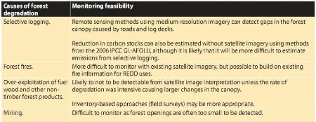
Table 2: causes of degradation and impacts on monitoring (adapted from GOFC-GOLD, 2008)

3. Mapping forest degradation

3.1. Remote sensing in forest degradation

In the idea of the study of Kauppie et al. (2006) the way to quantify change in the forest is to select four forests attributes area, volume, density of growing stock, biomass, and sequester carbon) that provide a useful starting point for global forest monitoring. According to Cogalton (2007), these dates are particularly essential when attempting to estimate forest volume, biomass and carbon using remote sensing technology.

Lambin (1999) explained the role of remote sensing in forest degradation, in this study, the author is trying to explain how spectral, spatial and temporal information could be used to access the concept of forest degradation.

In the study of Herold et al. (2009) they explained that mapping forest degradation with remote sensing data is more challenging than mapping deforestation because the degraded forest is a complex mix of different land cover types (vegetation, dead trees, soil, shade) and the spectral signature of the degradation changes quickly (i.e., < 2 years) (Souza et al. 2009 in herold et al). High spatial resolution sensors such as Landsat, ASTER and SPOT have been mostly used so far to address forest degradation. However, very high resolution satellite imagery, such as Ikonos or Quickbird, and aerial digital imagery acquired with videography has been used as well. Methods for mapping forest degradation range from simple image interpretation to highly sophisticated automated algorithms (GOFC-GOLD,2008).

Higher spatial resolution imagery is more suitable for detection of specific forest degradation impacts. For example, Ikonos imagery can easily detect forest canopy structural damage (Read et al., 2003; Souza, Jr et al., 2005), but, given the cost for image acquisition and computational challenges to extract information from these very high spatial resolution images, their use in operational applications such as monitoring logging is limited.

3.2. Forest change detection analysis

Various classifications of change in forest ecosystems have been proposed. Aldrich (1985) approached the variability in forest cover from a thematic angle, enumerating nine general forest disturbance classes: no disturbance, harvesting (areas subjected to timber removal operations), silvicultural treatments (e.g., thinning), land clearing (vegetation removal and site preparation), insect and disease damage (epidemic conditions), fire (prescribed burning and wildfire), flooding (man-caused and natural), regeneration (artificial or natural), Other (not fitting any of the above categories).

Coppin (2001) tried to explain different types of change detection in forest ecosystems with remote sensing using digital imagery, he used many techniques change detection, image acquisition, data reprocessing for change detection methods, multidimensional temporal feature space analysis, image differencing, etc.

Since early days of earth observation systems, various techniques of change detection have been developed for forest monitoring using high resolution optical remote sensing. These approaches are focused on the identification of forest cover change, described by Geist (2006),

Highly Detectable		Detection limited & increasing data/effort		Detection very limited
·	Deforestation	·	Selective logging	·	Harvesting of most non-
·	Forest fragmentation	·	Forest surface fires		timber plants products
·	Recent slash-and-burn	·	A range of edge-effects	·	Old-mechanized
	agriculture	·	Old-slash-and-burn		selective logging
·	Major canopy fires		agriculture	·	Narrow sub-canopy
·	Major roads	·	Small scale mining		roads (<6m wide)
·	Conversion to tree monocultures	·	Unpaved secondary roads (6-20m wide)	·	Understorey thinning and clear cutting
·	Hydroelectric dams and other forms of flood disturbances	·	Selective thinning of canopy trees	·	Invasion of exotic species
·	Large-scale mining

Table 3: Forest degradation activities and their degree of detection using Landsat-type data, Source:

The literature indicates that forest canopy changes can be detected by a variety of analysis methods. Although most methods provide generally positive results, few studies have compared and evaluated alternative approaches. Since Singh's 1999 paper, two recent studies have attempted to determine what change detection method is most appropriate.

Using SPOT multispectral, multitemporal data, Muchoney and Haack (2004) compared four methods, merged PCA, image differencing, spectral temporal change classification, and post-classification change differencing, for identifying changes in hardwood defoliation by gypsy moth. Defoliation was most accurately detected by the image differencing and PCA approaches.

Collins and Woodcock (1996) have compared three linear change detection techniques, multitemporal Kauth-Thomas, PCA, and Gramm-Schmidt orthogonalization. Better and similar results were obtained with the multitemporal Kauth-Thomas and PCA methods than for the Gramm-Schmidt technique; however, the authors recommended the Kauth-Thomas approach because it identifies change in a more consistent and interpretable manner. These authors also examined to what extent the digital images should be preprocessed.

3.3. Direct methods of mapping forest degradation

Visual interpretation of high resolution data can detect canopy damage in some cases (Saatchi et al., 2007). Spatial patterns of log landings (patios for logging trucks and river landings) and identification of other infrastructure (e.g. roads and rivers used for transportation) has been a successful approach for identifying degradation (Asner et al., 2005). Likewise deforestation and forest degradation can be mapped with different techniques, varying from visual interpretation to advanced image processing algorithms.

Among the most classically used techniques Herald et al.,2009; related some of them Visual interpretation, which can easily detect canopy damage areas in very high spatial resolution imagery; ii) automate segmentation; iii) spectral mixing analysis for logging disturbances (Asner et al. 2005, Oliveira et al. 2007) and fire (Souza et al. 2005); iv) lacunarity indices for canopy structural characterization (Malhi and Román-Cuesta 2008); vi) Hyperspectral automated canopy identification (Palace et al. 2008).

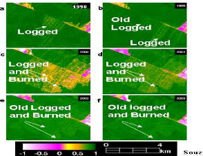
Figure 5: Spectral mixing analysis (SMA) as a way to follow the degradation dynamics of Amazonian
lowland forests using Ikonos sensors (Souza et al. 2005),

For example Asner et al. (2005) developed automated algorithms to identify logging activity with Landsat data. Detection of active fires with thermal data can also indicate presence of subsequent burn scars (Roy et al., 2005).An effective solution for identifying degraded forests from proximity to infrastructure has recently been proposed to take advantage of existing observational approaches given the current limitation in knowledge on the spatial distribution of biomass (Mollicone et al., 2007).

3.4. Indirect methods of forest degradation mapping

In the study of herald et al. (2009), they tried to explain in detail this method as The indirect method is useful when degradation intensity is low and the area to assess is large, when satellite imagery is not easily accessible, or when the direct approach cannot be applied for whatever other reason. An example of a useful indirect approach is the «intact forest» approach where the spatial distribution of human infrastructures (i.e. roads, population centres) are used as proxies, so that the absence of these are used to identify forest land without anthropogenic disturbance

(intact forests) so as to assess the carbon content present in the disturbed and non-disturbed forest lands (Mollicone et al. 2007; Potopov et al. 2008 in Herald et al, 2009):

According to this previeous study of herald, Scenario modelling for forest degradation would be another indirect method which could be applied to estimate both future and historical forest degradation dynamics..

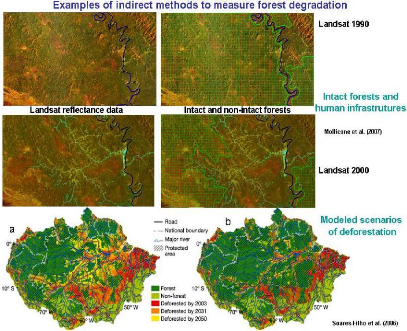
Figure 6: Estimation of intact and non-intact forests based on areas of influence (buffers) from human infrastructures Soares-Filho et al. 2006

3.5. Relevancy of different forest degradation approach

In the study of Achanya and Dangi, 2009 they tried to develop a relevancy of different forest degradation assessment in Nepal. This method can also be applied in the tropical region of Africa.

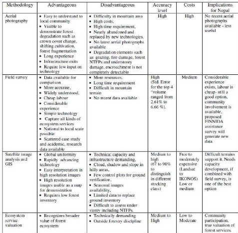
Table 3 : Relevance of different forest degradation approach, source: Acharya and Dangi, 2009

3.6. The use of vegetation indices as NDVI concept to assess forest degradation

Vegetation indices are the quantitative measure of measuring biomass or vegetation vigour, usually formed by a combination of several spectral bands; whose values are added, divided or multiplied in order to yield a single value that indicates the amount or vigour of vegetation. A variety of vegetation indices have been developed, with most commonly using red and near infrared regions of the spectrum to emphasize the difference between strong absorption of red

electromagnetic radiation and the strong scatter of near infrared radiation. The simplest form of vegetation index is a ratio between near infrared and red reflectance and it is high for healthy living vegetation. Literature survey revealed wide disagreement regarding the biomass and vegetation indices relationship. Many studies report a significant positive relationship ( Boyad et al., 1999 ) while some results showed poor relationship ( Foody et al.,2003,schlerf et al.,2005).

The normalized difference index is one of the most commonly used vegetation indices in many applications relevant to analysis of biophysical parameter of forests. Over past two decades its utility has been well demonstrated in satellite assessment and monitoring of global vegetation cover (Huete and Liu,1994,leprieur et al 2000). The strength of NDVI is in its rationing concept which reduces many form of multiplicative noise present in multiple bands. However, conclusions about its value vary depending on the use of specific biophysical parameters and characteristics of the study area. (Deo, 2008).It is computed by the product of the ratio of two electro-magnetic wavelengths (near infrared- red )/(near infrared+red). Vegetation has a high near chlorophyll pigments and the value of NDVI tends to one. In contrast of this, clouds, water, snow etc. have a high red reflectance than near-infrared and these features yield negatives NDVI value. Rocks and bare soil also have similar reflectance and usually zero value of NDVI;

The saturation of the relationship between biomass and NDVI is also a well known problem. This can be explained by the fact that as canopy increases, the amount of red light that can be absorbed by leaves reaches a peak while near-infrared (NIR) reflectance increases because of multiples scattering with leaves. The imbalance between a slight decrease in the red and high NIR reflectance results in a slight change in the NDVI ratio and thus, yield poor relationship with biomass (Tenkabail et al., 2000). Further, Rauste (2005) observed that saturation level is also dependent on the tree species, forest types as well as the ground surface types. Therefore, a suitable relationship of vegetation indices and biomass is crucial in assessment of biomass in different circumstances and a matter of more research work. The usefulness of remote sensing in such work depends on the strength of the relationships developed with respect to a particular type of forests and its geographical location.

3.7. Forest canopy change and remote sensing

Researchers have found relationships between vegetation properties and remotely sensed variables. In order to summarize these diverse experiments, basal area and canopy cover, and the volume and productivity variable includes age, height, volume, diameter and density. Brockhaus et al., (1992) found a significant relationship between green TM band (2) with basal area of trees.

More recent work by Fiorella et al. (2003) found that ratios of near-infrared/red and near-infrared/middle-infrared correlated with structural forms. Cook et al (1989) discovered that vegetation productivity is more strongly related to band ratios than individual bands.

Both the volume and the aboveground biomass (AGB) of forests can be estimated from allometri c relationships with canopy width, structure, and/or height, the intensity of SAR backscatter, corr

Nelson et al (1984) analyzed (simulated) TM data, and concluded most information about vegetation was contained in the blue, near-infrared and middle-infrared. Thermal infrared was used by Holbo and Luvall (1989) to map broad forest type classes. Vegetation dieback and damage are best mapped by band ratios.

3.8. Comparing Forest Inventory and Remote Sensing Measurement for forest degradation mapping

The same forest quantities (e.g., biomass) are estimated differently by ground forest inventory and by remote sensing . Forest inventory typically measures tree abundance, diameter, crown width, species, and height (Song 2007; Chave et al. 2005).

Table 5. How Forest Inventory and Remote Sensing Estimate the Forest Identity, adapted from Fragn et al,2009.

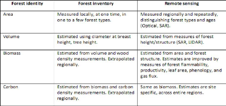
Remote sensing measures reflected spectra, forest area and the horizontal and vertical structure of forests can be measured directly from these reflected spectra. Fieldwork or higher resolution imagery can be used to generate ground-truth data to assess the accuracy of these forest area and structure measurements (Jensen 2007).

3.9. Estimating Forest Volume Using Remote Sensing

elations with passive spectra, and various fusions of the above (Lu et al. 2006; Balzter et al. 2007; Rosenqvist et al. 2003).

3.10. Estimating forest biomass using remote sensing

Biomass cannot be directly measured from remote sensing data, however remotely sensed reflectance can be related to the biomass estimates based on in situ measurements (Dong et al. 2003). Reflections of the red, green and near infrared radiances contained considerable information about forest biomass. Two main approaches predicting biomass using satellite images are (1) Use of Solar radiation and (2) Use of Reflection Coefficients (Namayanga 2002), which is primarily determined by the green foliage biomass (Christensen and Goudriaan, 1993).

Forest height can be measured from a variety of remotely sensed data and used to estimate biomass (Kellndorfer et al. 2004; Palace et al. 2008, Pflugmacher et al. 2008). Although diamete, height, and wood density are central variables, biomass estimates can be improved by using addit ional forest structure variables (e.g., canopy width, canopy volume) (Dubayah et al. 2000; Palace et al. 2008; Popescu et al. 2003).

Direct biomass estimation may also be possible with vegetation Light Detection and Ranging (LIDAR) observations (Popescu 2007; Drake et. al 2002). The potential of forest biomass mapping has also been explored using Radar (Gaveau et al., 2003; Tomppo et al. 2002) along with JAXA ALOS-PALSAR L-band (24 cm wavelength) which gives lower range of biomass (upto 50-80 t/ha). The BIOMASS mission, which is expected to launch around 2014 by ESA uses a longer wavelength (68 cm) and shows potential of estimating higher levels of biomass (FAO,2008).

3.11. Estimating Forest Carbon Stocks from Remotely Sensed Data

Satellite imaging can tell us much about global carbon stocks, but there are limits to its accuracy. Dry biomass is approximately 47.to.55 percent carbon by weight (IPCC 2006), so aboveground b iomass estimates from remote sensing can be simply converted into aboveground carbon (AGC) stock estimates (Gibbs et al. 2007).

Carbon emissions from deforestation and degradation depend not only on the area of forest change but also on the associated biomass loss (Brown, 2002). The IPCC (Penman et al., 2003a) compiled methods and good practice guidance for determining changes in carbon stocks in association with national inventories of greenhouse gas (GHG) emissions (Chapter 3 in Penman et al., 2003a) for changes in Land Use, Land Use Change, and Forestry (LULUCF) and with carbon sequestration projects (Penman et al., 2003a) in the first commitment period. With the updated version of the IPCC guidelines for conducting national GHG emissions from the

LULUCF sector (Penman et al., 2003a; IPCC, 2006), methods are available for estimating GHG emissions from deforestation at the national and project scales.

4. Conclusion

As conclusion of this literature review, we can see that a lot f conclusion can be formulated from this literature review.

Our literature review had three important parts, the first one helped us to understand the concept of remote sensing, the second one was a brief explanation of the concept of forest degradation and the last one explained different methodologies to evaluate the problem of degradation using remote sensing

As a change in forest structure it is not easy to detect the problem through remote sensing, the choice of different approaches depends on a number of factors including the type of degradation process, available (historical) data, capacities and resources and the potentials and limitations of various measurement and monitoring approaches.

Mapping forest degradation should not be only a problem of scientist but a social problem putting together interdisciplinary stakeholders, they must have information of the problem in order to quantify the extent of the threat. the preceding discussion the point 3 of this literature review has explored how advancements in remote sensing techniques would help to gather information and to answering most of these questions about all sides of the definition of forest degradation

The big challenge is now how those methodologies especially in developing country because of the availability of the satellites imagery, increase in new processing technologies methods, and the cost of spatial information.

5. References

Acharya, K., and Dangi, R. 2009. Forest Degradation in Nepal: Review of Data and Methods. FAO Forest Resources Assessment Programme, Rome, Italy

Anderson, J.E., L.C. Plourde, M.E. Martin, B.H. Braswell, M.L. Smith, R.O. Dubayah, M.A. Hof ton, and J.B. Blair. 2008. Integrating waveform lidar with hyperspectral imagery for inve ntory of a northern temperate forest. Remote Sensing of the Environment 112(4): 1856- 1870.

Andersson, K., T.P. Evans, and K.R. Richards. 2009. National forest carbon inventories: Policy needs and assessment capacity. Climatic Change 93(1-2): 69-101.

Askne, J., M. Santoro, G. Smith, and J.E.S. Fransson. 2003. Multitemporal repeat-pass SAR inter ferometry of boreal forests. IEEE Transactions on Geoscience and Remote Sensing 41(7): 1540-1550.

Asner, G. P., M. Keller, R. Pereira, and J. C. Zweede. 2002. Remote sensing of selective logging in Amazonia: Assessing limitations based on detailed field observations, Landsat ETM+, and textural analysis. Remote Sensing of Environment 80:483-496.

Asner, G. P., M. Keller, R. Pereira, J. C. Zweede, and J. N. M. Silva. 2004. Canopy damage and recovery after selective logging in Amazonia: Field and satellite studies. Ecological Applications 14:S280-S298.

Asner, G. P., D. E. Knapp, E. N. Broadbent, P. J. C. Oliveira, M. Keller, and J. N. M. Silva. 2005. Selective logging in the Brazilian Amazon. Science 310:480-482.

Asner, G., Rudel, T., Aide, M., Defries, R., Emerson, R. 2009. A contemporary assessment of change in humid tropical forests. Conservation Biology 23:1386-1395.

Baccini, A., N. Laporte, S.J. Goetz, M. Sun, and H. Dong. 2008. A first map of tropical Africa's aboveground biomass derived from satellite imagery. Environmental Research Letters 3: 1-9

Bicheron, P., P. Defourny, C. Brockmann, L. Schouten, C. Vancutsem, M. Huc, S. Bontemps, Leroy, F. Achard, M. Herold, F. Ranera, and O. Arino. 2008. GLOBCOVER Products Description and Validation Report. MEDIAS-France, ftp://uranus.esrin.esa.int/pub/globc over v2/global/.

DeFries, R. 2008. Terrestrial vegetation in the coupled human-earth system: Contributions of re mote sensing. Annual Review of Environment and Resources 33: 369-390.

Blaschke, T., Lang, S., and G. Hay (Eds.), 2008, Object-Based Image Analysis, Berlin, Germany: Springer-Verlag, 817 p

Brockhaus, J A and S Khorram. 1992. A comparison of Spot andLandsat-TM data for use in conducting inventories of forest resources. IJRS 13, 16, pp 3035-3043.

Campbell, J., 2007, Introduction to Remote Sensing, 4th ed., New York, NY: Guilford Press, 626p.Change Biology 11(6): 945-958.

Chave, J., C. Andalo, S. Brown, M.A. Cairns, J.Q. Chambers, D. Eamus, H. Folster, et al. 2005.

Comparison of various remote sensing data sources in the retrieval of forest stand

Congalton, R. and K. Green, 2009, Assessing the Accuracy of Remotely Sensed Data: Principles and Practices, 2nd ed., Boca Raton, FL: CRC/Taylor & Francis, 183 p.

Congalton, R., 2010, «How to Assess the Accuracy of Maps Generated from Remotely Sensed Data,» in Manual of Geospatial Science and Technology, 2nd ed., Bossler, J. (Ed.), Boca Raton, FL: Taylor & Francis, 403-421.

Cook E A, L R Iverson and R L Graham. 1989. Estimating forest productivity with Thematic Mapper and biogeographical data.Remote Sens of Environ 28, pp 131-141.

Cramer, W., A. Bondeau, S. Schaphoff, W. Lucht, B Smith and S. Sitch 2004. Tropical forests and the global carbon cycle: impacts of atmospheric carbon dioxide, climate change and rate of deforestation. Phil. Trans. Roy. Soc. Lond. B 359: 331-343.

Danson, F M and P J Curran. 1993. Factors affecting the remotely sensed response of coniferous forest plantations. Remote Sensing of Environ 43, pp 55-65.

De Wulf, R R, R E Goosens, B P De Roover and F C Borry. 1990.Extraction of forest stand parameters from panchromatic and multi-spectral Spot-1 data. IJRS 11, 9, pp 1571-1588.

DeFries, R., F. Achard, S. Brown, M. Herold, D. Murdiyarso, B. Schlamadinger, and C. de Souz a. 2007. Earth observations for estimating greenhouse gas emissions from deforestation in developing countries. Environmental Science and Policy 10(4): 385-394.

GOFC-GOLD. 2009. A sourcebook of methods and procedures for monitoring and reporting anthropogenic greenhouse gas emissions and removals caused by deforestation, gains and

Donnellan, A., P. Rosen, J. Graf, A. Loverro, A. Freeman, R. Treuhaft, R. Oberto, et al. 2008. Deformation, ecosystem structure, and dynamics of ice (DESDynI). Paper presented at th e ESRI International User Conference. April 2008, Washington, DC.

FAO. 2002. Food and Agriculture Organization. Proceedings: Second Expert Meeting on Harmonizing Forest-related Definitions for Use by Various Stakeholders. Rome, 11-13 September 2002. Rome. http://www.fao.org/docrep/005/y4171e/y4171e00.htm

FAO. 2006a. Food and Agriculture Organization .Global Forest Resources Assessment

Fiorella, M and W J Ripple. 1993. Determining successional stage of temperate coniferous forests with Landsat satellite data. PE&RS59, 2, pp 239-246.

Foody, G.M. 2002. Status of land cover classification accuracy assessment. Remote Sensing of Environment 80(1): 185-201

Franklin J F, F W Davis and P Lefebvre. 1991. Thematic Mapper analaysis of tree cover in semiarid woodlands using a model of canopy shadowing. Remote Sens of Environ 36, pp 189-202.

Foody,G.M.,Boyad,D.S.,Cutler M.E.J.,2003.Predictive relations of tropical forest biomass from landsat TM data and their transferability between regions.Remote Sensing of environment 84(4):463-474.

Gao, X., A.R. Huete, W.G. Ni, and T. Miura. 2000. Optical-biophysical relationships of vegetation spectra without background contamination. Remote Sensing of Environment 7 4(3): 609-620

Gibbs, H.K., S. Brown, J.O. Niles, and J.A. Foley. 2007. Monitoring and estimating tropical

forest carbon stocks: Making REDD a reality. Environmental Research Letters 2(4): 045023.

Jensen, J., 2005, Introductory Digital Image Processing: A Remote Sensing Perspective, 3rd ed., Upper Saddle River, NJ: Pearson Prentice Hall, 526 p.

losses of carbon stocks in forest remaining forests, and forestation. GOFC-GOLD Report version COP15-1.Available at www.gofc-gold.uni-jena.de/redd/.

Hame, T, E Tomppo and E Parmes. 1988. Stand based forest inventory from Spot Image. Symp proc: Spot-1, Image Utilisation,Assessment, Results. CNES, Cepadues Editions, Toulouse, France,pp 971-976.

Herold, M., Yasumasa H., Patrick V.,Asner G., Victoria Heymell⁵, Rosa María Román-Cuesta⁶

Houghton, R.A. 2005. Aboveground forest biomass and the global carbon balance. Global Change Biology 11(6): 945-958

Huete, A. R., Miura, T., & Gao, X. (2003). Land cover conversion and degradation analyses

through coupled soil-plant biophysical parameters derived from hyperspectral EO-1 Hyperion. IEEE Transactions on Geoscience and Remote Sensing, 41(6), 1268-1276.

Hyyppa, J., H. Hyyppa, M. Inkinen, M. Engdahl, S. Linko, and Y.H. Zhu. 2000. Accuracy comparison of various remote sensing data sources in the retrieval of forest stand attributes . Forest Ecology and Management 128(1-2): 109-120.

Hyyppa, J., H. Hyyppa, D. Leckie, F. Gougeon, X. Yu, and M. Maltamo. 2008. Review of methods of small-footprint airborne laser scanning for extracting forest inventory data in b oreal forests. International Journal of Remote Sensing 29(5): 1339-1366

IPCC. Intergovernmental Panel on Climate Change. 2003. Good Practice Guidance on Land Use, Land-Use Change and Forestry. Eggleston, H.S.,Buendia, L., Miwa, K., Ngara, T. and Tanabe, K. (eds.). National Greenhouse Gas Inventories Programme. Institute for Global

ITTO. 2005. International Tropical Timber Organization. 2005. Status of tropical forest

Jensen, J. R., Im, J., Jensen, R., and P. Hardin, 2009, «Image Classification,» in Handbook of Remote Sensing, Nellis, D. and T. Warner (Eds.), Boca Raton, FL: CRC Press, 82-102 (Chapter 19).

Jensen, J., 2007, Remote Sensing of Environment: An Earth Resource Perspective, 2nd ed., Upper Saddle River, NJ: Pearson Prentice Hall, 592 p.

Kauppi, P.E., J.H. Ausubel, J.Y. Fang, A.S. Mather, R.A. Sedjo, and P.E. Waggoner. 2006. Returning forests analyzed with the forest identity. Proceedings of the National Academy of Sciences of the United States 103(46): 17574-17579.

Kayitakire, F., C. Hamel, and P. Defourny. 2006. Retrieving forest structure variables based on image texture analysis and IKONOS-2 imagery. Remote Sensing of Environment 102(3- 4): 390-401.

Kellndorfer, J., W. Walker, D. Nepstad, C. Stickler, P. Brando, P. Lefebvre, A. Rosenqvist, and M. Shimada. 2008. Implementing REDD: The potential of ALOS/PALSAR for forest mapping and monitoring. Paper presented at the Second GEOSS Asia-Pacific

Kimes, D.S., K.J. Ranson, G. Sun, and J.B. Blair. 2006. Predicting lidar measured forest

vertical structure from multi-angle spectral data. Remote Sensing of Environment 100(4): 503-511.

Leprieur,P.E. ;Kerr ?Y.H.,Mastorchio,S.,Meunier,J .C.,2000 .Monitoring vegetation cover across semi-arid regions:comparision of remote observations from various scales.International journal of remote sensing21:281-300.

Lu, D.S. 2006. The potential and challenge of remote sensing-based biomass estimation. International Journal of Remote Sensing 27(7): 1,297-1,328

Luus, K.A., and R.E.J. Kelly. 2008. Assessing productivity of vegetation in the Amazon using M. Shimada. 2008. Implementing REDD: The potential of ALOS/PALSAR for forest

Malhi, Y., J.T. Roberts, R.A. Betts, T.J. Killeen, W.H. Li and C.A. Nobre. 2008. Climate change, deforestation, and the fate of the Amazon. Science 319: 169-172.

Maltamo, M., K. Eerikainen, P. Packalen, and J. Hyyppa. 2006. Estimation of stem volume mapping and monitoring. Paper presented at the Second GEOSS Asia-Pacific Marrakech Accords. Bonn, Germany.

Means, J.E., S.A. Acker, D.J. Harding, J.B. Blair, M.A. Lefsky, W.B. Cohen, M.E. Harmon, and
methods of small-footprint airborne laser scanning for extracting forest inventory

Mollicone D., Achard F., Federici S., Eva H.D., Grassi G., Belward A., Raes F., Seufert G., Stibig H.-J., Matteucci G., Schulze E.-D. 2007. An incentive mechanism for reducing emissions from conversion of intact and non-intact forests. Climatic Change 83: 477- 493.

Nelson, R F, R S Latty and G Mott. 1984. Classifying northern forests using thematic mapper simulator data. PE&RS 50, 5, pp 607-617.

Nemani, R, P S Running and L Band. 1993. Forest ecosystem processes at the watershed scale: sensitivity to remotely-sensed LeafArea Index estimates. IJRS 14, 13, pp 2519-2534.

Oliveira, P. J. C., G. P. Asner, D. E. Knapp, A. Almeyda, R. Galvan-Gildemeister, S. Keene, R. Raybin, and R. C. Smith. 2007. Land-use allocation protects the Peruvian Amazon. Science 317:1233-1236.

Page, S.E., F. Siegert, J.O. Rieley, H.D.V. Boehm, A. Jaya, and S. Limin. 2002. The amount of c arbon released from peat and forest fires in Indonesia during 1997. Nature 420(6911): 61 -65.

Palace, M., Keller, M., Asner, G., Hagen, S., and B. Braswel. 2008. Amazon Forest Structure from IKONOS Satellite Data and the Automated Characterization of Forest Canopy Properties. Biotropica 40: 141-150

Patenaude, G., R. Milne, and T.P. Dawson. 2005. Synthesis of remote sensing approaches for

forest carbon estimation: Reporting to the Kyoto Protocol. Environmental Science and Policy 8(2): 161-178.

Peres, C., Barlow, J., and Laurance, W. 2006. Detecting anthropogenic disturbance in tropical forests. TRENDS in Ecology and Evolution 21, 227-229.

Peterson, L.K., K.M. Bergen, D.G. Brown, L. Vashchuk, and Y. Blam. 2009. Forested land-cover patterns and trends over changing forest management eras in the Siberian Baikal region. Forest Ecology and Management 257(3): 911-922

Popescu, S.C., R.H. Wynne, and R.F. Nelson. 2003. Measuring individual tree crown diameter with lidar and assessing its influence on estimating forest volume and biomass. Canadian Journal of Remote Sensing 29(5): 564-577.

Rosenqvist, A., A. Milne, R. Lucas, M. Imhoff, and C. Dobson. 2003. A review of remote sensing technology in support of the Kyoto Protocol. Environmental Science and Policy 6(5): 441-455

Simula, M. 2009. Towards defining forest degradation: comparative analysis of existing definitions. Forest Resources Assessment. Pp 57. Working Paper 154. FAO, Rome. ftp://ftp.fao.org/docrep/fao/012/k6217e/k6217e00.pdf

Smith, J A, T L Lin et al. 1980. The Lambertian assumption andLandsat data. PE&RS 46, 9, pp 1183-1189.

Song, C. 2007. Estimating tree crown size with spatial information of high resolution optical remotely sensed imagery. International Journal of Remote Sensing 28(15): 3305- 3322

Song, C., T.A. Schroeder, and W.B. Cohen. 2007. Predicting temperate conifer forest successional stage distributions with multitemporal Landsat Thematic Mapper imagery. Remote Sensing of Environment 106(2): 228-237

Souza, C., L. Firestone, L. M. Silva, and D. Roberts. 2003. Mapping forest degradation in the Eastern Amazon from SPOT 4 through spectral mixture models. Remote Sensing of Environment 87:494-506.

Souza, C., D. A. Roberts, and M. A. Cochrane. 2005. Combining spectral and spatial information to map canopy damages from selective logging and forest fires. Remote Sensing of Environment 98:329-343.

Souza, C., Cochrane, M., Sales, M., Monteiro, A., Mollicone, D. 2009. Integrating forest transects and remote sensing data to quantify carbon loss due to forest degradation in the Brazilian Amazon, FRA Working Paper 161

Tucker, C J. 1979. Red and photographic infrared linear combinations for monitoring vegetation. Rem Sens of Environ 8, pp 127-150.

Tucker, C.J., J.R. Townshend, and T.E. Goff. 1985. African land-cover classification using satellite data. Science 227: 369-375.

UNFCCC (United Nations Framework Convention on Climate Change). 2001. COP-7: The Marrakech Accords. Bonn, Germany.

Forest degradation, a methodological approach usingremote sensing techniques: literature review

Table of contents