A GIS-BASED
MODELING OF ENVIRONMENTAL HEALTH RISKS
IN POPULATED AREAS OF PORT-AU-PRINCE, HAITI
By
Myrtho Joseph
________________________________
A Thesis submitted to the Faculty of the
SCHOOL OF NATURAL RESSOURCES
In Partial Fulfillment of the Requirements
For the Degree of
MASTER OF SCIENCE
WITH A MAJOR IN RENEWABLE NATURAL RESOURCES STUDIES
In the Graduate College
THE UNIVERSITY OF ARIZONA
2007
STATEMENT BY AUTHOR
This thesis has been submitted in partial fulfillment of
requirements for an advanced degree at The University of Arizona and is
deposited in the University Library to be made available to borrowers under
rules of the Library.
Brief quotations from this thesis are allowable without special
permission, provided that accurate acknowledgment of source is made. Requests
for permission for extended quotation from or reproduction of this manuscript
in whole or in part may be granted by the head of the major department or the
Dean of the Graduate College when in his or her judgment the proposed use of
the material is in the interests of scholarship. In all other instances,
however, permission must be obtained from the author.
SIGNED: ____________________________
APPROVAL BY THESIS COMMITTEE
This thesis has been approved on the date shown below:
_____________________________ ________________
D. Phillip Guertin Date
Associate Professor of Watershed Management
_____________________________ ____________________
Craig Wissler Date
Assistant Professor Landscape Studies
_____________________________ ____________________
Gary Christopherson Date
Director, Center for Applied Spatial Analysis
ACKNOWLEDGEMENTS
Without any doubt the success of a study like this relies on a
well-thought methodology, an excellent design, a good theoretical background,
reliable data and tools, and a sound analysis. However, without the support of
people who are expert in specific domains, this study would be
more challenging and might not be made possible. A popular and wise biblical
verse says: «People die for lacking knowledge». I would not
physically die without access to some precious information released by many of
those who helped, but I would be dying slowly with impatience, discouragement,
sense of defeat, lack of inspiration, and frustration.
I want to take advantage of this occasion to thanks D. Phil
Guertin who has been my advisor not only for the thesis but during the complete
course of my studies at the School of Natural Resources. His support has gone
beyond academics, and covered a large range of assistance that is not possible
to list without missing some. I am more than certain Dr Guertin will continue
to guide me even after the completion of my master's study. I want to express
my gratitude to Dr Christopherson who opened the CASA Lab for me during the
tedious digitization process and had provided me profitable guidance for the
generation of Port-au-Prince's DEM. My appreciation goes to Wissler for
sporadic but precious intervention when I was struggling with some ArcMap
processes. Mickey Reed was irreplaceable for specific advice and access to
fine-point tools and processes. Thanks to all the Advanced Resource
Technology's staff for unconditional support and flexibility. I am grateful to
Kareen Thermil, who granted me access to some precious information and data,
and Juvenel Joseph, my brother who did any necessary arrangement to facilitate
acquisition of much of the data needed and available from Haiti. I want to
thank either the group of Haitian professionals and students who accepted to
participate in the EOW survey. Finally, the best for last, I want to thank my
wife who accepted heartedly to sacrifice our time and invest it in the
accomplishment of the thesis. Her devotion and support were priceless for the
completion of my study.
DEDICATION
This thesis is dedicated to my mother who would not have the
opportunity to witness the fulfillment of my dream; to my wife whose
unconditional support helped me to be at the same time a father, a spouse, and
a fulltime master's student; finally to my country which unfortunately is the
inspiration of this topic.
TABLE OF CONTENTS
LIST OF TABLES
8
LIST OF FIGURES
9
ABSTRACT
13
1. INTRODUCTION
15
2. LITERATURE
REVIEW
18
2.1 RISK
18
2.2 HAZARDS
19
2.3
VULNERABILITY
19
2.4 RISK
ASSESSMENT
20
2.5 HAZARD
IDENTIFICATION OR DELINEATION
22
2.6 ENVIRONMENTAL
HEALTH FACTORS
23
2.7 APPROACHES TO
VULNERABILITY ASSESSMENT
25
2.8 MULTI-CRITERIA
EVALUATION (MCE) AND WEIGHTED LINEAR COMBINATION (WLC)
28
2.9 CLASSIFICATION
METHODS
30
3. METHODS
31
3.1 STUDY AREA
31
3.2 DATA
COLLECTION
33
3.3 DATA
LIMITATION
34
3.4 CONSTRUCTION OF
THE MODEL
35
3.4.1 Process Overview
35
3.4.2 Environmental Health
Factors
36
3.4.2.1 Air pollution from
traffic
36
3.4.2.2 Waste Pollution
39
3.4.2.3 Public formal and
informal market places
42
3.4.2.4 Hospitals and the main
cemetery
43
3.4.2.5 Housing density
44
3.4.2.6 Pollution from water
bodies
47
3.4.2.7 Proximity to the
sea
48
3.4.2.8 Proximity to high
voltage power line
49
3.4.3 Linear Combination of the
Variables
50
3.4.4 Classification
Schemes
51
3.5 MODEL'S
SUMMARY
52
4. RESULTS AND
DISCUSSION
53
4.1 RESULTS BY
LINEAR COMBINATION SCHEMES
54
4.1.1 Expert Opinion Survey,
Equal Influence (Equal Weight), and Personalized Weightings
54
4.1.2 The Maximum Weighting
Scheme
57
4.2
COMPARISON OF THE CLASSIFICATION TECHNIQUES
59
4.3
NEIGHBORHOODS EXPOSED AT HIGH RISKS
61
4.4 ENVIRONMENTAL
HEALTH HAZARDS
63
4.4.1 Traffic Pollution
65
4.4.2 Waste Pollution
66
4.4.3 Housing Density
67
4.4.4 Pollution from Market
Places
68
4.4.5 Pollution water
bodies
69
4.4.6 Pollution from the
coast
71
4.4.7 Pollution from high
voltage electric power
72
4.4.8 Pollution from the
hospitals
73
4.4.9 Pollution from the
cemetery
74
4.5 SENSITIVITY
ANALYSIS
75
4.5.1 Traffic Pollution
Influence
75
4.5.2 Waste Pollution
Influence
76
4.5.3 Proportional Spatial
Incidence of the factors
77
5. CONCLUSIONS
77
APPENDIX A - TABLES
81
APPENDIX B - FIGURES
89
APPENDIX C - MODEL'S OUTLINE
99
APPENDIX D - MODEL'S EXECUTION SCRIPT
100
REFERENCES
117
LIST OF TABLES
Table 1: Pollution from Traffic - Risk
Thresholds
39
Table 2: Pollution from Waste - Risk Levels
42
Table 3: Pollution from Market Places and Risk
Levels
43
Table 4: Housing Density classification in the
original grid
46
Table 5: Housing Density and Risk Levels
47
Table 6: Pollution from water bodies - Risk
Levels
48
Table 7: Distance to the sea and Risk Levels
49
Table 8: Distance to High Voltage Power Lines and
Vulnerability level
50
Table 9: Percent of areas per vulnerability level -
Average score for the four classification techniques
55
Table 10: Percent of areas by risk level and
aggregation scheme using a standardized classification
55
Table 11: Increase in traffic pollution weight
compared to EOW
76
Table 12: Increase in waste pollution weight
compared to EOW
76
Table 13: Comparison of EOW and Proportional
Incidence Weighting Results
77
Table 14: Risk of Air pollution from traffic -
Vulnerability scales
81
Table 15: EOW Results
82
Table 16: Results for different combination and
classification schemes
83
Table 17: Summary results for the classification
schemes
84
Table 18: Summary Results by Health Hazard and Risk
Level
85
Table 19: Weighting schemes and Results Ranking
86
Table 20: Regression of EOW on Percent of High and
Very High Risks
86
Table 21: Regression of Own Weight on Percent of
High and Very High Risks
87
Table 22: Regression of EOW on Average of Area
Covered (%)
87
Table 23: Regression of Own Weighting on Percent of
Area (%)
88
LIST OF
FIGURES
Figure 1: left: Base map of Port-au-Prince and the
study area; right: Port-au-Prince's view from the southeast hills.
33
Figure 2: Housing Density as classified in the
original grid 0.5x0.5 km
46
Figure 3: Housing Density after reclassification
(grid size: 0.3x0.3 km)
46
Figure 4: Environmental Health Risks -
56
Figure 5: Environmental Health Risks in
Port-au-Prince - EOW classified with the geometric interval technique
57
Figure 6: Environmental Health Risks in
Port-au-Prince - Maximum combination technique using the Geometric Interval
classification method
58
Figure 7: Environmental Health Risks in
Port-au-Prince - Percent of area at-risk by classification technique
60
Figure 8: Environmental Health Risks - Own
weighting scheme using the quantile technique: greater proportion of high/very
high risks
61
Figure 9: Environmental Health Risks - Own
weighting scheme using the geometric interval technique: smaller proportion of
high/very high risks
61
Figure 10: Environmental Health Risks in
Port-au-Prince: Percent of areas at-risk using the Own weighting scheme and the
natural breaks classification method
62
Figure 11: Factors affecting environmental health
in Port-au-Prince.
65
Figure 12: Risks of traffic pollution in
Port-au-Prince
66
Figure 13: Waste Pollution in Port-au-Prince
67
Figure 14: Housing Density in Port-au-prince
68
Figure 15: Pollution from market places
69
Figure 16: Pollution from Water bodies
70
Figure 17: Pollution from the sea coast
72
Figure 18: Pollution from high voltage power
73
Figure 19: Neighborhood pollution from
Hospitals
74
Figure 20: Neighborhood pollution from the central
cemetery
75
Figure 21: EOW - Quantile
89
Figure 22: EOW - Natural Breaks
89
Figure 23: EOW - Geometric Interval
classification
90
Figure 24: EOW- Equal Interval
90
Figure 25: EOW - Defined Interval
91
Figure 26: Equal Weight - Quantile
91
Figure 27: Equal Weight - Natural Breaks
92
Figure 28: Equal Weight - Equal Interval
92
Figure 29: Equal Weight - Geometric Interval
93
Figure 30: Equal Weight - Defined Interval
93
Figure 31: Own Weight - Quantile
94
Figure 32: Own Weight - Natural Breaks
94
Figure 33: Own weight - Equal interval
95
Figure 34: Own Weight - Geometric Interval
95
Figure 35: Own weight - Defined
96
Figure 36: Maximum Output using no classification
technique
96
Figure 37: Maximum Weighting - Defined
97
Figure 38: Traffic Sensitivity Analysis
97
Figure 39: Waste Sensitivity Analysis
98
Figure 40: Proportional Weighting Sensitivity
Analysis
98
LIST OF ABBREVIATIONS
AHP: Analytical Hierarchy Process
ARIs: Acute Respiratory Infections
BMRC: Bureau of Meteorology Research Center
CDERA: Caribbean Disaster Emergency Response Agency
DDI: Disaster Deficit Index
DRI: Disaster Risk Index
ECVH: Enquête sur les Conditions de Vie en Haiti
EHR : Environmental Health Risks
EMMUS II: Enquête de Mortalité, Morbidité et
Utilisation de Services 1994
EMMUS III : Enquête de Mortalité,
Morbidité et Utilisation de Services 2000
EOW: Expert Opinion Survey
EPA: Environment Protection Agency
ESRI: Environmental System Research Institute
GDP: Gross Domestic Product
IDB: InterAmerican Development Bank
IDEA: Instituto de Estudios Ambientales
IDW: Inverse Distance Weighting
IHSI: Institut Haitien de Statistiques et d'Informatique
LDI: Local Disaster Index
MCE : Multi-Criteria Evaluation
PAHO : Panamerican Health Organization
SDE: Section D'Enumeration
SEI: Stockholm Environment Institute
SMCRS: Service Metropolitain pour la Collecte des Residus
Solides
UNDP: United Nations Development program
UNDRO: United Nations Disaster Relief Organization
UNEP: United Nations Environment Program
UNISDR: International Strategy for Disaster Reduction
UTSIG/CNIGS: Unite de Teledetection et de Systeme d'Information
Geographique/ Centre National de l`Information Geo-Spatiale
VIP's: Very Important Points
WHO: World Health Organization
WLC: Weighted Linear Combination
YTV: Helsinki Metropolitan Area Council
ABSTRACT
In Port-au-Prince, Haiti's capital, the increasing occurrence and
casualties from landslides and floods during the last few years has focused
interest toward these natural disasters. The high pressure of human
settlements associated with urban migration constitutes the main trigger of
these deadly events by increasing the sensitivity of the environment as well as
people's vulnerability. Long term impacts of environmental degradation on
health related to human settlements have not received as much attention as
natural disasters. The inconspicuous nature of environmental health hazards
and their related consequences may have diverted stakeholders and people's
attention from them. Health hazards derived from the environment are believed
to be of a greater spatial extent, cause more losses than any other hazards,
and concern more than two-third of the population within the study area. The
objective of this study was to identify areas where such health hazards exist
and assess neighborhoods' vulnerability to these hazards using a GIS modeling
approach that offers the capability of superimposing multiple parameters. Nine
factors were combined with different weighting schemes including an Expert
Opinion survey. Moreover, several classification techniques were tested and
compared in the final process of determining the four risk levels. Finally, a
sensitivity analysis was performed to assess the responsiveness of the model to
changes induced in the model's parameters.
Though this study was conducted in a context of poor data
availability, the results suggest that about 41% of the entire area was
subjected to high risk. Pollution originated from water bodies, traffic and
waste were found as the most critical, while housing density, which is
simultaneously a risk and a vulnerability factor represented the main trigger
of many risks encountered. This study called for a deeper investigation of the
state of pollution in Port-au-Prince by taking direct field measurement in
order to validate the findings. In addition, it reveals the needs for a
synergistic effort of governmental and non-governmental institutions to produce
and make available spatial data at fine scale and resolution in a
cost-efficient manner.
1. INTRODUCTION
Throughout the world, natural disasters have occurred over the
last decades with increasing frequency and have resulted in significant
mortality, morbidity, and disability among people affected, causing the
destruction of physical assets and damaging social resources (UNDP 2004). They
also increase the vulnerability of people, communities, and areas impacted by
weakening or disabling local infrastructure, livelihoods, businesses, and
regional economy (UNDP 2004). If on a global scale global warming, climatic
change, and decadal variations are considered as external (but distant
consequences of anthropogenic influences) triggers of the escalating of number
and intensity of natural disasters, at local scale other human-induced factors
such as population growth, unplanned urbanization, alteration of the natural
environment, under-standard dwellings, augmentation of impervious areas, and
land cultivation increases people exposure to hazards (Sorensen et al. 2006,
Smucker et al. 2007). An increasingly larger proportion of the world's
population is being exposed to locations at high risk (Huppert and Sparks
2006). This phenomenon is mostly observed in mega cities. Indeed, the world's
population is being progressively concentrated in urban areas rather than in
rural areas. It is predicted that in 2007, for the first time, more people
will live in urban centers than in the countryside (Huppert and Sparks
2006).
Throughout the last three decades, the intensification of
migration to urban centers, particularly in Port-au-Prince, Haiti, has resulted
in the proliferation of anarchic and precarious habitats, the degradation of
the resources of the environment, the deficiency of urban services, and the
rupture of ecological equilibrium (IHSI 2003). Water supply and basic
sanitation services are still very deficient. The 1998 edition «Health in
the Americas» report of PAHO/WHO (1998) describes the situation in
Port-au-Prince as follows:
«Solid waste management is a serious problem; bad
excreta disposal practices are polluting almost all 18 water sources supplying
Port-au-Prince. Drainage systems are inadequate and any major storm produces
serious flooding. The growing number of motor vehicles and their inadequate
maintenance have created a serious air pollution problem in
Port-au-Prince.»
Some illustrations of the effect of environmental degradation on
health are the high infestation of dengue in urban areas and the outbreak
reported in 1994 in Port-au-Prince (PAHO 2001); acute respiratory infections
(ARIs) accounted for 25% of deaths among children under 5 years of age, and
suffered by 20% of children of this age group (EMMUS II 1994); and
cardiovascular diseases that caused of the admission of 40% of patients at the
State University Hospital in 1996 (PAHO 2001).
The United Nations Development Program (UNDP) (1994) considers an
event a disaster when the number of human deaths is greater than 10. However,
casualties resulting from environmental health hazards can be easily overlooked
or even disregarded because, unlike floods or landslides that are spatially and
temporally punctual, and with evident physical materialization, environmental
health effects are discreet and continuous over space and time. Often the
effects are not actually associated with their causes yet the casualties are
countless and exceed victims of natural disasters.
On one hand it is recognized that a healthier physical
environment is among the factors associated with a decline in morbidity and
mortality in the past century (Corvalan et al. 1999). On the other hand high
population density is considered one of the vectors responsible for health
degradation and aggravation in poor countries (Campbell-Lendrum and Corvalan
2007). According to some estimates, one third of the global urban population
and over 70% of people in urban developing countries live in slum-like
conditions characterized by poor housing and meager basic services, with
ineffective regulation of pollution (Campbell-Lendrum and Corvalan 2007).
However, the impact of population densification on living conditions and
health is not sufficiently well perceived, at least at the community spatial
level. While qualitative information depicts the severe conditions in which
the population is living, it is difficult, if not impossible, to find detailed
quantitative data about the spatial incidence of a specific health hazard in
Port-au-Prince. The spatial study unit used in surveys on living conditions is
very coarse and doesn't allow acknowledging the reality at finer spatial scale.
In Port-au-Prince, in addition to the intense degradation of the environment
aforementioned, the average density found from the SDE1(*) is more than 61,300 inhabitants
per km2. In some places, the density caps to more than one million
per km2. There's a proliferation of diseases among the population
particularly in neighborhoods exposed to degraded environmental conditions such
as water stagnation, waste accumulation, poorly cleaned channels, and high
density housing. This situation puts in evidence the circumstances of
vulnerability to which the disadvantaged urban neighborhoods are subjected.
Though Geographic Information Science GISc is relatively a new
discipline in Haiti, whose usage started in the mid-1990s, no studies had
attempted to link environmental health risk to causal factors using spatial
analysis techniques either for Port-au-Prince or the entire country. Most
studies have used traditional statistical approaches to address health issues.
While the emphasis is being put on the establishment of projects and activities
which aim to contribute to the realization of the Millennium Development Goals
(Erenberg and Ault 2005), suitable GIS environmental models may represent an
important component of such programs by attempting to link key determinants of
environmental health risk to their spatial context. The ultimate output
results in the localization of places where urgent interventions are to be
initiated. The present study embraces this goal, and its framework comprises
an assessment of the spatial susceptibility and the related vulnerability to
environmental health hazards of populated places in Port-au-Prince using a
geographic perspective.
2. LITERATURE REVIEW
Often the terms risks, hazards, and vulnerability are not well
understood and consequently are repeatedly misused or used with different
meanings (Schmidt-Thomé et al. 2006). In that vein, it is worthy to
elucidate these concepts, which will further clarify the phenomenon we intend
to assess.
2.1 Risk
A risk is perceived as: the losses derived from a specific hazard
to a defined element at risk, over a certain time period (UNDRO 1979); the
chance that a particular hazard will actually occur or the probability of
experiencing loss from a hazard (Smith 1996); or simply the product of the
vulnerability of a community or people to the effects of a specific event, and
the potential for the occurrence of that event (Ferrier and Haque 2003). From
these approaches, it is possible to express risk either as an average expected
number of deaths, economic loss, or physical damage to property, or as the
probability of the occurrence of an event. This probability is then dependant
on social, physical, economic and environmental factors or processes, which
increase the likelihood for people or communities to be harmed.
2.2 Hazards
Common definitions offered in the literature describe a hazard as
a physical event, natural or man-made, that may cause damages to human life,
property, assets and generate social and economic disruption or environmental
degradation. It is also perceived as conditions that increase the probability
of losses (UNISDR 2004, UNDP 1994, Smith 1996, Corvalan et al. 1999, City of
Long Beach 1998). These definitions imply that natural hazards are normal
phenomena that do not set nature necessarily to risk (Schmidt-Thomé
2006a). Risks and hazards are linked through vulnerability.
2.3 Vulnerability
The social, physical, economic, and environmental parameters that
we referred to earlier and which boost the chance for the occurrence of a
disaster embody the characteristics of the elements at risk, i.e. their
vulnerability. The Stockholm Environment Institute (SEI) (2005) characterizes
vulnerability as a lack of security from environmental threats and as the
result of a mixture of processes that profile the exposure to a hazard,
susceptibility to its impacts, and ability to recover in the face of those
effects. As Schmidt-Thomé (2006a) noticed, vulnerability must be seen
in a human perspective, since human beings put themselves at risk by their
exposure to hazardous areas. Other definitions adhere to the concept of
exposure to hazard but go one step further by adding the coping ability of
people to adjust and reduce the negative impacts. Shortly, it is the potential
for a geographic area and its belonging to experience losses from events
(Hossain and Singh 2002, UNDP 1994, Chambers 1989, Cutter 1996, Clark et al.
1998, Liverman 2001). Though three categories of vulnerability are suggested
(Cutter 2003, Weichselgartner 2001), namely the risk/hazard exposure, the
social response, and the vulnerability of places, our perspective in this study
is limited to the first and third approach. Yet the social response determined
by the characteristics of the population studied can not be dissociated from
the other elements (Cutter et al. 2003).
The concepts above suggest that hazards and vulnerability
represent the two components of risk. How risk is assessed is another
methodological aspect that we want to bring forward.
2.4 Risk Assessment
A risk assessment is formally an estimation of the types and the
degrees of danger posed by a hazard. It comprises three elements, which are:
1) hazard identification, 2) risk and vulnerability estimation, and 3)
evaluation of the social consequences (Ferrier and Haque 2003). The general
formula that arises from this conceptual approach is R = pxV, where R
represents risk, p the probability of occurrence, and V, vulnerability to loss.
This formula is substantiated and enhanced in the manual for policy makers and
planners of the United Nations Agency regarding disaster mitigation, which in
addition to hazard and vulnerability inserts element at risk (UNDRO 1991, Diley
et al. 2005, BMRC 2006):
Risk = Hazard x Element at Risk x Vulnerability
Methodologies applied in risk determination include the
stochastic and the systematic approach (Ferrier and Haque 2003, UNDP 2004,
Dilley et al. 2005). The stochastic (or quantitative) method involves
estimating the probability of occurrence and intensity of a hazard, based on
historical data. One of the major weaknesses of this approach is the
insufficient length of historical information, and even its non-existence in
some areas (Huppert and Sparks 2006). In addition, for non-frequent events,
some physical processes such as deforestation, urban sprawl, extension of
impervious areas, and construction in high slopes may affect vulnerability of
places to a certain hazard. Thus, projection of zones susceptible to
disasters based solely on past occurrences may be misleading. The systematic
or deterministic method depends on prior knowledge about the physical
conditions and processes that control the chance of the occurrence of a hazard
(El Morjani 2007). This type of information may be more accessible. An
integrated approach was used by Diley et al. (2005) in a study sponsored by the
World Bank. The application of either or both methodologies relies heavily on
the information situation at hand. Given the strict limitation of historical
and detailed spatial data regarding environmental health hazards we are dealing
with for the study area, this paper relies mainly on the deterministic
approach, which offers the advantage of being integrative, and does not
necessitate factual and historical information.
2.5 Hazard identification or delineation
Hazards can be characterized by their event frequency and
associated characteristics, their probability of exceeding a certain threshold,
and their probability of occurrence based on a range of physical factors (UNDP
1994, Dilley et al. 2005). These concepts were previously generalized in
Hansen (1984) and Hansen and Frank (1991) which classified hazards
determination into two approaches: indirect/causal and direct/occurrence. The
earlier is based on a priori knowledge of the underlining factors of hazards in
the area under study and involves two sub-approaches: heuristic and
statistical. In the heuristic approach factors are ranked and weighted based
on their assumed importance in causing the hazards; in the statistical approach
the role of each factor is determined in comparison to the observed relations
with past/present distribution of the hazard. The fundamental principle of the
direct/occurrence approach relies on the observed distribution of the hazards
over time.
Whereas the advantages of these techniques are unquestionable,
some drawbacks are data availability particularly for small areas, validation
of the information, time consumption for data collection, and precision. Error
in mapping can influence the predictive ability of the model that may not be
possible to be extrapolated to other areas. But the most important limitations
are spatial scale and availability of reliable historic data (Dilley et al.
2005). The intricate context of data collection at spatial and temporal scale
in health hazards may make it even more inappropriate.
2.6 Environmental health factors
According to Corvalan et al. (1999), two types of environmental
threats exist: traditional hazards, which are linked to lack of development,
and modern hazards, related to unsustainable development. While the former is
mainly related to the household's immediate surrounding standard quality and
are quickly expressed as disease, the later is associated to outdoor conditions
lacking health and environment safeguards, and their health effects that take a
long period before they show. Ehrenberg and Ault (2005), classifying the
determinants of health into intrinsic and extrinsic, retained poverty, vector
ecology, and human activities and the environment as part of the extrinsic
factors that affect health. But this definition doesn't outline the
differences between hazards and vulnerability.
More specifically, factors suggested as environmental health
hazards comprise indoor air pollution from solid-fuel use, pollution from
traffic, power line, wastes, and slum-like settlements (Harper et al. 2003,
Maheswaran and Elliott 2003, Nsiah-Gyaabah et al 2004, Greene and Pick 2006,
Campbell and Campbell 2007, Campbell-Lendrum and Corvalan 2007). It should be
noted that unclean settlements may be considered simultaneously as a hazard and
a physical vulnerability. The proximity of slums to each other along with
waste concentration within the interior of or very close to the houses, or the
proximity of human excreta to residences represents a hazardous condition. On
the other hand, high density housing occurring in an environment where air
circulation is poor and compact increases the vulnerability of inhabitants of
these neighborhoods. As underlined by Nsiah-Gyaabah et al. (2004), an
unhealthy environment and overcrowded housing in the slums expose the urban
poor to high rates of infectious diseases such as pneumonia, tuberculosis and
diarrhea. Other environmental risk factors for elevated blood levels in human
body are polluted soil and dust in urban surroundings, and the huge number of
automobiles consuming leaded gasoline (Harper et al. 2003). Consequences
identified associated with air pollution also include higher disease rates,
death, reduced lung function, and neurobehavioral issues (Greene and Pick
2006). Unplanned growth and rapid urbanization are responsible for the
degradation of the environment, the destruction of watersheds and wetlands,
traffic congestion, contamination of water, and increasing population demands
for service which exceed the supply capacity. These conditions place human
health at risk, both physically and mentally (WHO 2001; Moore et al. 2003;
Latkin and Curry 2003; Fernandez et al. 2003; Nsiah-Gyaabah et al. 2004). Many
of these conditions also represent vectors for communicable and
non-communicable diseases and are underpinning of human health deterioration
(WHO 2001). The health effects of these hazards are countless and it is almost
impossible to provide an exhaustive list.
As already stated, the probability aspect in hazard determination
is not easily assessed for many reasons. First, even in developed countries,
it is recognized that most cities do not regularly produce indicators of health
conditions at the neighborhood level, and where they exist, detailed
information is very limited (Pettit et al. 2003). Second, deaths or disease
occurrence are not usually or systematically attributed to a particular health
hazard, the hazard-disaster transmission process is not always materially
perceptible. Another characteristic of health hazards is that they are
man-made, continuous phenomena with no time boundary until their triggers
disappear. Consequently they are not perceived as salient hazards with
immediate life-threatening properties. The deterministic approach is
well-suited to delineate areas where these hazards are likely to occur.
2.7 Approaches to Vulnerability Assessment
The assessment of the state of vulnerability of an area to
natural disasters has traditionally paid attention to the intensity or the
scale of a natural event (Hamza and Zetter, 1998). Obviously, as a possible
source of danger, the more powerful a hazard is the greater the likelihood that
a catastrophe will result. However, the living conditions that frame a
population's neighborhood before a disaster occurs is a key factor of the
vulnerability of this population to the event (idem). Blaikie et al. (1994)
relate vulnerability to the capacity of a person or a group to foresee, to
deal, to resist, and recuperate from the impact of a catastrophe. As this
approach suggests, people's social and economic characteristics are the center
of disaster assessment. According to Bakrim (2001) two extents of
vulnerability can be measured: collective and individual. The collective
vulnerability result from the conditions prevailing in the economy as a whole,
which determines the Gross Domestic Product (GDP), the institutional framework,
the financial resources available, and the infrastructures (Adger, 1999). At
the individual level the vulnerability is measured by the access of a person or
groups to the resources (Bakrim 2001). In this context, at either level,
poverty is one of the determinants of vulnerability.
Based on these aforementioned characteristics of vulnerability,
several models have been proposed for its assessment. Smit and Pilifosova
(2003) represent vulnerability as a function of the exposure (E) and the
adaptive capacity (AC) of a given community, in a given location, for a given
climatic stimuli, and at a given period of time:
Vslit = f(Eslit, ACslit)
Though the specific mathematical form of this relationship is not
stated, the direction of variation is known. E is positively correlated to V
while AC has a negative correlation with V. That is, the vulnerability
increases with the exposure level, and the greater is the potential to cope
with the hazard, the lesser the vulnerability (Mcleman and Smit 2006, Ferrier
and Haque 2003).
Furthermore, the components of vulnerability have been identified
as access to various forms of capital, financial, physical, social, and human
(Sorensen et al. 2006), which some studies crystallize in the GDP per capita or
the population density (e.g. Schmidt-Thomé 2006, UNDP 2004). As a
result, poor people face greater exposure to hazards because of lower housing
standards, location, and lack of access to capital and information (Sorensen et
al. 2006, Goodyear 2000).
The Disaster Risk Indexing (DRI) program of the UNDP in
partnership with UNEP-GRID (UNDP 2004) uses two measures of human
vulnerability, which are 1) the relative vulnerability calculated as the ratio
between mortality and population exposed to a hazard; 2) a step-wise multiple
regression of disaster mortality as the independent variable and a set of
socio-economic dependent variables including economic status, economic
activities, environmental quality, demography, health and sanitation, education
and human development. On the other hand the Hotspots indexing project
implemented by Columbia University and the World Bank under the umbrella of the
ProVention Consortium, represented vulnerability by the historical disaster
mortality and economic losses resulting from each hazard type (Dilley et al.
2005). Finally the Americas Programme of IDEA in partnership with the
InterAmerican Development Bank (IDB) generated four indicators among which, the
Disaster Deficit Index (DDI) vulnerability, function of a country's financial
exposure to disaster loss and resiliency; and the LDI vulnerability, which is
the proneness of a country to significant disasters and their cumulative
effects.
Some issues that are worth consideration in these proposed models
are, first of all, the access to reliable and consistent information about past
events and their correlated casualties. We reiterate that this information is
not always collected and in our case simply does not exist. Therefore the
probability that the current area of study will be harmed can not be assessed.
The second issue is one of scale. Some of the models can be applicable at
national or regional scale but not at the small communities scale for which
macro-economic or social indicators are not available. Furthermore, including
an important number of independent variables in multi-regression analysis
results in increasing the level of complexity of these models
(Schmidt-Thomé 2006), yet these variables may be inter-correlated - an
issue that is likely to overemphasize the model.
Several studies of vulnerability assessment were realized in
Haiti, with the purpose to evaluate human and structural vulnerability to
natural and human-induced disasters, one at national level, one at departmental
level, another one at communal level, and the last one in selected sites (CDERA
2003). However, none has paid attention to environmental health issues, and
none was focused on this specific area with very high population density.
The current study evaluates vulnerability at fine geographical
scale and integrates physical exposure such as proximity of dense populations
to potential sources of hazards. It is recognized that poor communities are
more likely to occupy hazardous locations and are forced to use inadequate
materials to build their houses, which adds up to their vulnerability (UNDP
2005, Mathee 2002, WHO 2001).
2.8 Multi-Criteria
Evaluation (MCE) and Weighted Linear Combination (WLC)
Multi-Criteria Evaluation consists of a set of procedures whose
purpose is to facilitate decision making by investigating a number of
alternatives in light of multiple conditions and conflicting objectives (Voogd
1983). It has been used in multiple fields, such as land suitability
evaluation (Janssen and Rietveld 1990; Pereira and Duckstein 1993), urban
planning (Voogd, 1983), and residential quality assessment (Can 1993). In MCE
multiple layers can be scaled, weighted and summed into one stratum
representing levels of suitability for an investigated issue (Eastman et al.
1995, Jankowski 1995). This process can be brought out by experts, interest
groups and/or stakeholders founding their evaluation on the degree of
suitability or the importance of the within variables of the issue considered
(Dodgson et al. 2000, Malczewski 2004).
According to Eastman (2001), three techniques are generally used
to implement MCE. The first option is Boolean Overlay in which the criteria
are reduced to two logical suitability statements. This technique is deemed
lacking of flexibility regarding the number of choices permitted (Mahini and
Gholamalifard 2006). The second procedure, the Weighted Linear Combination
(WLC), offers more flexibility than the Boolean approach. Hopkins (1977)
portrayed WLC as the most common techniques to integrate multi-criteria
evaluation in GIS for land suitability. The last technique is known as Ordered
Weighted Average, which is a stronger extension of the two previous techniques,
and which addresses uncertainty in modeling interaction between various
criteria (Bell et al. 2007).
Another typology of MCE classifies it into two approaches:
concordance-discordance analysis and WLC (Voogd 1983, Carver 1991, and Eastman
et al. 1995). In the concordance-discordance approach each pair of cell is
compared on specific criteria in order to determine which cell outweighs the
other, while WLC is based on multiplying a designated weight to the multiple
factors that are subsequently summed and ranked (Aly et al. 2005). Whereas the
earlier is computational impractical for a large raster dataset, the later is
suitable for solving problems which involves multiple factors with a raster
geodatabase (Aly et al. 2005). The implementation of WLC is made simple within
GIS, using map algebra operations and cartographic modeling (Tomlin 1990). In
addition, it is easy to understand and appealing to decision makers (Massam
1988).
Weights assigned in a WLC process may derive from different
techniques including Analytical Hierarchy Process (AHP) introduced by Saaty
(1977) and based on pair-wise comparison of factors or alternatives; experts
judgment or opinion used in many studies (e.g. Beaton 1986, Dakin and Armstrong
1989, Steptoe and Wardle 1994, Clevenger et al. 2002, Tobias 2004), and public
opinion. AHP presents the inconvenient of being «too data-hungry»,
not intuitive, and inconsistency-prone (Bailey and Grossardt 2006). Wherever
the pair wise comparison is to be achieved on an important quantity of
variables, the process becomes cumbersome and can easily result in
inconsistency related to the scores assigned. Surveying the public to collect
its view about a matter to which it is unfamiliar would result in collecting
erratic and meaningless data. The Expert Opinion Weighting (EOW) is considered
more suited to this study for its flexibility and communication accessibility.
Yet the designation of experts may be cautiously used since no similar study
experience could be accounted to the respondents to the survey, though they all
have working experience in health and environment.
2.9 Classification
methods
Classification procedures are utilized in various map production
software to facilitate user interpretation (Longley et al. 2005). However, the
statistical algorithm used to classify a range of continuous values can
strongly influence the visual impression (Evans 1977), the analysis (Smith et
al. 2007) and consequently the conclusions of a study. Based on the way a
thematic map is created, the characteristics of the original data might be
overlooked, or there might be a risk of misjudgment about the characteristic of
the original data (Osaragi 2002). Natural breaks (Jenks), Quantile, Equal
Interval, and Standard Deviation classifications are among the most popular
used in GIS software (Osaragi 2002, Longley 2005). ESRI (1996) provides a
conceptual framework of the different classification techniques along with some
of their advantages and drawbacks.
In the quantile technique, an equal number of features is
allocated to each class. While this arrangement is suitable for linearly
distributed data it can be misleading since comparable values can be grouped in
adjacent classes or diverging values can be put in the same category. On the
other hand, the natural breaks method, by looking at big jumps between values
overcome this weakness and ensures that similar values are placed in the same
class. The equal interval scheme divides the range of values into equal-length
sub-ranges and helps determining the number of intervals into which the values
are distributed. The algorithm used in the geometric interval insures that
there is a good distribution of values in term of quantity between classes.
Likewise, this technique makes reliable the change between intervals. This
approach is deemed convenient to accommodate continuous data and can generate
cartographically comprehensive results. Finally, the Standard Deviation
method shows the extent to which an attribute's values depart from the
mean of all the values.
A study conducted by Brewer and Pickle (2002) in which they asked
the respondents to evaluate seven classification methods recognized the
quantile technique as the best for conveying patterns of mapped rates. To
investigate the characteristics of different classification algorithms, Osaragi
(2002) applied them to seven different datasets. The results suggest that the
Natural Break method can be applied to different types of data for its
relatively lower loss of information compared to the other, but it is not
suitable for data with unclear division. Osaragi recommends examining the
distribution of data before choosing a particular method. Alternatively some
cartographers suggest to generate several maps for one dataset to allow the
reader to compare them (Dramowicz and Dramowicz 2004). The present study
compares the classification performed by four of these techniques on the
spatial dataset used.
3. METHODS
3.1 Study Area
Port-au-Prince (Figure 1) is the administrative, commercial, and
political capital of Haiti, but regarding the size it is the second smallest
commune of the country. It measures 36 km2 (IHSI 2003). The study
area, which is the populated areas within Port-au-Prince, is about 28
km2. Elevation in the study area ranges between the sea level and
600 meters. The last census realized in 2003 indicated that more than 730,000
inhabitants (9% of the country's population) populated this place, which
represents about 20,500 people per km2. This pressure of dense
population on this narrow strip of land is not without negative impacts on the
environment. The Atlantic Ocean forms the northwesternmost boundary of the
study area, which in turn verges on several slums. The study area was obtained
by cutting off the south section of the base map approximately at latitude UTM
2049000 meters as indicated on Figure 1(left). This cut was done for several
reasons. First, the topographic map sheet used for digitization missed a
portion of the south section of port-au-Prince. Efforts to find the missing
part at the same scale (1:12,500) were fruitless. The largest scale found,
1:50,000 would difficultly allow digitizing the contours 10 meters apart.
Another fundamental reason was the fact that the missing area was poorly
inhabited with the density of housing close to zero. Since we wanted to assess
health risks in populated places, we felt that the exclusion of this area in
the study would not substantially affect the study. The last reason concerned
time-efficiency. The elevation at these excluded areas was the highest (about
600 meters). Consequently, a lot of contours needed to be digitized, which
would add to the burden of digitizing tasks without contributing to the
improvement of the study. Therefore, the most convenient choice was to take
this section off of the study area.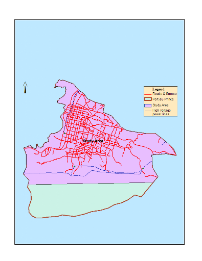
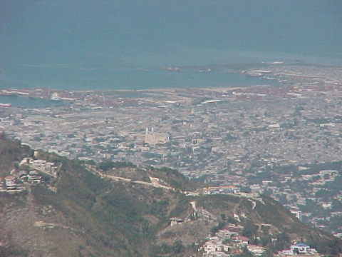
Figure 1: left: Base map of
Port-au-Prince and the study area; right: Port-au-Prince's view from the
southeast hills.
3.2 Data collection
The features included in the dataset derive from two main
sources: a) data readily available from the Remote Sensing and GIS Unit of
Haiti's Planning Ministry (formerly UTSIG, currently CNIGS) and IHSI; b)
digitization of multiple layers from topographic map, scale 1:12,500 prepared
in 1994 by the Defense Mapping Agency, Hydrographic/Topographic Center,
Bethesda, MD. The first source category includes the administrative boundary
of Port-au-Prince, the habitat density, and the land use. The IHSI's SDE
delimitation contributed to the reattribution of the habitat density layer.
Features digitized within an ArcMap interface included: contours, rivulets and
other waterways, high voltage power lines relay-centers and power energy
centrals, the main roads and other high-traffic-density streets, the waste
collection network, formal and informal marketplaces, the main hospitals, the
cemetery, the seashore, and the very important points (VIPs), which are
landmarks found on the topographic map. All the layers were standardized to
UTM projection, NAD83, Zone 18N, unit in meters. As can be seen most of the
features were obtained by the laborious digitization process.
After digitization the features where edited in accordance to
pre-established set of topologic rules in order to ensure the integrity of the
database. Overlaps, dangles, unwanted intersections, wrong attributions, and
any other topologic errors revealed by the topology validation tool were
corrected with the editing tools provided in ArcMap until all the errors were
adjusted.
3.3 Data limitation
During the digitization, attributes were partially collected and
put into the associated tables. In spite of our knowledge of the area, which
we used to fill the gap of missing information on the topographic map, this
task could not be completed. A field data collection would be necessary to
correct this deficit. However due to time and resource limits, this was beyond
the scope of this study. In addition to this, an independent data set would be
required to validate the digitized features. In fact many errors of
digitization inherent to human might have escaped the topologic validation but
without compromising the data integrity. As noticed by Murphy (2005),
digitizing contours... is a tedious and mistake ridden process. Nonetheless we
don't feel that this significantly affected the results of this study.
Essentially, the biggest concern was the lack of data that
restricted the insertion of some important factors in the model. The last
population census was built upon the SDE unit and contains data about the
number of people and other demographic characteristics. Nonetheless, the
format of this data has not been made available to the public. We estimate
that it is an important step toward comprehending the reality at micro-spatial
scale and we strongly encourage researchers to adopt the SDE in future
assessments. Finally, during the data collection process it was difficult, if
not impossible, to discover any national government entity's website providing
access even for purchasing spatial data. The consequence was a loss of much
time and energy that could be allocated elsewhere.
3.4 Construction of the model
3.4.1 Process Overview
The choice of variables affecting environmental health hazards
and vulnerability arises from the literature review, data available for the
study area, and ground-specific reality that might not be in line with any
known theory. Generally, tools such as buffer and Euclidean distance were
applied to measure people's exposure level to the hazards considered. A raster
structure was utilized to facilitate the integration of the multi variables
through Boolean operations and overlay combination. Nine factors were included
in the model and each was assigned a weight between 0 and 1, based on its
relative importance in affecting health. Since we could not access any
specific study providing weights for the study area different weighting
approaches were brought out. The sub-variables contributing to the making of
one factor, such as in the case of traffic pollution, waste pollution, and
pollution from rivulets, were weighted on the basis of our own perception of
their respective importance. Again this approach was used because of lack of
support from the literature.
The entire modeling process was compiled, validated and run
within the ArcMap Model Builder through multiple iterations. The model's
outline and the script of its execution are provided in Appendix C and Appendix
D.
To summarize, the model was generated in four main stages.
1) The first stage consisted of transforming the basic parameters
into factors either by aggregating sub-variables or calculating distance where
applied. The general form of this process is as follow:
Fi = w1*V1 +
w2*V2 + ...+ wj*Vj or Fi
= ?wj*Vj;
with Fi: Factor i; Vj: sub-variable j;
wj: weight of sub-variable j, and
w1+w2+...+wj = 1
2) Subsequently, grids with continuous values were standardized
into discrete values from 1 to 4 using the geometric classification
technique.
3) In the third stage, the factors were aggregated using WLC:
Environmental Health Risks (EHR) = ?Wi*Fi,
where Wi = weight of factor I, and
W1+W2+...+Wi = 1
3) In the final stage the weighted sum of factors was
reclassified into discrete values representing the four risk levels, using four
different reclassification techniques.
3.4.2 Environmental Health
Factors
3.4.2.1 Air pollution from traffic
Vehicular traffic is recognized to be one of the main sources of
air pollution in urban cities. Carbon monoxide, hydrocarbons, nitrogen oxides
are the major air pollutants generated by motor vehicles, and are the underline
causes of lung malfunction, lung cancer, cardiovascular diseases, respiratory
symptoms, stroke, neurobehavioral problems, premature mortality, and possibly
exacerbation of asthma, which ultimately results in deaths (UNEP 1994a, Watkiss
et al. 2000, Maheswaran and Elliott 2003, Nafstad et al. 2003, Greene and Pick
2006). The main roads of Port-au-Prince are associated with high traffic
concentration particularly at peak hours. Wargny (2004) describes the traffic
situation in the downtown area in these terms: «The traffic jam is quasi
permanent. The third-hand vans that provide public transportation spit black
smoke, and the carbon monoxide aggregates to the fecal dust...» Refining
measures of exposure to air pollution takes into account proximity to the
source of pollution (WHO 2005). Other factors that exacerbate pollution
concentration in Port-au-Prince are the occasional maintenance of the vehicles,
the lack or absence of motor vehicle emission control, leaded gas consumption,
and in general the deficient control of cars by the authorities. In addition
to housing close to heavy traffic, which also creates indoor pollution,
commercial activities take place for long hours in the streets. Therefore,
vehicle traffic impact both outdoor and indoor pollution.
Among various approaches, the qualitative method is recommended
to assess the exposure to air pollution from traffic (WHO 2005). Different
studies used a distance analysis approach to model air pollution from traffic
(Elliott et al. 2001, Hoek et al. 2001, 2002, Wilhelm and Ritz 2003, Ferguson
et al. 2004, Schikowski et al. 2005). The final determination of traffic
pollution was built upon the linear combination of four variables: land use,
elevation, traffic density, and distance to roads with high traffic volume.
This approach assumes that there is no spatial variability excluding elevation
within the area and doesn't take into account different coping strategies and
capacity for the households exposed. Likewise the mean level of concentration
and the mean amount of time exposed were used in this model.
Though buffers applied differ from one study to another,
depending on the situation at hand, a Euclidean distance grid was generated to
the main roads and important traffic streets, and distances comprised between 0
and 300 meters were considered in the delimitation of four vulnerability levels
ranging from low to very high. Afterward three raster surfaces were
constructed for traffic density, elevation, and land use. The elevation raster
was derived from the DEM itself created from the contours, the rivulets, and
the VIPs. One thousand points were randomly generated for the study area and
input as location data to be sampled for DEM values. The elevation points
obtained were subsequently converted to raster using the Inverse Distance
Weighting (IDW) within the Spatial Analyst tool. IDW was chosen for its
simplicity of use and the large amount of points that were available for its
creation (1000). Though IDW has the effect of flattering peaks and valleys, the
utilization of the VIPs (representing sample of high and low elevation in the
area) in the DEM surface creation, this disadvantage was minimized.
High risks were associated with distance less than 50 meters,
high traffic density areas, high residential areas and low elevation as shown
on Table 13 in Appendix A. These sub-variables were aggregated using weights
in relation to their assumed implication in creating air pollution. No data,
specific studies or expert opinions were available to support this assumption.
We had to make a personal decision about these weights.
Greater weights (0.4 and 0.3) were assigned to the exposure
factors (distance to road and traffic density) and a smaller weight (0.15) was
applied to the two other factors as seen below:
Traffic Pollution Risk = 0.40*(Distance to Roads) + 0.30*
(Traffic Density) + 0.15*(Land Use) + 0.15*(elevation)
The final step involved reclassifying the resulting grid into
different thresholds using the geometric interval reclassification
algorithm2(*). This scheme
was used for its ability to deal both with the number of values in each class
range and to establish consistent change between intervals (ESRI 1996). More
details are provided in Appendix in Table 14.
Table 1: Pollution from
Traffic - Risk Thresholds
|
Thresholds
|
Low
|
Moderate
|
High
|
Very High
|
|
Range of Values
|
0.9 - 2.3
|
2.3 - 2.9
|
2.9 - 3.3
|
3.3 - 4
|
|
Final value
|
1
|
2
|
3
|
4
|
3.4.2.2 Waste Pollution
The United Nations Conference on Environment and Development
(1992) pointed out that rapid urbanization and demographic concentration have
shocking implications for shelter and sanitation, and especially the disposal
of wastes. Waste is responsible for the transmission of agents of infectious
disease from human and animal excreta, the breeding of disease vectors, and
exposure to toxic chemicals in human and animal excreta (WHO 2006).
Port-au-Prince is the perfect example of this statement. Waste production and
disposal outweigh the institutional, structural, and managerial capacity of
institutions in charge. Two problems arise from waste collection in
Port-au-Prince. First, the collection of waste is absent in slums due to
inaccessibility to the narrow streets and alleys (World Bank 2005). Second,
where it occurs, waste collection is not reliable. For instance, a lack of
fuel or money to buy it, broken or lack of vehicles, and employees' strikes
may cause waste to store up for days, even weeks, spreading all over the
streets, blocking vehicle transport, and giving off offensive smells. In fact
the garbage is fully exposed to the air and the wind, along with mosquitoes,
cockroaches, and rodents facilitating the spatial propagation of the
pollutants. No less shocking is the presence of hogs in some neighborhoods
streets where waste is dumped.
Though these factors could not be accounted in the determination
of waste incidence, we assumed that the spatial extent of this hazard is
inversely proportional to the proximity to the sources. The waste collection
network was digitized based on information gathered from SMCRS (Service
Metropolitain de Collecte des Résidus Solides). The geometry of the
network being linear, we had to consider whether the hazard manifests across
the network or in dumping at specific points. However, no such information was
available: the collection locations may change at any time and, in spite of the
presence of some established posts along the network, there is no way to
control the emergence of new unplanned ones. After calculating the Euclidean
distance of the waste network feature, the resulting raster was divided into 4
classes from 0 to 400 meters with increment of 100 between each threshold.
To take into consideration the inaccessibility of some areas to
waste collection, neighborhoods located at least 400 meters from the waste
collection network were also integrated into the model. In low-to-medium
residential areas where mostly people of middle economic class or above reside,
some private services ensure the pick up of garbage. But people living in
high-to-extremely high density housing neighborhoods may be struggling to get
rid of waste, may have used non-hygienic or non-conventional ways to eliminate
their garbage (for instance burning, or depositing it in the streets when it
rains, or dumping it into the channels) , and consequently create a hazard for
human's health. Those areas away from the network were given values in
reference to the housing density. Then, both distances less than 400 meters
and greater 400 meters were summed.
Regarding the sanitation aspect of the neighborhoods, it would
not be reasonable to assume that the waste network conditions are uniform
everywhere. For instance, in areas involved with intensive commercial
activities like informal markets places, waste production is far much greater
than in areas with little activity. The waste network at La Saline does not
weigh against Lalue's circuit. This consists of a different aspect influencing
waste accumulation and conditions. Based on this evidence a raster that stands
for waste conditions was created and was integrated into the waste factor
determination.
Furthermore, elevation was believed to play a role in
neighborhoods' exposure to waste effects. On one hand, waste from upslope is
carried down by wastewater from the canals and by runoff; on the other hand, in
the absence of an efficient collection system, waste accumulates in lower
elevation and is mixed with water from artificial ponds and obstructed canals.
The same rationale illustrated for the pollution from traffic vehicle may be
also true for waste: better air circulation in higher elevation acts as barrier
to attenuate the pollution's impact of the garbage.
The different factors were aggregated using weights of 0.5, 0.3
and 0.2 for distance from waste collection network, conditions, and elevation
respectively. Once again those weights were personally chosen since I could
not access any example in the literature review for the study area. The result
was standardized to values comprised from 1 to 4 as displayed in Table 2.
Waste Risks = 0.5*Distance + 0.3*(Network conditions) +
0.2*Elevation
Table 2: Pollution from
Waste - Risk Levels
|
Levels
|
Low
|
Moderate
|
High
|
Very High
|
|
Range of values
|
0 - 1
|
1 - 2
|
2 - 3
|
3 - 4
|
|
Reclassified values
|
1
|
2
|
3
|
4
|
3.4.2.3 Public formal and informal market places
Public formal and informal markets are another potential source
of waste and neighborhood pollution. Recent evidence has suggested a close
relationship between the activities of the informal sector and the degradation
observed in the urban environment of Port-au-Prince (Howard 1998). The
so-called public markets contain unspeakable deleterious hygienic conditions
harmful either for the attendants or people living in their proximity. The
informal market places pack the downtown area of Port-au-Prince in a chaotic
manner and at a point that is impossible to delineate its extent. According to
Wargny (2004), everybody attempts to sell something. In the past,
Port-au-Prince had some market places. Nowadays, port-au-prince is a market
place, continuous, insisting, unstoppable, and obsessing.
Market features were digitized both as polygons and points. Yet
the list provided by the communal administration's office was not exhaustive.
Many spontaneous and dispersed markets are established along the streets and
generate tons of waste for which no recovery plans exist. Some of them are the
extended version of a traditional market whose capacity has exploded with the
astounding population increase. The nature of these commercial exchange sites
make it difficult if not impossible to delineate their physical extent and thus
to integrate them in a model.
After calculating the Euclidean distance from markets provided in
the SMRCS' list, point and polygon features were combined using the maximum
function within the single output map algebra tool, and were reclassified as
shown in Table 3 below:
Table 3: Pollution from
Market Places and Risk Levels
|
Threshold distance (meter)
|
Reclassified values
|
|
0 - 100
|
4
|
|
101 - 200
|
3
|
|
200 - 300
|
2
|
|
300 - 400
|
1
|
3.4.2.4 Hospitals and the main cemetery
Though there is not much theoretical support and previous studies
available for validation, another factor affecting neighborhood pollution in
Port-au-Prince is the major hospitals and the central cemetery. Not
integrating them into the model would result in ignoring an important part of
the specific environmental context in the study area. The conditions of
sanitation within and around the hospitals, and more particularly the
Sanitarium and the State University Hospital, make them hazardous and unsafe
places to be exposed for long time. This situation is aggravated first, by the
adjacent location of the mortuary to the general hospital often affected by the
common lack of power to adequately maintain the equipment; second, the general
belief and its concomitant negative impact that, since the type of service is
public, its management will be inefficient. Consequently the level of care
allocated is marked with negligence and falls far below the normal level it
would be in a private structure.
EPA (2005) provides a list of air pollutants that may derive from
hospitals even in normal operating situations. This list comprises mercury,
found for instance in thermometers. Mercury emits toxic vapors that go to the
lungs, and impact the kidneys, liver, respiratory system, and central nervous
system. It can escape into the outdoor through any openings, and even its
incineration doesn't prevent it from reaching the outdoor air. Polyvinyl
chloride, used in plastic products, is another source of air pollution even
when it is incinerated. It emits dioxin, which is a strong carcinogen that
hampers normal reproduction and development even in small amounts.
However, the environment in question in this study area is still
more complex than the normal conditions described by EPA, though quantitative
information is lacking. The sanitation conditions in the main cemetery are
precarious. Thus far the cemetery suffers from overpopulation. Often dead
bodies are exposed to the air for hours to allow new corpses to be buried in
the same grave or in the same hole. Moreover, cases of vandalism and stealing
of fresh coffins are reported, which also expose corpses to the air and
contributes to pollution.
For the cemetery the same distance approach was used to generate
thresholds separated by 100 meters from 0 to 400 meters. Regarding the
hospitals, first buffers from 10 to 100 meters were built in relation to the
comparative sanitation conditions at these facilities. Then the result of the
Euclidean distance on these buffered areas was reclassified into very high risk
(4), high risk (3), moderate risk (2), and low risk (1) using corresponding
distance thresholds of 50, 100, 200 and 300 meters.
3.4.2.5 Housing density
High density housing poses serious threats to human health by
forming sinks for outdoor pollutants, which is aggravated by the fact that the
houses are not well-ventilated (Ezatti et al. 2005, YTV 2007). Housing density
also makes up the primary source of indoor pollution due to unsafe human
excreta disposal, and household fuel consumption (Ezatti et al. 2005).
Consequently these unsafe settlements with poor environmental quality expose
their residents to social instability and communicable and non-communicable
diseases, such as skin and eyes infections, diarrhea, respiratory infections
and environmental hazards (WHO 2001a). Slums populate different locations of
Port-au-Prince's sea coast, built on and in unstable, stinky and unhealthy
waste, in the dust or in the mud. They are called «Brooklyn» or
«Manhattan», using a supreme sense of the sarcasm (Wargny, 2004).
We acknowledge that housing density embodies both aspects of
hazards and vulnerability. Though present as a vulnerability factor in almost
all the variables considered, and acting as the main trigger of the different
risks considered, it was suitable to reduce the redundancy that would result by
adding it each time. We use the term risk for the reason stated above that
housing density represents a factor of air pollution hazard and at the same
time a vulnerability feature. That is, even if there is no other risk factor
present in a location, high and very high housing density are deemed sufficient
conditions for the existence of high risk in these places.
Housing density was originally based on a grid 0.5x0.5 kilometers
in size, which classified density in 6 categories from null to extremely high
(Table 4). Though it was unclear what theoretical background this
categorization was based upon, it was found inappropriate to use it in this
study. A first example of this inconvenience provided in Figure 2 indicates
that extremely high density represents more than 72% of the area, including
slums, commercial and residential neighborhoods. Another illustration is that
the difference between average and very high density is only 6 houses per
km2. Hence it was too general and would not allow us to discriminate
neighborhoods with environmental patterns significant for health assessment.
Then a grid of higher resolution (0.3x0.3 km, Figure 3) was generated. This
was manually reclassified based on SDE count of housing published by IHSI and
with the assistance of a live image from Google Earth, which clearly displayed
the density difference. Table 5 provides a summary of risk levels associated
with different thresholds of housing density.
Table 4: Housing Density
classification in the original grid
|
Values
|
Density Level
|
|
0
|
Null/Very Low
|
|
1
|
Low
|
|
2-5
|
Average
|
|
6-10
|
High
|
|
11-23
|
Very High
|
|
65 - 300
|
Extremely High
|
|
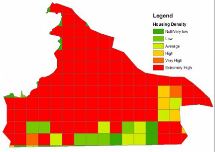
![]()
Figure 2: Housing Density
as classified in the original grid 0.5x0.5 km
|

Figure 3: Housing Density
after reclassification (grid size: 0.3x0.3 km)
|
Table 5: Housing Density and Risk Levels
|
Housing Density
|
Risk Levels
|
|
Low (1-2)
|
Low (1)
|
|
Medium (3)
|
Moderate (2)
|
|
High (4)
|
High (3)
|
|
Very High - Extreme (5-6)
|
Extreme (4)
|
3.4.2.6 Pollution from water
bodies
Urban and peri-urban population health is equally affected by
wastewater from urban drains and municipal dumping of waste, especially human
excreta (Nsiah-Gyaabah et al 2004). River pollution is particularly found to
be worse where rivers pass through cities and the most widespread is the
contamination from human excreta, sewage and oxygen loss (UNEP 1986). Canals
and rivers are also used as an outlet for trash, particularly at locations
where waste collection is lacking. Stagnating water transmits bilharziose or
triggers malaria. Additionally, where potable water is rare, poor people
often use the polluted rivers to wash their clothes, contributing to the
pollution, and exposing themselves to multiple pollution hazards. Lastly,
polluted water bodies represent a source for the breeding of disease vectors
(WHO 2001).
In addition to distance to rivulets, which was classified into
four levels from 0 to 400 meters, slope was integrated as a vulnerability
factor. Low slopes were deemed more favorable to water pooling, mosquitoes
breeding, and a higher concentration of pollutants, therefore correspond to a
higher risk. That is, for the same threshold distance to the channel (e.g. 100
meters) people living in areas located in lower slope were more at risk than
those living on steeper slopes. These two factors were summed with a greater
weight assigned to distance to channels. The result was reclassified with the
geometric interval technique as it appears on Table 6.
Water body risks = 0.7*(distance to rivulets) + 0.3* slopes
Table 6: Pollution from
water bodies - Risk Levels
|
Distance(0.7)
Slope (0.3)
|
>200
|
101-200
|
51-100
|
0-50
|
|
1
|
2
|
3
|
4
|
|
> 25%
|
1
|
1.0
|
1.7
|
2.4
|
3.1
|
|
15 - 25%
|
2
|
1.3
|
2.0
|
2.7
|
3.4
|
|
5 - 15%
|
3
|
1.6
|
2.3
|
3.0
|
3.7
|
|
0 - 5%
|
4
|
1.9
|
2.6
|
3.3
|
4.0
|
|
Risk Levels
|
|
1 - Low
|
2 - Moderate
|
3 - High
|
4 - Very High
|
|
1 - 2.4
|
2.4 - 3.05
|
3.05 - 3.35
|
3.35 - 4.0
|
3.4.2.7 Proximity to the sea
The area immediately contiguous to the seashore is the last
repository for all type of waste, mud, household and human refuse, and
industrial waste. In developing countries, people in poor households living in
proximity to the sea and who do not have a toilet or latrine don't
have any other alternative than to unload their defecation either in
the sea shore or vacant plots and open drains (Olanrewaju 1990). In
addition, discarded cans, bottles, waste incoming from all activities are sinks
and places for mosquitoes breeding, which spread diseases such as malaria and
dengue (SKAT 2002). In Haiti, as reported by UNEP (1996), several shantytowns
have been built in proximity to the seashore in recent years. Some of them are
erected on dumping sites which often block water flowing to the sea, and
generating ponds. The wind blowing from the sea may dissipate the effects of
pollutants or it may spread them across a larger area. These locations have a
high dose of pollutants and expose their residents to very harmful effects. A
2001 Panamerican Health Organization (PAHO 2001)) report on health in Haiti
stated that the transmission of malaria occurs mainly in coastal areas
coincident to altitude lower than 300 meters.
A Euclidean distance surface was calculated with a threshold of
1000 meters from the sea divided into four vulnerability levels as shown in
Table 7. The impact may not be linear and may vary in function of some factors
such as the disposition of the slums, local variation in elevation,
canalization or conditions of the canalization (which is a temporal variable),
amount and types of debris (vehicle carcasses for instance may block the
movement of waste towards the sea), etc. For simplicity, we assumed that the
phenomenon is linear in its materialization.
Table 7: Distance to the
sea and Risk Levels
|
Distance (in meters)
|
Risk Level
|
|
0 - 300
|
4
|
|
301 - 500
|
3
|
|
501 - 700
|
2
|
|
> 700
|
1
|
3.4.2.8 Proximity to high voltage power line
Power lines are considered a noticeable source of electromagnetic
pollution to which extended exposure to some specific frequencies may result in
cancer, birth defects, decreased immunity to disease, even new sicknesses
(Michrowski 1991). A study conducted by Fews et al. (1999) observed an
increased exposure to pollutant aerosols under high voltage power line. But
another study conducted by Draper et al. (2005) and leading to the conclusion
of association between the proximity of birth residence to high voltage power
lines and children with leukemia (e.g.) has been the occasion of much debate
(Day et al. 2005).
The delineation of this hazard was built on a uniform buffer of
500 meters from the power cables (line geometry) and 1000 meters around the
distribution centers (point geometry). The distance ranges considered are
shown in the Table 8.
Table 8: Distance to High
Voltage Power Lines and Vulnerability level
|
Distance to Lines (in meters)
|
Distance to Centers
|
Vulnerability Level
|
|
0 - 150
|
0 - 300
|
4
|
|
151 - 300
|
301 - 500
|
3
|
|
301 - 400
|
501 - 700
|
2
|
|
> 400
|
> 700
|
1
|
Both distances were combined using the max function within the
single output Map Algebra tool. In areas where the two grids intersect, the max
function assigns the greatest value to the output grid. The use of this tool
was necessary to put in evidence extreme cases of risk.
3.4.3 Linear Combination of
the Variables
The Expert Opinion survey was conducted with the participation of
ten local professionals having a certain familiarity with health and
environmental issues in the study area. The respondents comprised 5
professionals in public health, 2 in environment, 2 economists and one
agronomist. They were requested to assign a score from 1 to 9 (with 1 being
very low and 9 very high) in order to rank the relative importance of the
environmental variables of the model (see results in Table 15 of Appendix A).
The ten scores were summed for each factor and divided by the total scores for
all the factors. This provided a normalized weight comprised between 0 and 1.
Hereafter this approach will be referred to Expert Opinion Weighting (EOW).
The second weighting approach assumed equal influence of the
factors on health risks and assigned the same weight of 1/9 to each. The last
weighting scheme was based on our own perception of the spatial extent and
intensity of the different hazards of the model. Henceforth, either of these
designations will be used for this approach: Own weighting or personalized
weighting. Finally, to put in evidence those areas exposed uniquely to high
risks for any factor, the maximum combination was applied. The max operator is
a local function within the Spatial Analyst tools, which uses several input
rasters to calculate the highest value on a cell-by-cell basis within the
Analysis window.
Further the linear regression technique was used to validate the
rationale under the Expert Opinion weighting and the personalized (own)
weighting scheme. The intent was to discover the degree of correlation existing
between the assigned coefficient in these two schemes and the factors in terms
of area covered and the proportion of high and very high risks.
3.4.4 Classification Schemes
The final classification was implemented with four classification
techniques namely, Quantile, Natural Breaks (or Jenks), Equal Interval, and
Geometric interval. To compare the linear combination methods, the results
provided by these classification algorithms were averaged and compared to
another manual classification (we call it standardized classification). This
process was utilized to isolate the effect of a given classification scheme.
The manual classification regrouped the features into four discrete classes 0
-1, 1 - 2, 2 - 3, and 3 - 4 representing the four risk levels.
3.5 Model's Summary
Here are the four combination schemes employed to aggregate the
environmental health risks factors considered in the model.
1) Expert Opinion Weighting (EOW)
EHR = 0.13(Traffic Pollution) + 0.14Waste + 0.08(cemetery +
hospitals + High Voltage Power) + 0.13Markets + 0.13(Housing Density) +
0.12(Polluted water) + 0.11(Distance to the sea)
2) Own Ranking
EHR = 0.14(Traffic Pollution) + 0.16Waste + 0.06(Distance to
Cemetery + Distance to the Hospitals) + 0.10*(Distance to market places) +
0.14(Housing Density) + 0.10(Pollution from Streams) + 0.16(Distance to the
sea) + 0.08(High Voltage Power)
3) Equal Weight
EHR = 0.1111*(Traffic Pollution + Waste + Distance to Cemetery +
Distance to the Hospitals + Distance to markets places + Housing Density
+.Pollution from Streams + Distance to the sea + High Voltage Power)
4) Maximum output
EHR = Max(Traffic Pollution, Waste, Distance to Cemetery,
Distance to the Hospitals, Distance to markets places, Housing Density,
Pollution from Streams, Distance to the sea, High Voltage Power).
3.6 Sensitivity
Analysis
The spatial model presented in this study is defined by a series
of input factors, parameters, variables, weights, and combination techniques
subject to many sources of uncertainty. These sources comprise lack of data,
insufficient support of literature review for the study area, and error of
measurement, and weight attribution, which impose limit on our confidence in
the output model. The range of alternatives available in implementing the
overlay provides the flexibility to come to any desired conclusion (O'Sullivan
and Unwin 2003). Therefore, it is important to evaluate our confidence in the
model and assess the uncertainties associated with the modeling process and
with the output. A sensitivity analysis evaluates the effects of modifying one
or several input parameters on the model output (Akçakaya 1996, Franklin
et al. 2002) and examines the overall variability in the possible output
(O'Sullivan and Unwin 2003). The weight of factors believed to be of greater
magnitude in the model such as traffic and waste pollution was modified while
adjusting the coefficient of the other variables to keep the total sum of the
weights to 1. Three different scenarios were assessed. First, using the
weights obtained from the expert opinion survey as basis, the coefficient of
traffic pollution was increased from 0.13 to 0.3. Second, the weight of waste
pollution was increased from 0.14 to 0.3. The last approach was to allocate
weights in proportion to the area extent of each factor. We observed the change
in proportion occurred between the four risk levels and compared the arithmetic
sum of changes in the three cases to determine the sensitivity of the model.
4 RESULTS AND DISCUSSION
The results of this modeling exercise are divided into three
sections: the first section presents the summary results of the model as a
whole along with the different aggregation and classification schemes; then
statistics are shown for the multiple factors that make up the model; finally,
the effect of changing one assumption about the model is analyzed.
4.1 Results by Linear Combination Schemes
Participants in the Expert Opinion survey ranked waste as the
major source of pollution (0.14) above traffic, markets and housing density,
which equally came second with a weight of 13%. A lesser weight was allocated
to cemetery, hospitals, and high voltage, which accounted for 8%. Indeed, the
largest gap between the factors' weight was at most 6%.
4.1.1 Expert Opinion Survey, Equal Influence (Equal Weight),
and Personalized Weightings
Irrespective of the combination or the classification
technique used, about 41% of the study area was found exposed to high and very
high environmental health risks, all factors considered. This result was
brought out by simultaneously averaging the Expert Opinion survey, the equal
influence, and the personalized combination schemes on one hand, the quintile,
the natural breaks, the equal interval, and the geometric interval techniques
on the other hand, so that this number is freed of the influence of any single
combination method or classification technique. The averaged results are
displayed in the table below. A more complete set of results is provided in
Table 16 in Appendix A.
Table 9: Percent of areas
per vulnerability level - Average score for the four classification
techniques
|
Combination scheme
|
Very High
|
High
|
Moderate
|
Low
|
Total
|
|
Expert Opinion
|
15.6
|
25.4
|
35.9
|
23.1
|
100.0
|
|
Equal Weight
|
14.4
|
21.6
|
38.3
|
25.7
|
100.0
|
|
Personalized assignment
|
14.9
|
25.9
|
36.5
|
22.7
|
100.0
|
|
Average
|
14.9
|
25.9
|
36.5
|
22.7
|
100.0
|
The standardized classification scheme, which terms as a control
(Table 10), led to a far different result with no areas exposed at very high
risk and at most 15.9% of areas with high risks. In both cases the largest
percentage was found in the category moderate risks, which amounts up to 59.3%
in the standardized classification versus 36.5% in the first case. This
perceptible discrepancy brings forward how the analysis built on one or another
technique may lead to erroneous conclusions.
Table 10: Percent of areas
by risk level and aggregation scheme using a standardized
classification
|
Combination scheme
|
Very High
(3-4)
|
High
(2-3)
|
Moderate
(1-2)
|
Low
(0-1)
|
Total
|
|
Expert Opinion
|
0.0
|
16.6
|
60.2
|
23.2
|
100.0
|
|
Equal Weight
|
0.0
|
11.7
|
59.7
|
28.6
|
100.0
|
|
Personalized assignment
|
0.0
|
19.5
|
58.0
|
22.5
|
100.0
|
|
Average
|
0.0
|
15.9
|
59.3
|
24.8
|
100.0
|
Comparing the three methods used to combine the multiple factors,
EOW and the personalized approach provided very similar results displaying a
maximum difference of 0.7% for areas at very high risks (Figure 4). Whereas
the gap between the EOW and the personalized weighting was minimal, a greater
percentage (maximum 4.3%), discriminated them from the equal influence
technique. The equal weighting technique was prone to assign more cells in low
and moderate levels and consequently promoted the influence of low values over
high values than did the two other techniques. Despite this difference the
general trend showed a larger percentage of areas at moderate and low risk
irrespective of the classification technique utilized, as it appears on the
figure below. What may explain this?
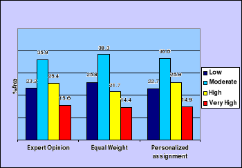
Figure 4: Environmental
Health Risks -
Average percent of areas by combination
scheme
Most of the parameters did not have a spatial domain covering the
entire area. The average area extent for all the parameters was 52%, with only
housing density having 100% assignment. For a given factor, areas with no risk
participating in the combination reflect on the result. Large scores (values
greater than 3) can be obtained only if the largest possible number of cells
participating in the combination contributes with a maximum score. In other
words, the various factors considered are dispersed over the area of study with
few cases of high value overlap. Since the equal weighting method does not
discriminate the variables, the final grid calculation was heavily affected by
these zeros. This fact is evident in the standardized classification technique
which established the classes based on discrete values at fixed interval. The
category 4 (values ranging from 3 to 4) was virtually absent in all the
combination schemes.
The map displayed on Figure 5 results from the EOW combination
using the geometric interval reclassification technique. It indicates a
concentration of high risk areas in the downtown area and heading toward the
coast. Conversely, areas at moderate and low risks are located away from the
downtown toward the periphery mostly made of high slopes. This observation
confirms the assertion that high population density associated to untidy
urbanization in a context of weak institutional framework is mainly responsible
for the daily occurrence of life-threatening hazards.

Figure 5: Environmental
Health Risks in Port-au-Prince - EOW classified with the geometric interval
technique
4.1.2 The Maximum Weighting Scheme
The maximum weighting scheme so far was not taken into
consideration in the previous discussions since it has a different connotation
and could not bear a reasonable comparison with the other approaches. This
function tends to maximize risk. Because of this a high percentage, 92.5%, of
the area was found exposed at high and very high risks for all the hazards
combined, which is a huge contrast to the results above. In this approach,
since no weight was allocated, the cell with the biggest value rules over the
others. Simply put, the result signifies that for this specific cell, there is
at least one health hazard whose risk level corresponds to this maximum value.
This method was chosen intentionally so as to bring forth the diversity of high
risks prevailing in almost the entire area (Figure 6). This situation also
reveals the lessening of individual factors' significance in aid of the
collective importance of the model. Policies interested rather in solving
environmental problems that arise from a specific field may find this approach
more attractive and more practical.

Figure 6: Environmental
Health Risks in Port-au-Prince - Maximum combination technique using the
Geometric Interval classification method
This approach also outlines the specific location and extent of
each hazard considered. For instance, someone accustomed to the area can
clearly notice the path of high voltage power lines and the prism of risks in
its neighborhood. Likewise, pollution associated to the proximity of the sea
and of vehicle traffic is obvious.
The opposite procedure consisted of determining whether some
areas were exposed simultaneously at high risk for all the hazards overlaid. A
conditional statement was performed to superimpose all the areas where the
conditions «high risk and very high risk» were met. This situation
was not present in any area. This might be because of the spatial dispersion of
the factors over the entire area.
4.2 Comparison of the Classification Techniques
This section presents a comparison of the performance of the
classification methods, namely quantile, natural breaks (Jenks), equal
interval, and geometric interval, in distributing values among risk levels.
Once again to attenuate the effect of the combination schemes, the scores of
each classification were averaged for the 3 approaches. A summary of the
results is displayed in Appendix A, Table 17, while Figure 7 facilitates the
comparison of the distribution of the area among the four risk stages.
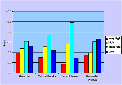
Figure 7: Environmental
Health Risks in Port-au-Prince - Percent of area at-risk by classification
technique
Two different patterns are exhibited regarding the distribution
of risk levels. First, whereas the maximum gap among risk levels is very
important for Natural Breaks and Equal Interval (21 and 41%), the Quantile and
the Geometric Interval techniques show a maximum difference of 16%. The second
pattern relates to the cluster of values in opposite categories (low and high).
In this regard, though all the classification techniques have a higher
proportion of values classified as low and moderate risk, equal interval and
geometric interval place a smaller proportion of areas in high and very high
risk (36%) than do Quantile and Natural Breaks (43% and 41%). The former
techniques appear to be pessimistic while the latter is rather optimistic. The
intent of this observation is not to generalize the comparison. This result
might depend on the specific distribution of values and the way these values
were classified beforehand. A visual comparison is offered in Figure 8 and
Figure 9.
For this specific study, if the goal was to highlight the
severity of environmental health risks, the Quantile or the Natural breaks
methods would be appropriate. Conversely, Equal interval or Geometric interval
would be suitable to provide a certain sense of environmental stability and
improvement.
|

Figure 8: Environmental
Health Risks - Own weighting scheme using the quantile technique: greater
proportion of high/very high risks
|

Figure 9: Environmental
Health Risks - Own weighting scheme using the geometric interval technique:
smaller proportion of high/very high risks
|
These discussions and the analysis of the combination schemes
made above illustrate the influence the choice of a specific model or technique
can have on the final results. These results can be manipulated in a certain
way to respond to decision makers' willingness to impress either about assumed
progress accomplished by an implemented project or to attract funding for a
prospective project by drawing a somber cliché of the state of the
environment. As suggested by Osaragi (2002), the selection of a classification
method depends on the nature of data and what we want to communicate about
data.
4.3 Neighborhoods Exposed at High Risks
Another important step was to focus on areas identified as highly
prone to environmental health hazards and assess their most salient
characteristics. While we can't display here all the combinations for the
different schemes, only the results obtained with the personalized weighting
scheme coupled with the natural break (chosen randomly) are displayed in Figure
10.
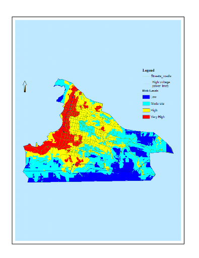
Figure 10: Environmental
Health Risks in Port-au-Prince: Percent of areas at-risk using the Own
weighting scheme and the natural breaks classification method
Twenty two percent (22%) of areas was found overlapped for high
and very high risk from one aggregation method to the other. That is, these
areas always presented high risks irrespective of the approach used to combine
the nine factors. This forms a space of certitude about the results. Most of
these areas are located in the downtown neighborhood and include all the shanty
towns. In particular these areas are well known for high traffic volume, high
population density (so housing density), are located in neighborhoods of public
facilities such as markets, hospitals, cemetery, in low elevation and near
water bodies and the sea coast. These neighborhoods deserve the greatest
attention from the government and/or the non-governmental agencies for
interventions aimed at preventing or lessening impacts on health resulting from
these identified hazards. The complete list of figures is provided in Appendix
B, Figures 21-37. Through these maps the same geographic pattern can be seen
for the different techniques considered. The differentiation, mainly
quantitative, is not substantial.
4.4 Environmental Health Hazards
Table 18 in Appendix A and Figure 11 present a synopsis of the
results by health hazard included in the model. As can be seen, waste
pollution portrays the factor whose severity reaches the greatest physical
extent, 53.4% of high and very high risks. Following this were pollution from
streams (49.1%), high density housing (45.7%), and traffic (42.1%) (Table 18,
Appendix A). The ranking of six factors coincides both for the percent of area
covered and the proportion of area at high and very high risks. This would
indicate a strong association between the physical extent of the factors and
their perceived strength. Indeed the correlation coefficient between these two
outputs exceeds 0.98. Correlation between EOW and Own weights over these two
results was also tested. This yielded to a coefficient of regression
(R2) of 41% (Table 20, Appendix A) and 33% (Table 21, Appendix A)
when running successively single regressions of the EOW (column 2, Table 19)
and the own weighting (column 3, Table 19) over the proportion of high/very
high risk areas (column 6, Table 18). For both regressions the t-statistic was
insignificant at 95% confidence limits and the p values significantly greater
than zero. This result would suggest that the weight assigned by the experts
had little to do with the perceived strength of these hazards. Similarly, when
we ran a regression with the percent of study area covered by each factor
(column 4, Table 19) as independent variable, correlations of 46% and 35% were
found respectively for EOW and Own weighting with the t-statistic significant
and p values acceptably low (close to zero) (see regression results in Tables
22 & 23, Appendix A). This would signify that the experts' judgment and our
perception were more correlated to the physical extent of health hazards, which
can be more easily quantified, than the perceived influence of those hazards.
Although the participants in the expert opinion survey were not cautioned to
provide their rankings based on the physical occurrence of these hazards, this
result implies that this characteristic had to a certain extent influenced the
weight the respondents attributed. Consequently, the experts did a better job
than us in ranking the factors.
If we were to average the results obtained by individual factor,
52% of the study area would be at risk at all levels, of which 47% at high and
very high risk. However, what these percentages did not unveil is the
population exposed, though housing density is an unambiguous surrogate of
population. Applying the 47% rate on the total population would be misleading
since the areas at high risk are also the most populated. Not only are
locations with high and very high housing density inherently exposed to high
risks, the superimposition of low and moderate housing density areas to any
other hazards where the vulnerability is high induces a high risk for the
populations living in these areas. This was one of the issues the maximum
approach attempted to address. Endless combinations could be done to put in
evidence the severity of health risks in the study area. But for now, let's
look at individual hazards and their associated risk levels.
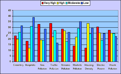
Figure 11: Factors
affecting environmental health in Port-au-Prince.
Percent of area by risk level
4.4.1 Traffic Pollution
Vehicle traffic forms a major source of indoor and outdoor air
pollution in the study area. It is due to high population density that exposes
both, to an increasing number of public and private vehicles using road
surfaces not designed for this volume of traffic, and to the disorganized
development of informal commercial activities which take over the streets. In
addition to these environmental and physical settings, conditions of
maintenance, regulation, and controls of the vehicle fleet exacerbates
pollution. Nevertheless there is no obvious sign of concern either from the
exposed population or from the entities in charge of the environment and
traffic regulation and management, or again public and private organizations
promoting health.
As displayed on Table 18 in Appendix A, about 76% percent of the
area was found exposed to low to very high pollution risks. Neighborhoods with
high and very high risks accounts for 42% of the study area while low and
moderate risk amount to 13% and 21% respectively. The north-northeast section
of the map displayed in Figure 12 makes abstraction of high traffic activities
in some sections of Delmas Road adjacent to the border of Port-au-Prince. Only
when Delmas Road intersects or crosses the border of the study area risks
originated from this road appeared in the analysis. Nevertheless, most of this
boundary section was found prone to high risk from traffic pollution.
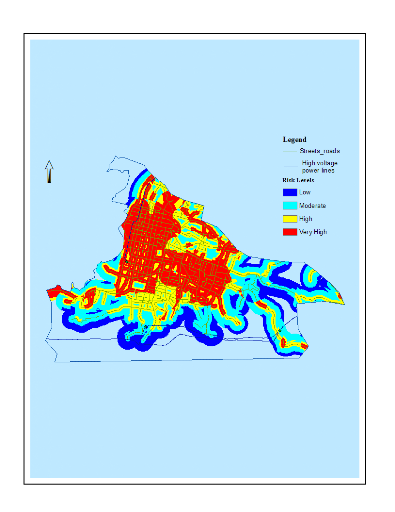
Figure 12: Risks of traffic
pollution in Port-au-Prince
Waste Pollution
We must concede that the modeling of zones susceptible to waste
pollution hazard was arduous. Though the final approach adopted was not
completely satisfactory and necessitates scrutiny, the assumptions made and the
mechanisms developed were likely to provide results that are coincident to the
reality of waste, which is wide spread over the study area. This factor covers
more than 95% of the area and received the greatest weight in the EOW survey.
About half of the study area (53%) was found exposed to at least high risks,
which pinpoints to the severity of this issue and the challenge it poses to
decision makers particularly in a context of very dynamic demographic
variables, and in a setting of weak institutional capacity of management.
Figure 13 shows that neighborhoods away from the collection
network but having high density housing, and those very close to the network
but again with high density housing and located in lowlands were found to
exhibit the highest risk to waste pollution. Conversely people living in high
elevation and where the density of houses is relatively low enjoy a better
environment.
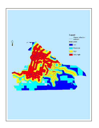
Figure 13: Waste Pollution
in Port-au-Prince
4.4.3 Housing Density
Housing density was deemed one of the most important factors,
which not only embodies a source of pollution and serves as sink for other
sources, but also underlines vulnerability to all the hazards considered.
Though concessions were made to classify some areas at low density where they
would be considered medium-to-high density by international standard
classification, about 46% of the areas were estimated to be high-to-extreme
density (Figure 14). However these densities are unique and incomparable to
those found in developed countries' urban neighborhoods. To illustrate this
sharp contrast, an average of 10,583 homes by square kilometer was counted in
Port-au-Prince by IHSI in the last national census (IHSI 2003). Even more
striking was the maximum density of more than 164,500 dwellings found in one
district. As a result the ventilation is very poor inside and outside these
structures; the distance between the toilets and the living spaces is
negligible, a situation that constantly exposes people to nearly physical
contact with feces and its manifestation; cooking with charcoal is done inside
or adjacent to the house; the effortless transmission of bacteria through
insects, rodents, and cockroaches and many other impacts for the physical and
the mental health.
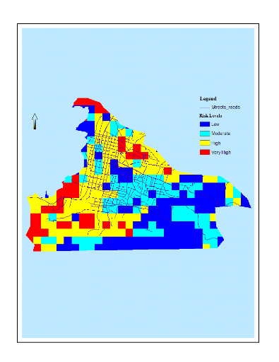
Figure 14: Housing Density
in Port-au-prince
4.4.4 Pollution from Market Places
A common phenomenon that escapes authorities' control in the
study area is the extension of public markets beyond their original assigned
location. This expansion in Port-au-Prince resembles water run-off quickly
turning to overflows due to excess above the retention capacity. It has become
impossible to delimit the physical extents of the market places. In addition
to the official markets, there are the informal markets that have been accepted
as a fact. This study covered only those recognized by the city's
municipality. From low to very high, the hazards they represented formed more
than 22% of the area, of which about 36% (8% in total) where at high to very
high risk (Figure 15). The buffer built around the markets assumes that the
polluted air shed spreads homogeneously in all direction without consideration
of wind direction, transmission vectors traveling patterns, and obstacles in
the vicinity.
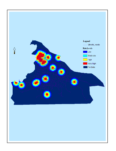
Figure 15: Pollution from
market places
4.4.5 Pollution water bodies
Though the study area is not crossed by any major stream, the
topographic map exhibits multiple rivulets including some with uncertain
physical destination. They might have been relayed by mechanical pathways
built purposely in an urban drainage plan, or obstructed by unexpected
obstacles that make it difficult to determine their conduit. Regardless of the
situation at hand, it represents a serious source of pollution representing the
receptacle of all kinds of municipal waste, and as such poses serious concerns
for health.
As reflected in the model, the total extent of pollution from
water was about 88% of which 56% was at high and very high risk, 18% moderate,
and 26% at low risk (Figure 16). The modeling of these areas integrated slope
to account for the accumulation factor across the path down to the sea and also
the likelihood of water pooling at low slopes atop of high slope. As can be
seen on the map less areas in high elevation were exposed to high risk.
However, neighborhoods in low elevations and even not near channels experience
high risks.
A large part of the downtown area was not part of this assessment
as shown on the light blue section in the northwest. This was because ponds
and water pooling in canals could not be precisely digitized. However this
area is known for poor drainage and channels obstruction by waste, which allow
very unclean water to flow on the streets.
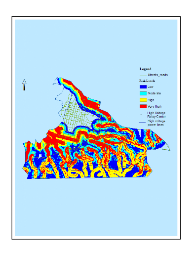
Figure 16: Pollution from
Water bodies
Once again, rivulets that flow near the border of the study area
but that did not cross or intersected the area, were not included in the
determination of this hazard, though they might have had a partial impact.
4.4.6 Pollution from the coast
Pollution incoming from the sea encompasses about 23% of the
study area, among which more than half is at high and very high risk (Figure
17). This area is the densest in term of habitat and traffic, and hosts most
of the slums, commercial activities, some formal and informal market places.
In addition, it comprises the path of one branch of high voltage power line as
well as a power distribution center, and the cemetery and some of the hospitals
are also located close to this area. Consequently it is deemed as one of the
most unsafe neighborhood to live. Nevertheless, as noticed above, this is the
area with the densest population. Any sanitation, urban conversion program,
dislocation and relocation program, health intervention, should initiate in
this area located in the storm's eye in term of environmental health risks.
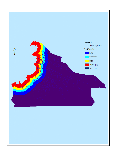
Figure 17: Pollution from
the sea coast
4.4.7 Pollution from high voltage electric power
This hazard was mainly identified along transects in the south
and the northwest section and extended over more than half of the study area.
Neighborhoods under high and very high risks represented over 30% of the total
area. However, though the high and very high risk of the south section of this
hazard is very obvious on Figure 18, it did not appear on the result of EOW
combination. The EOW combination weakens its impact by the fact that part of
this area is isolated in high elevation and low housing density and poorly
influenced the combination. This underlines the importance of approaching the
analysis of the factors both globally and individually.
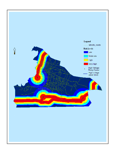
Figure 18: Pollution from
high voltage power
4.4.8 Pollution from the hospitals
Buffers of different sizes were applied in relation to the size
and the level of care used at the hospitals. This information was gathered
from health professionals accustomed to these facilities. The hazards they
represent account for more than 7% of the study area, of which only 30% was
considered at high to very high risk (Figure 19). This low percentage was
expected because of the small buffer applied around three out of 5 hospitals.
Nonetheless the high rate of low and moderate risk levels does not mean absence
of risk, yet a direct measurement of pollution concentration within this
delineation is required.
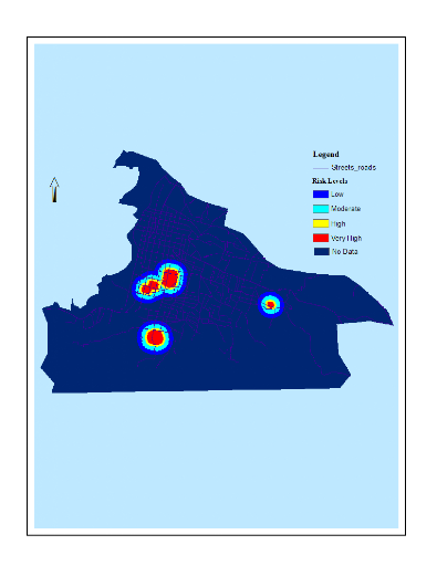
Figure 19: Neighborhood
pollution from Hospitals
4.4.9 Pollution from the cemetery
This hazard represents the smallest in terms of area extent: 4%
of the entire area. High and very high risks were identified in less than 2%
of the study area (Figure 20). However, as mentioned earlier, it is believed
that a reasonable extension of the buffer westward would result in a greater
physical incidence. We assumed that this part was partially covered in the
pollution from water bodies, traffic and waste pollution. An inspection of
these maps at the west side of the cemetery confirms this hypothesis.
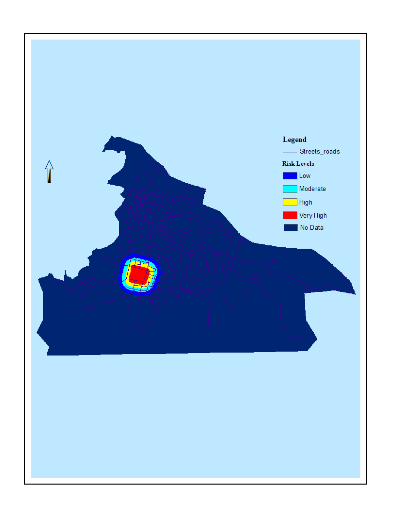
Figure 20: Neighborhood
pollution from the central cemetery
4.5 Sensitivity analysis
Though the comparison of the different aggregation schemes
constitutes a sort of analysis of sensitivity, this section introduces a more
in-depth consideration of this issue. To keep the comparison of the results
as simple as possible, reference was made only to the Expert Opinion weighting
using the geometric interval classification. The maps are displayed in
Appendix B, Figures 38 to 40.
Traffic Pollution Influence
The assumption of an increase of traffic pollution's weight to
30% results in decreasing the coefficient of all the other parameters of the
model while keeping the total weight to 1. Table 11 shows a substantial
alteration of the percent area in each risk level. The most significant change
was observed in the lower risk level which declined by 67%. At the opposite,
high and very high risk levels increased by 50% and 77% respectively. The
overall change is almost 60%. This reveals the strong influence traffic
pollution has on health risk in the study area. To this regard, traffic
pollution represents one of the most urgent issues that policies should
address. Let's recall that traffic pollution occurs in about 76% of the study
area.
Table 11: Increase in
traffic pollution weight compared to EOW
|
EOW
|
Increase in
Traffic weight
|
Difference (%)
|
Absolute
Difference
|
|
Low
|
36.0
|
15.8
|
-56.1
|
-20.2
|
|
Moderate
|
27.1
|
24.0
|
-11.5
|
-3.1
|
|
High
|
19.3
|
29.0
|
50.2
|
9.7
|
|
Very High
|
17.7
|
31.3
|
76.8
|
13.6
|
|
Sum of changes
|
|
|
59.4
|
|
Waste Pollution Influence
The geographical incidence of waste represents 95% of the area.
With the alteration of waste coefficient, the model records a decline in low
classes of about 54% while high and very high risk levels indicate a positive
joint change of 100%. The aggregate change is 45%, 15 points smaller than
changes induced by traffic pollution, though the physical occurrence of waste
is greater than traffic pollution (Table 12). Nevertheless, this influence on
the model is still substantial.
Table 12: Increase in waste
pollution weight compared to EOW
|
EOW
|
Increase in
waste weight
|
Difference (%)
|
Absolute
Difference
|
|
Low
|
36.0
|
19.1
|
-46.9
|
-16.9
|
|
Moderate
|
27.1
|
25.2
|
-7.0
|
-1.9
|
|
High
|
19.3
|
32.9
|
70.4
|
13.6
|
|
Very High
|
17.7
|
22.8
|
28.8
|
5.1
|
|
Sum of changes
|
|
|
45.3
|
|
4.5.3 Proportional Spatial Incidence of the factors
This weighting, brought out based on the relative physical extent
of each model's parameters, assigned a greater coefficient to housing density
(0.21), followed by waste (0.20), rivulets (0.19), and traffic pollution
(0.16). Unlike the previous two scenarios, the area incidence of high and very
high risk levels increased only by 60% and the aggregate change is less than
30% (Table 13). This weighting shrank the gap between risk levels and enables
a better balanced distribution than did EOW.
Table 13: Comparison of EOW
and Proportional Incidence Weighting Results
|
EOW
|
Proportional
Weighting
|
Difference (%)
|
Absolute
Difference
|
|
Low
|
36.0
|
23.8
|
-33.9
|
-12.2
|
|
Moderate
|
27.1
|
27.0
|
-0.3
|
-0.1
|
|
High
|
19.3
|
31.3
|
62.2
|
12
|
|
Very High
|
17.7
|
17.9
|
1.1
|
0.2
|
|
Sum of changes
|
|
|
29.1
|
|
To summarize, the alteration of some of the coefficients of the
model's parameters influenced the results in different ways. The increase of
the traffic pollution weighting had the greatest impact on the model, altering
drastically the categories' rank from top to bottom. This exercise definitely
illustrates the responsiveness of the model to changes of its parameters.
5 CONCLUSIONS
This study took place in a context of unavailability and/or
inaccessibility of data. Even the basic spatial information could not be
obtained from official sources on the Internet. The web pages of the
institutions in charge of the production and distribution of spatial data, or
information in general were projected to be constructed soon or were under
perpetual construction. It took a great amount of effort to generate most of
the features through a long and arduous process of digitization of most of the
data. Often assumptions had to be made to avoid having to collect more data.
The difficulties encountered reveal the requirements for a greater flexibility
of data exchange conditions between institutions, and between institution and
the public, as well as the needs for a better integration of spatial data
available. Furthermore, it is a pressing demand to produce geographic
information at higher resolution in a way to enable researchers to address
issues at the level of communities. Very general spatial information can not
lead to anything but this congenital practice of confounding semantics and
pragmatism. Information, particularly in such disinherited and poor
environment as Haiti, may not be used to confer power to individuals or
institutions. Rather it may constitute a power to promote changes starting at
individual and community levels. We advocate cost efficient strategies to
produce spatial data and make them available to anyone anywhere through the
Internet, even for purchasing.
This study, a first of its kind for Port-au-Prince, attempted to
delineate at-risk neighborhoods for nine environmental health hazards. Though
traditionally the focus has been oriented toward natural hazards, which in
nature are more discreet and whose manifestation leads to direct observation
and quantification, this study reveals that health hazards are not a mental
invention. These hazards are continuous, constant, perilous, and daily affect
a large part of the population. The lack of information and the complexity
posed by quantitative assessment must not lead to the minimization or the
abstraction of such a precarious and deadly phenomenon. This work may
represent a first geographic inventory of environmental health-related hazards
in Port-au-Prince. By relating its occurrence to the underlying causes, it
offers the ability to intervene in specific areas and targeting a specific
factor. To this respect, we strongly encourage the use of the SDE as a
suitable spatial study unit for the collection of data pertaining to a large
array of fields. This approach can strongly facilitate the insight of phenomena
at small community level and promote participation.
High housing density, traffic, waste, streams, and the sea coast
represent the main sources or pollution in Port-au-Prince. However the impact
of the other sources must not be overlooked. They are very serious in the
specific environment and institutional setting of Port-au-Prince.
While the geographic delineation of the hazards may not be exact
in its spatial shape and extent, one confidence remains: the issues addressed
exist and exist in the neighborhoods indicated. Without any field data the
categorization brought out by the ordinal approach remains subjective and
depends on the researcher's perception of the reality under study.
Nevertheless it has the merits of pinpointing areas where environmental health
risks might reasonably be incident and offers the ability to make different
assumptions and adjusting the results on the fly. Various combination and
reclassification techniques likely to influence the output were assessed and
demonstrated the high sensitivity of the model to change in its parameters.
As a specific outcome of this study, the prime interest of any
program aiming to reduce population's vulnerability to health hazards should
focus on these areas identified as at very high risk. They are located
particularly in neighborhoods with very high housing density, which also host
an array of other environmental hazards such as air pollution from traffic,
waste, water bodies and the coastline. By relating these risked areas specific
hazards that threaten them the strategy to adopt becomes less ambiguous.
This study is not complete without a ground truth survey
consisting of collecting information and taking specific measurements on
various pollution factors included in the model. Very limited in time, budget
and other resources, the scope of this study would not allow such
investigation. Information gathered on the field not only would allow
validating the results but equally would enable establishing strong rationale
for hazards delineation and vulnerability scaling. At least the outcome is
deemed a first but important step by defining specific area where distinct
interventions can be done.
APPENDIX A - TABLES
Table 14: Risk of Air
pollution from traffic - Vulnerability scales
|
Roads
|
Land Use
|
Traffic Density
|
Elevation
(meters)
|
|
Distance
|
Value
|
Types
|
Value
|
Threshold
|
Value
|
Threshold
|
Value
|
|
0 - 50 meters
|
4
|
Dense Urban
|
4
|
Extreme
|
4
|
0-100
|
4
|
|
51 - 100 meters
|
3
|
Low Residential and Business areas
|
3
|
High
|
3
|
101-200
|
3
|
|
101 - 200
|
2
|
Rocks & Bare soil
|
2
|
Moderate
|
2
|
201-400
|
2
|
|
> 200 meters
|
1
|
Vegetation and other uses
|
1
|
Low
|
1
|
>400
|
1
|
Table 15: EOW
Results
|
Factors
|
Rank 1-9 (1=Low; 9=High)
|
Total
|
Average (row)
|
Average (Total)
|
|
Grader
|
1
|
2
|
3
|
4
|
5
|
6
|
7
|
8
|
9
|
10
|
|
Air pollution from traffic
|
4
|
9
|
7
|
8
|
7
|
5
|
4
|
7
|
8
|
8
|
67
|
0.67
|
0.13
|
|
Garbage dumped in the streets
|
6
|
|
8
|
9
|
8
|
8
|
8
|
9
|
9
|
8
|
73
|
0.81
|
0.14
|
|
Cemetery (Main cemetery)
|
4
|
8
|
3
|
6
|
4
|
5
|
3
|
|
5
|
7
|
45
|
0.50
|
0.08
|
|
Hospitals (particularly the main hospitals)
|
|
9
|
3
|
4
|
4
|
|
6
|
3
|
5
|
7
|
41
|
0.51
|
0.08
|
|
Public market places (formal and informal)
|
3
|
9
|
8
|
8
|
5
|
8
|
8
|
8
|
7
|
8
|
72
|
0.72
|
0.13
|
|
Housing density
|
5
|
9
|
8
|
9
|
7
|
7
|
8
|
9
|
3
|
6
|
71
|
0.71
|
0.13
|
|
Polluted Water from rivers (not for drinking
|
4
|
7
|
8
|
8
|
5
|
8
|
8
|
7
|
2
|
8
|
65
|
0.65
|
0.12
|
|
Proximity to the sea (think about slums)
|
3
|
5
|
4
|
8
|
8
|
6
|
6
|
5
|
8
|
7
|
60
|
0.60
|
0.11
|
|
High voltage power lines
|
6
|
3
|
2
|
7
|
3
|
3
|
3
|
4
|
4
|
7
|
42
|
0.42
|
0.08
|
Table 16: Results for
different combination and classification schemes
|
Classification
Combination
|
% of areas per risk levels
and classification scheme
|
|
Quintile
|
Natural Breaks (Jenks)
|
Equal Interval
|
Geometric Interval
|
|
41
|
3
|
2
|
1
|
4
|
3
|
2
|
1
|
4
|
3
|
2
|
1
|
4
|
3
|
2
|
1
|
|
Expert Opinion
|
18.3
|
18.6
|
27.8
|
35.3
|
14.4
|
23.7
|
32.9
|
29
|
9
|
28
|
44.5
|
18.5
|
17.7
|
19.3
|
27
|
36
|
|
Equal Influence
|
18.8
|
22.7
|
28.2
|
30.3
|
15.4
|
17.5
|
36.7
|
30.3
|
5.9
|
21
|
50.8
|
22.3
|
15.4
|
11.5
|
26.1
|
46.9
|
|
Maximum assignment
|
0
|
85.4
|
10.6
|
4.0
|
0
|
85.4
|
10.6
|
4.0
|
60.5
|
24.9
|
10.6
|
4.0
|
60.5
|
24.9
|
10.6
|
4.0
|
|
Personalized Assignment
|
18.7
|
20.1
|
28.9
|
32.3
|
13.8
|
25.9
|
36.1
|
24.2
|
9.0
|
28.2
|
43.8
|
19.0
|
16
|
21.2
|
27.4
|
35.4
|
|
Average (1, 2, 4)
|
18.6
|
20.5
|
28.3
|
32.6
|
14.5
|
22.4
|
35.2
|
27.8
|
8.0
|
25.7
|
46.4
|
19.9
|
16.4
|
17.3
|
26.8
|
39.4
|
3 Legend: 1 = Low risks 2 =
Moderate Risks 3 = High Risks 4 = Very High Risks
Table 17: Summary results
for the classification schemes
|
Quantile
|
Natural Breaks
|
Equal Interval
|
Geometric
Interval
|
|
41
|
3
|
2
|
1
|
4
|
3
|
2
|
1
|
4
|
3
|
2
|
1
|
4
|
3
|
2
|
1
|
|
Average (%)
|
19.4
|
23.8
|
30.8
|
26.1
|
15.2
|
25.8
|
37.1
|
21.9
|
8.3
|
28.2
|
49.2
|
14.4
|
17.0
|
19.4
|
30.6
|
33.13
|
Legend: 1 = Low 2 = Moderate 3 = High 4 = Very High
Table 18: Summary Results
by Health Hazard and Risk Level
|
Factors
|
Very High
|
High
|
Moderate
|
Low
|
Area Coverage
(%)
|
High and Very high risks combined (% of total
area)
|
|
Cemetery
|
22.6
|
19.8
|
25.8
|
31.7
|
4.0
|
1.7
|
|
Hospitals
|
18.0
|
12.0
|
31.0
|
39.0
|
7.3
|
2.2
|
|
Sea Pollution
|
33.1
|
19.2
|
18.9
|
28.8
|
22.7
|
11.9
|
|
Traffic Pollution
|
33.6
|
22.1
|
27.6
|
16.7
|
75.7
|
42.1
|
|
Streams Pollution
|
28.9
|
27.2
|
17.8
|
26.1
|
87.6
|
49.1
|
|
Markets Pollution
|
14.0
|
21.6
|
29.2
|
35.2
|
22.4
|
8.0
|
|
Housing Density
|
12.1
|
33.6
|
24.6
|
29.7
|
100
|
45.7
|
|
Electric Power
|
30.7
|
25.5
|
19.0
|
24.8
|
54.4
|
30.6
|
|
Waste Pollution
|
27.8
|
25.1
|
24.8
|
22.3
|
95.1
|
53.4
|
|
Average
|
24.5
|
22.9
|
25.6
|
30.1
|
52.13
|
27.2
|
Table 19: Weighting schemes
and Results Ranking
|
Factors
(1)
|
EOW
(2)
|
Own Weight
(3)
|
(High & Very High Risks)
% of study area
(4)
|
Ranking of Area coverage
(5)
|
High and Very high risks (% of total area)
(6)
|
Ranking of High/Very High risks ranking
(7)
|
|
Traffic Pollution
|
0.13
|
0.14
|
42.1
|
4
|
42.1
|
4
|
|
Waste Pollution
|
0.14
|
0.16
|
53.4
|
2
|
53.4
|
1
|
|
Cemetery
|
0.08
|
0.06
|
1.7
|
9
|
1.7
|
9
|
|
Hospitals
|
0.08
|
0.06
|
2.2
|
8
|
2.2
|
8
|
|
Markets Pollution
|
0.13
|
0.10
|
8.0
|
7
|
8.0
|
7
|
|
Housing Density
|
0.13
|
0.14
|
45.7
|
1
|
45.7
|
3
|
|
Streams Pollution
|
0.12
|
0.10
|
49.1
|
3
|
49.1
|
2
|
|
Sea Pollution
|
0.11
|
0.16
|
11.9
|
6
|
11.9
|
6
|
|
Electric Power
|
0.08
|
0.08
|
27.2
|
5
|
30.6
|
5
|
Table 20: Regression of EOW
on Percent of High and Very High Risks
|
Regression Statistics
|
|
|
|
|
|
Multiple R
|
0.64165
|
|
|
|
|
|
R Square
|
0.411715
|
|
|
|
|
|
Adjusted R Square
|
0.327674
|
|
|
|
|
|
Standard Error
|
19.44877
|
|
|
|
|
|
Observations
|
9
|
|
|
|
|
|
ANOVA
|
|
|
|
|
|
|
|
df
|
SS
|
MS
|
F
|
Significance F
|
|
Regression
|
1
|
1853.065
|
1853.065
|
4.898988
|
0.062486
|
|
Residual
|
7
|
2647.783
|
378.2548
|
|
|
|
Total
|
8
|
4500.849
|
|
|
|
|
|
|
|
|
|
|
|
Coefficients
|
Standard Error
|
t Stat
|
P-value
|
Lower 95%
|
|
Intercept
|
-38.9955
|
31.57875
|
-1.23486
|
0.25672
|
-113.667
|
|
% High/Very High Risks
|
615.6591
|
278.1552
|
2.213366
|
0.062486
|
-42.0734
|
Table 21: Regression of Own
Weight on Percent of High and Very High Risks
|
Regression Statistics
|
|
|
|
|
Multiple R
|
0.57574
|
|
|
|
|
R Square
|
0.331477
|
|
|
|
|
Adjusted R Square
|
0.235974
|
|
|
|
|
Standard Error
|
0.035085
|
|
|
|
|
Observations
|
9
|
|
|
|
|
|
|
|
|
|
ANOVA
|
|
|
|
|
|
|
df
|
SS
|
MS
|
F
|
|
Regression
|
1
|
0.004272
|
0.004272
|
3.470846
|
|
Residual
|
7
|
0.008617
|
0.001231
|
|
|
Total
|
8
|
0.012889
|
|
|
|
|
|
|
|
|
|
Coefficients
|
Standard Error
|
t Stat
|
P-value
|
|
Intercept
|
0.081591
|
0.019694
|
4.142963
|
0.004333
|
|
Results
|
0.001084
|
0.000582
|
1.863021
|
0.104746
|
|
|
|
|
|
Table 22: Regression of EOW
on Average of Area Covered (%)
|
Regression Statistics
|
|
|
|
|
Multiple R
|
0.677797
|
|
|
|
|
R Square
|
0.459409
|
|
|
|
|
Adjusted R Square
|
0.382182
|
|
|
|
|
Standard Error
|
30.48402
|
|
|
|
|
Observations
|
9
|
|
|
|
|
|
|
|
|
|
ANOVA
|
|
|
|
|
|
|
df
|
SS
|
MS
|
F
|
|
Regression
|
1
|
5528.073
|
5528.073
|
5.9488
|
|
Residual
|
7
|
6504.927
|
929.2753
|
|
|
Total
|
8
|
12033
|
|
|
|
|
|
|
|
|
|
Coefficients
|
Standard Error
|
t Stat
|
P-value
|
|
Intercept
|
-66.0182
|
49.49654
|
-1.33379
|
0.224032
|
|
% Area covered
|
1063.364
|
435.9805
|
2.439016
|
0.044824
|
Table 23: Regression of Own
Weighting on Percent of Area (%)
|
Regression Statistics
|
|
|
|
|
Multiple R
|
0.589602
|
|
|
|
|
R Square
|
0.347631
|
|
|
|
|
Adjusted R Square
|
0.254435
|
|
|
|
|
Standard Error
|
33.48765
|
|
|
|
|
Observations
|
9
|
|
|
|
|
|
|
|
|
|
ANOVA
|
|
|
|
|
|
|
df
|
SS
|
MS
|
F
|
|
Regression
|
1
|
4183.041
|
4183.041
|
3.73012
|
|
Residual
|
7
|
7849.959
|
1121.423
|
|
|
Total
|
8
|
12033
|
|
|
|
|
|
|
|
|
|
Coefficients
|
Standard Error
|
t Stat
|
P-value
|
|
Intercept
|
-11.1655
|
34.62315
|
-0.32249
|
0.756502
|
|
% Area covered
|
569.6897
|
294.9694
|
1.931352
|
0.094734
|
APPENDIX B - FIGURES

Figure 21: EOW -
Quantile
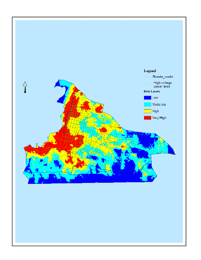
Figure 22: EOW - Natural
Breaks
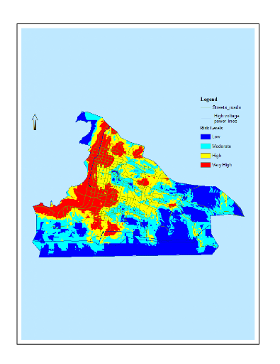
Figure 23: EOW - Geometric
Interval classification
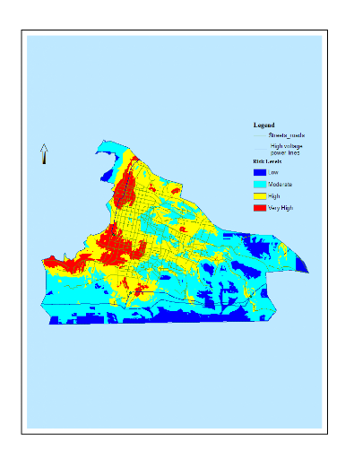
Figure 24: EOW- Equal
Interval
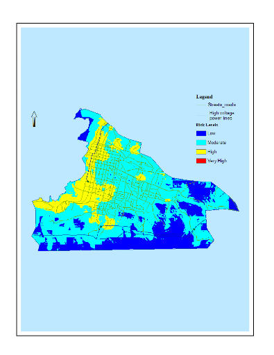
Figure 25: EOW - Defined
Interval
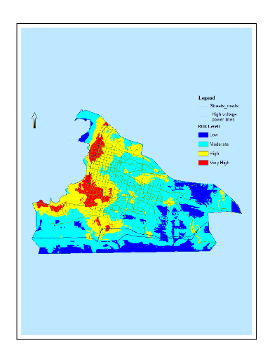
Figure 26: Equal Weight -
Quantile
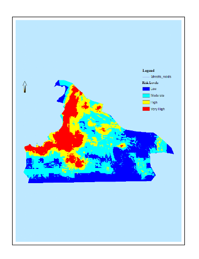
Figure 27: Equal Weight -
Natural Breaks
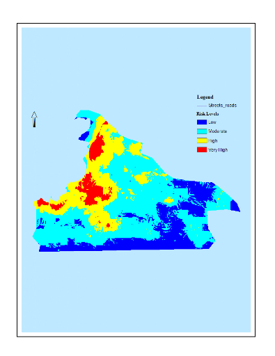
Figure 28: Equal Weight -
Equal Interval
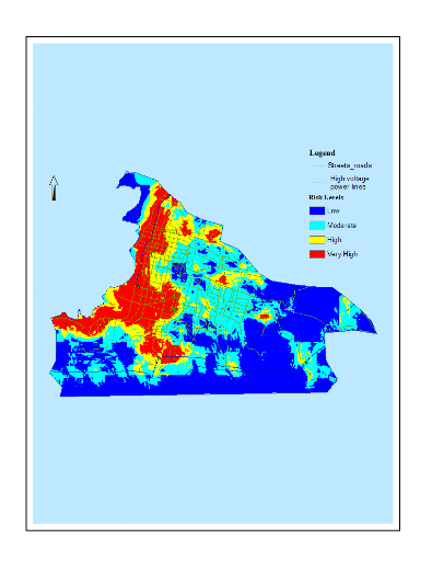
Figure 29: Equal Weight -
Geometric Interval
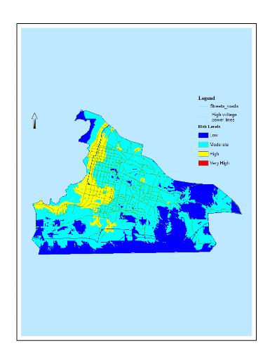
Figure 30: Equal Weight -
Defined Interval
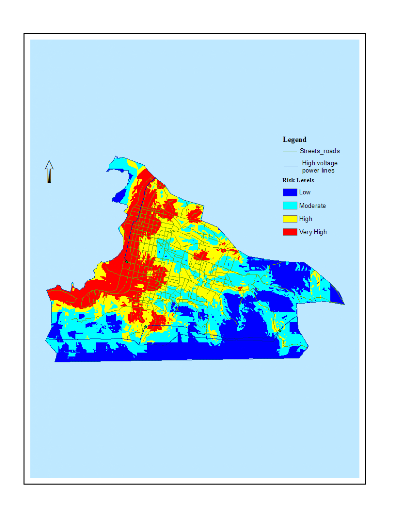
Figure 31: Own Weight -
Quantile

Figure 32: Own Weight -
Natural Breaks
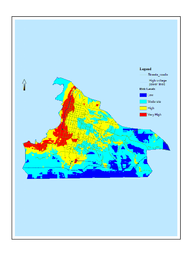
Figure 33: Own weight -
Equal interval
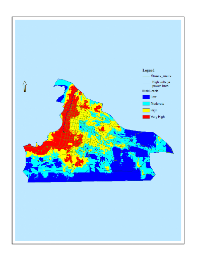
Figure 34: Own Weight -
Geometric Interval
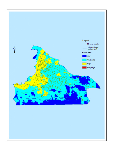
Figure 35: Own weight -
Defined
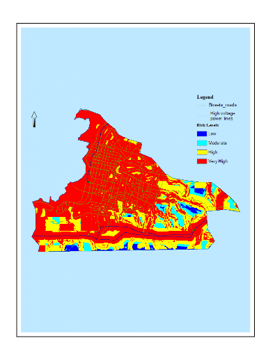
Figure 36: Maximum Output
using no classification technique

Figure 37: Maximum
Weighting - Defined
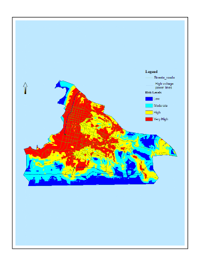
Figure 38: Traffic
Sensitivity Analysis
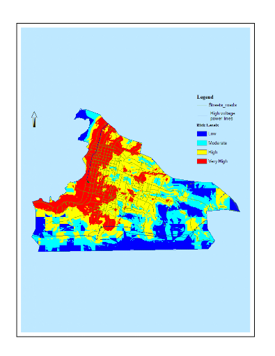
Figure 39: Waste
Sensitivity Analysis
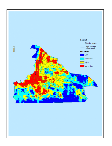
Figure 40: Proportional
Weighting Sensitivity Analysis
APPENDIX C - MODEL'S
OUTLINE
APPENDIX D - MODEL'S EXECUTION
SCRIPT
Executing (Topo to Raster): TopoToRaster "'M:\RISK Source
Data\Vector\Study_area\Rivulets.shp' # Stream;'M:\RISK Source
Data\Vector\Study_area\peaks.shp' Altitude PointElevation;'M:\RISK Source
Data\Vector\Study_area\SA_contours.shp' Elevation Contour;'M:\RISK Source
Data\Vector\Study_area\Sea_Coast_.shp' Elevation Contour" "M:\RISK Source
Data\Process\dem2" 10 "777513.9969 2048923.9338 786313.9969 2054993.9338" 20 #
# ENFORCE CONTOUR 40 # 1 0 2.5 100 "M:\RISK Source
Data\Process\synth_streams.shp" "M:\RISK Source Data\Process\sinks.shp" # #
Start Time: Sat Oct 20 16:21:37 2007
Executed (Topo to Raster) successfully.
End Time: Sat Oct 20 16:22:17 2007 (Elapsed Time: 40.00
seconds)
Executing (Buffer (5)): Buffer "M:\RISK Source
Data\Vector\Study_area\Streets_roads.shp" "M:\RISK Source
Data\Process\Streets_roads_Buf.shp" "10 Meters" FULL ROUND NONE #
Start Time: Sat Oct 20 16:22:18 2007
Executed (Buffer (5)) successfully.
End Time: Sat Oct 20 16:22:20 2007 (Elapsed Time: 2.00
seconds)
Executing (Euclidean Distance): EucDistance "M:\RISK Source
Data\Process\Streets_roads_Buf.shp" "M:\RISK Source Data\Process\Roads_eucdist"
# 10 #
Start Time: Sat Oct 20 16:22:20 2007
Executed (Euclidean Distance) successfully.
End Time: Sat Oct 20 16:22:35 2007 (Elapsed Time: 15.00
seconds)
Executing (Euclidean Distance (2)): EucDistance "M:\RISK Source
Data\Vector\Study_area\Waste_coll.shp" "M:\RISK Source
Data\Process\EucDist_Waste" # 10 #
Start Time: Sat Oct 20 16:22:36 2007
Executed (Euclidean Distance (2)) successfully.
End Time: Sat Oct 20 16:22:50 2007 (Elapsed Time: 14.00
seconds)
Executing (Euclidean Distance (4)): EucDistance "M:\RISK Source
Data\Vector\Study_area\Sea_Coast_.shp" "M:\RISK Source
Data\Process\EucDist_Sea_" # 10 #
Start Time: Sat Oct 20 16:22:51 2007
Executed (Euclidean Distance (4)) successfully.
End Time: Sat Oct 20 16:23:07 2007 (Elapsed Time: 16.00
seconds)
Executing (Buffer (3)): Buffer "M:\RISK Source
Data\Vector\Study_area\Hospitals.shp" "M:\RISK Source
Data\Process\Hosp_Buf.shp" Buffer FULL ROUND NONE #
Start Time: Sat Oct 20 16:23:08 2007
Executed (Buffer (3)) successfully.
End Time: Sat Oct 20 16:23:11 2007 (Elapsed Time: 3.00
seconds)
Executing (Euclidean Distance (5)): EucDistance "M:\RISK Source
Data\Process\Hosp_Buf.shp" "M:\RISK Source Data\Process\EucDist_Hosp" # 10 #
Start Time: Sat Oct 20 16:23:12 2007
Executed (Euclidean Distance (5)) successfully.
End Time: Sat Oct 20 16:23:26 2007 (Elapsed Time: 14.00
seconds)
Executing (Buffer (4)): Buffer "M:\RISK Source
Data\Vector\Study_area\Cemetery.shp" "M:\RISK Source
Data\Process\Cemetery_Buf.shp" "50 Meters" LEFT ROUND NONE #
Start Time: Sat Oct 20 16:23:27 2007
Executed (Buffer (4)) successfully.
End Time: Sat Oct 20 16:23:29 2007 (Elapsed Time: 2.00
seconds)
Executing (Euclidean Distance (6)): EucDistance "M:\RISK Source
Data\Process\Cemetery_Buf.shp" "M:\RISK Source Data\Process\EucDist_Cem" # 10
#
Start Time: Sat Oct 20 16:23:29 2007
Executed (Euclidean Distance (6)) successfully.
End Time: Sat Oct 20 16:23:44 2007 (Elapsed Time: 15.00
seconds)
Executing (Merge): Merge 'M:\RISK Source
Data\Vector\Study_area\Rivulets.shp';'M:\RISK Source
Data\Vector\Study_area\SA_UTSIG_rivlines.shp' "M:\RISK Source
Data\Process\streams.shp" "SHAPE_Leng SHAPE_Leng true false false 19 Double 0 0
,First,#,M:\RISK Source
Data\Vector\Study_area\Rivulets.shp,SHAPE_Leng,-1,-1,M:\RISK Source
Data\Vector\Study_area\SA_UTSIG_rivlines.shp,Shape_Leng,-1,-1;Name Name true
false false 50 Text 0 0 ,First,#,M:\RISK Source
Data\Vector\Study_area\Rivulets.shp,Name,-1,-1,M:\RISK Source
Data\Vector\Study_area\SA_UTSIG_rivlines.shp,Name,-1,-1"
Start Time: Sat Oct 20 16:23:44 2007
Executed (Merge) successfully.
End Time: Sat Oct 20 16:23:53 2007 (Elapsed Time: 9.00
seconds)
Executing (Euclidean Distance (7)): EucDistance "M:\RISK Source
Data\Process\streams.shp" "M:\RISK Source Data\Process\EucD_streams" # 10 #
Start Time: Sat Oct 20 16:23:53 2007
Executed (Euclidean Distance (7)) successfully.
End Time: Sat Oct 20 16:24:08 2007 (Elapsed Time: 15.00
seconds)
Executing (Euclidean Distance (9)): EucDistance "M:\RISK Source
Data\Vector\Study_area\SA_high voltage.shp" "M:\RISK Source
Data\Process\Pow_Line_dist" # 10 #
Start Time: Sat Oct 20 16:24:09 2007
Executed (Euclidean Distance (9)) successfully.
End Time: Sat Oct 20 16:24:25 2007 (Elapsed Time: 16.00
seconds)
Executing (Euclidean Distance (10)): EucDistance "M:\RISK Source
Data\Vector\Study_area\High_volt_pts.shp" "M:\RISK Source
Data\Process\Pow_cent_dist" # 10 #
Start Time: Sat Oct 20 16:24:25 2007
Executed (Euclidean Distance (10)) successfully.
End Time: Sat Oct 20 16:24:41 2007 (Elapsed Time: 16.00
seconds)
Executing (Euclidean Distance (8)): EucDistance "M:\RISK Source
Data\Vector\Study_area\Markets_poly.shp" "M:\RISK Source
Data\Process\EDist_Markpol" # 10 #
Start Time: Sat Oct 20 16:24:41 2007
Executed (Euclidean Distance (8)) successfully.
End Time: Sat Oct 20 16:24:57 2007 (Elapsed Time: 16.00
seconds)
Executing (Euclidean Distance (11)): EucDistance "M:\RISK Source
Data\Vector\Study_area\Markets_pts.shp" "M:\RISK Source
Data\Process\EDist_Markpts" # 10 #
Start Time: Sat Oct 20 16:24:57 2007
Executed (Euclidean Distance (11)) successfully.
End Time: Sat Oct 20 16:25:12 2007 (Elapsed Time: 15.00
seconds)
Executing (Polygon to Raster): PolygonToRaster "M:\RISK Source
Data\Vector\Study_area\pap_hab_dens_cod.shp" Dens_code "M:\RISK Source
Data\Process\pap_hab_dens.img" CELL_CENTER NONE 10
Start Time: Sat Oct 20 16:25:13 2007
Executed (Polygon to Raster) successfully.
End Time: Sat Oct 20 16:25:17 2007 (Elapsed Time: 4.00
seconds)
Executing (Single Output Map Algebra (8)): SingleOutputMapAlgebra
con(pap_hab_dens.img >= 5, 4, pap_hab_dens.img == 4, 3, pap_hab_dens.img ==
3, 2, pap_hab_dens.img <= 2, 1, 0) "M:\RISK Source
Data\Process\hab_dens_rec" 'M:\RISK Source Data\Process\pap_hab_dens.img'
Start Time: Sat Oct 20 16:25:17 2007
Executed (Single Output Map Algebra (8)) successfully.
End Time: Sat Oct 20 16:25:29 2007 (Elapsed Time: 12.00
seconds)
Executing (Single Output Map Algebra (7)): SingleOutputMapAlgebra
con(EucDist_Cem <= 50, 4, EucDist_Cem <= 150, 3, EucDist_Cem <= 250,
2, EucDist_Cem <= 350, 1, 0) "M:\RISK Source Data\Process\Cemetdist_rec"
'M:\RISK Source Data\Process\EucDist_Cem'
Start Time: Sat Oct 20 16:25:32 2007
Executed (Single Output Map Algebra (7)) successfully.
End Time: Sat Oct 20 16:25:42 2007 (Elapsed Time: 10.00
seconds)
Executing (Single Output Map Algebra (6)): SingleOutputMapAlgebra
"con(EucDist_Hosp <= 50, 4, EucDist_Hosp <= 100, 3, EucDist_Hosp <=
200, 2, EucDist_Hosp <= 300, 1, 0) " "M:\RISK Source
Data\Process\HospDist_rec" 'M:\RISK Source Data\Process\EucDist_Hosp'
Start Time: Sat Oct 20 16:25:46 2007
Executed (Single Output Map Algebra (6)) successfully.
End Time: Sat Oct 20 16:25:54 2007 (Elapsed Time: 8.00
seconds)
Executing (Single Output Map Algebra (24)):
SingleOutputMapAlgebra con(EDist_Markpol <= 100, 4, EDist_Markpol <= 200,
3, EDist_Markpol <= 300, 2, EDist_Markpol <= 400, 1, 0) "M:\RISK Source
Data\Process\mkpoldist_rec" 'M:\RISK Source Data\Process\EDist_Markpol'
Start Time: Sat Oct 20 16:25:58 2007
Executed (Single Output Map Algebra (24)) successfully.
End Time: Sat Oct 20 16:26:07 2007 (Elapsed Time: 9.00
seconds)
Executing (Single Output Map Algebra (25)):
SingleOutputMapAlgebra "con(EDist_Markpts <= 100, 4, EDist_Markpts <=
200, 3, EDist_Markpts <= 300, 2, EDist_Markpts <= 400, 1, 0) " "M:\RISK
Source Data\Process\mkptsdist_rec" 'M:\RISK Source
Data\Process\EDist_Markpts'
Start Time: Sat Oct 20 16:26:07 2007
Executed (Single Output Map Algebra (25)) successfully.
End Time: Sat Oct 20 16:26:16 2007 (Elapsed Time: 9.00
seconds)
Executing (Single Output Map Algebra (5)): SingleOutputMapAlgebra
max(mkpoldist_rec, mkptsdist_rec) "M:\RISK Source Data\Process\markets_pol"
'M:\RISK Source Data\Process\mkpoldist_rec';'M:\RISK Source
Data\Process\mkptsdist_rec'
Start Time: Sat Oct 20 16:26:17 2007
Executed (Single Output Map Algebra (5)) successfully.
End Time: Sat Oct 20 16:26:28 2007 (Elapsed Time: 11.00
seconds)
Executing (Single Output Map Algebra (12)):
SingleOutputMapAlgebra con(Pow_cent_dist <= 300, 4, Pow_cent_dist <= 500,
3, Pow_cent_dist <= 700, 2, Pow_cent_dist <= 1000, 1, 0) "M:\RISK Source
Data\Process\Pow_cent_rec" 'M:\RISK Source Data\Process\Pow_cent_dist'
Start Time: Sat Oct 20 16:26:32 2007
Executed (Single Output Map Algebra (12)) successfully.
End Time: Sat Oct 20 16:26:41 2007 (Elapsed Time: 9.00
seconds)
Executing (Single Output Map Algebra (19)):
SingleOutputMapAlgebra con(Pow_Line_dist <= 150, 4, Pow_Line_dist <= 300,
3, Pow_Line_dist <= 400, 2, Pow_Line_dist <= 500, 1, 0)
"M:\RISK Source Data\Process\Pow_Line_rec" 'M:\RISK Source
Data\Process\Pow_Line_dist'
Start Time: Sat Oct 20 16:26:42 2007
Executed (Single Output Map Algebra (19)) successfully.
End Time: Sat Oct 20 16:26:51 2007 (Elapsed Time: 9.00
seconds)
Executing (Single Output Map Algebra (20)):
SingleOutputMapAlgebra max(Pow_cent_rec,Pow_Line_rec) "M:\RISK Source
Data\Process\Power_factor" 'M:\RISK Source Data\Process\Pow_cent_rec';'M:\RISK
Source Data\Process\Pow_Line_rec'
Start Time: Sat Oct 20 16:26:51 2007
Executed (Single Output Map Algebra (20)) successfully.
End Time: Sat Oct 20 16:27:01 2007 (Elapsed Time: 10.00
seconds)
Executing (Single Output Map Algebra (21)):
SingleOutputMapAlgebra con(EucDist_Sea_ <= 300, 4, EucDist_Sea_ <= 500,
3, EucDist_Sea_ <= 700, 2, EucDist_Sea_ <= 1000, 1, 0) "M:\RISK Source
Data\Process\sea_dist_rec_" 'M:\RISK Source Data\Process\EucDist_Sea_'
Start Time: Sat Oct 20 16:27:06 2007
Executed (Single Output Map Algebra (21)) successfully.
End Time: Sat Oct 20 16:27:15 2007 (Elapsed Time: 9.00
seconds)
Executing (Single Output Map Algebra (9)): SingleOutputMapAlgebra
con(EucD_streams <= 100, 4, EucD_streams <= 200, 3, EucD_streams <=
300, 2, EucD_streams <= 400, 1) "M:\RISK Source Data\Process\Str_dist_rec"
'M:\RISK Source Data\Process\EucD_streams'
Start Time: Sat Oct 20 16:27:19 2007
Executed (Single Output Map Algebra (9)) successfully.
End Time: Sat Oct 20 16:27:29 2007 (Elapsed Time: 10.00
seconds)
Executing (Fill): Fill "M:\RISK Source Data\Process\dem2"
"M:\RISK Source Data\Process\dem_fill" #
Start Time: Sat Oct 20 16:27:30 2007
Executed (Fill) successfully.
End Time: Sat Oct 20 16:31:45 2007 (Elapsed Time: 4 minutes 15
seconds)
Executing (Extract by Mask): ExtractByMask "M:\RISK Source
Data\Process\dem_fill" "M:\RISK Source Data\Vector\Study_area\sa_mask" "M:\RISK
Source Data\Process\pap_dem"
Start Time: Sat Oct 20 16:31:46 2007
Executed (Extract by Mask) successfully.
End Time: Sat Oct 20 16:32:00 2007 (Elapsed Time: 14.00
seconds)
Executing (Slope): Slope "M:\RISK Source Data\Process\pap_dem"
"M:\RISK Source Data\Process\PAP_Slope" PERCENT_RISE 1
Start Time: Sat Oct 20 16:32:02 2007
Executed (Slope) successfully.
End Time: Sat Oct 20 16:32:17 2007 (Elapsed Time: 15.00
seconds)
Executing (Single Output Map Algebra (23)):
SingleOutputMapAlgebra con(PAP_Slope <= 5, 4, PAP_Slope <= 15, 3,
PAP_Slope <= 25, 2, PAP_Slope > 25, 1, 0) "M:\RISK Source
Data\Process\pap_slop_rec" 'M:\RISK Source Data\Process\PAP_Slope'
Start Time: Sat Oct 20 16:32:18 2007
Executed (Single Output Map Algebra (23)) successfully.
End Time: Sat Oct 20 16:32:31 2007 (Elapsed Time: 13.00
seconds)
Executing (Single Output Map Algebra (10)):
SingleOutputMapAlgebra "0.7*(Streams distance reclassified) + 0.3*pap_slop_rec"
"M:\RISK Source Data\Process\Streams_pol" 'M:\RISK Source
Data\Process\Str_dist_rec';'M:\RISK Source Data\Process\pap_slop_rec'
Start Time: Sat Oct 20 16:32:33 2007
Executed (Single Output Map Algebra (10)) successfully.
End Time: Sat Oct 20 16:32:47 2007 (Elapsed Time: 14.00
seconds)
Executing (Reclassify): Reclassify "M:\RISK Source
Data\Process\Streams_pol" VALUE "1 2.4100469267072113 1;2.4100469267072113
3.0567306046542977 2;3.0567306046542977 3.3533163220529132 3;3.3533163220529132
4 4;NODATA 0" "M:\RISK Source Data\Process\str_pol_rec1" DATA
Start Time: Sat Oct 20 16:32:49 2007
Executed (Reclassify) successfully.
End Time: Sat Oct 20 16:33:27 2007 (Elapsed Time: 38.00
seconds)
Executing (Feature to Raster (2)): FeatureToRaster "M:\RISK
Source Data\Vector\Study_area\Land_use.shp" L_U_Code "M:\RISK Source
Data\Process\land_use" 10
Start Time: Sat Oct 20 16:33:33 2007
Executed (Feature to Raster (2)) successfully.
End Time: Sat Oct 20 16:33:41 2007 (Elapsed Time: 8.00
seconds)
Executing (Single Output Map Algebra (18)):
SingleOutputMapAlgebra con(Roads_eucdist <= 50, 4, Roads_eucdist <= 100,
3, Roads_eucdist <= 200, 2, Roads_eucdist <= 300, 1) "M:\RISK Source
Data\Process\roadist_rec" 'M:\RISK Source Data\Process\Roads_eucdist'
Start Time: Sat Oct 20 16:33:41 2007
Executed (Single Output Map Algebra (18)) successfully.
End Time: Sat Oct 20 16:33:55 2007 (Elapsed Time: 14.00
seconds)
Executing (IDW): Idw "M:\RISK Source
Data\Vector\Study_area\pap_elevs.shp" PAP_DEM "M:\RISK Source
Data\Process\Elev_4_40" 10 4 "VARIABLE 12 50" #
Start Time: Sat Oct 20 16:33:56 2007
Executed (IDW) successfully.
End Time: Sat Oct 20 16:34:19 2007 (Elapsed Time: 23.00
seconds)
Executing (Reclassify (7)): Reclassify "M:\RISK Source
Data\Process\Elev_4_40" Value "-2 100 4;100 300 3;300 500 2;500 600 1;NODATA 0"
"M:\RISK Source Data\Process\elev_reclass" DATA
Start Time: Sat Oct 20 16:34:20 2007
Executed (Reclassify (7)) successfully.
End Time: Sat Oct 20 16:34:53 2007 (Elapsed Time: 33.00
seconds)
Executing (Polygon to Raster (2)): PolygonToRaster "M:\RISK
Source Data\Vector\Study_area\Streets_roads_Buffer.shp" Traf_dens "M:\RISK
Source Data\Process\traf_buf_den" CELL_CENTER NONE 10
Start Time: Sat Oct 20 16:34:54 2007
Executed (Polygon to Raster (2)) successfully.
End Time: Sat Oct 20 16:35:08 2007 (Elapsed Time: 14.00
seconds)
Executing (Single Output Map Algebra): SingleOutputMapAlgebra
"0.35*(1.00*roadist_rec) + 0.15*(1.00*Land_Use) + 0.15*(1.00*elev_reclass) +
0.35*(1.00*traf_buf_den)" "M:\RISK Source Data\Process\traf_pol_risk" 'M:\RISK
Source Data\Process\land_use';'M:\RISK Source
Data\Process\roadist_rec';'M:\RISK Source Data\Process\elev_reclass';'M:\RISK
Source Data\Process\traf_buf_den'
Start Time: Sat Oct 20 16:35:14 2007
Executed (Single Output Map Algebra) successfully.
End Time: Sat Oct 20 16:35:33 2007 (Elapsed Time: 19.00
seconds)
Executing (Reclassify (2)): Reclassify "M:\RISK Source
Data\Process\traf_pol_risk" VALUE "0.94999998807907104 2.1672228247818373
1;2.1672228247818373 2.8767925732977973 2;2.8767925732977973 3.2904302514840391
3;3.2904302514840391 4 4;NODATA 0" "M:\RISK Source Data\Process\traf_pol_fin1"
DATA
Start Time: Sat Oct 20 16:35:41 2007
Executed (Reclassify (2)) successfully.
End Time: Sat Oct 20 16:36:15 2007 (Elapsed Time: 34.00
seconds)
Executing (Feature to Raster (5)): FeatureToRaster "M:\RISK
Source Data\Vector\Study_area\Waste_coll_Buf.shp" Net_cond "M:\RISK Source
Data\Process\Wastecond_ras" 10
Start Time: Sat Oct 20 16:36:23 2007
Executed (Feature to Raster (5)) successfully.
End Time: Sat Oct 20 16:36:32 2007 (Elapsed Time: 9.00
seconds)
Executing (Reclassify (21)): Reclassify "M:\RISK Source
Data\Process\Wastecond_ras" VALUE "1 1;1 2 2;2 3 3;3 4 4;NODATA 0" "M:\RISK
Source Data\Process\waste_condrec" DATA
Start Time: Sat Oct 20 16:36:38 2007
Executed (Reclassify (21)) successfully.
End Time: Sat Oct 20 16:37:14 2007 (Elapsed Time: 36.00
seconds)
Executing (Euclidean Distance (3)): EucDistance "M:\RISK Source
Data\Vector\Study_area\Waste_coll.shp" "M:\RISK Source
Data\Process\Waste_Edist" # 10 #
Start Time: Sat Oct 20 16:37:14 2007
Executed (Euclidean Distance (3)) successfully.
End Time: Sat Oct 20 16:37:39 2007 (Elapsed Time: 25.00
seconds)
Executing (Single Output Map Algebra (11)):
SingleOutputMapAlgebra con(Waste_Edist > 400, 1, 0) "M:\RISK Source
Data\Process\WasteDist_400" 'M:\RISK Source Data\Process\Waste_Edist'
Start Time: Sat Oct 20 16:37:41 2007
Executed (Single Output Map Algebra (11)) successfully.
End Time: Sat Oct 20 16:37:55 2007 (Elapsed Time: 14.00
seconds)
Executing (Single Output Map Algebra (14)):
SingleOutputMapAlgebra con(WasteDist_400 == 1 & pap_hab_dens.img == 1, 1,
WasteDist_400 == 1 & pap_hab_dens.img == 2, 2, WasteDist_400 == 1 &
pap_hab_dens.img == 3, 3, WasteDist_400 == 1 & pap_hab_dens.img == 4, 4, 0)
"M:\RISK Source Data\Process\WastD400_hden" 'M:\RISK Source
Data\Process\WasteDist_400';'M:\RISK Source Data\Process\pap_hab_dens.img'
Start Time: Sat Oct 20 16:38:04 2007
Executed (Single Output Map Algebra (14)) successfully.
End Time: Sat Oct 20 16:38:28 2007 (Elapsed Time: 24.00
seconds)
Executing (Single Output Map Algebra (2)): SingleOutputMapAlgebra
con(EucDist_Waste <= 100, 4, EucDist_Waste <= 200, 3, EucDist_Waste <=
300, 2, EucDist_Waste <= 400, 1, 0) "M:\RISK Source Data\Process\Waste_dist"
'M:\RISK Source Data\Process\EucDist_Waste'
Start Time: Sat Oct 20 16:38:38 2007
Executed (Single Output Map Algebra (2)) successfully.
End Time: Sat Oct 20 16:38:54 2007 (Elapsed Time: 16.00
seconds)
Executing (Single Output Map Algebra (22)):
SingleOutputMapAlgebra "WastD400_hden + Waste_dist" "M:\RISK Source
Data\Process\Wastdist_sum" 'M:\RISK Source Data\Process\WastD400_hden';'M:\RISK
Source Data\Process\Waste_dist'
Start Time: Sat Oct 20 16:39:05 2007
Executed (Single Output Map Algebra (22)) successfully.
End Time: Sat Oct 20 16:39:21 2007 (Elapsed Time: 16.00
seconds)
Executing (Single Output Map Algebra (13)):
SingleOutputMapAlgebra con(Wastdist_sum > 0, Wastdist_sum) "M:\RISK Source
Data\Process\Waste_sum_rec" 'M:\RISK Source Data\Process\Wastdist_sum'
Start Time: Sat Oct 20 16:39:30 2007
Executed (Single Output Map Algebra (13)) successfully.
End Time: Sat Oct 20 16:39:51 2007 (Elapsed Time: 21.00
seconds)
Executing (Single Output Map Algebra (3)): SingleOutputMapAlgebra
"0.5*(1.0*Waste_sum_rec) + 0.3*(1.0*waste_condrec) + 0.2*(1.0*elev_reclass)"
"M:\RISK Source Data\Process\Waste_factor" 'M:\RISK Source
Data\Process\elev_reclass';'M:\RISK Source Data\Process\waste_condrec';'M:\RISK
Source Data\Process\Waste_sum_rec'
Start Time: Sat Oct 20 16:39:52 2007
Executed (Single Output Map Algebra (3)) successfully.
End Time: Sat Oct 20 16:40:12 2007 (Elapsed Time: 20.00
seconds)
Executing (Reclassify (3)): Reclassify "M:\RISK Source
Data\Process\Waste_factor" VALUE "0.69999998807907104 1.9015878793008327
1;1.9015878793008327 2.6912910404759467 2;2.6912910404759467 3.210296838824886
3;3.210296838824886 4 4;NODATA 0" "M:\RISK Source Data\Process\waste_risks1"
DATA
Start Time: Sat Oct 20 16:40:22 2007
Executed (Reclassify (3)) successfully.
End Time: Sat Oct 20 16:40:56 2007 (Elapsed Time: 34.00
seconds)
Executing (Single Output Map Algebra (15)):
SingleOutputMapAlgebra "0.13 * (1.00*traf_pol_fin1) + 0.14 *
(1.00*Waste_Risks1) + 0.08 * (1.00*Cemetdist_rec) + 0.08 * (1.00*HospDist_rec)
+ 0.13 * (1.00*markets_pol) + 0.13 * (1.00*hab_dens_rec) + 0.12 *
(1.00*Str_pol_rec1) + 0.11 * (1.00*Sea_dist_rec_) + 0.08 * (1.00*power_factor)"
"M:\RISK Source Data\Process\EOW_output" 'M:\RISK Source
Data\Process\hab_dens_rec';'M:\RISK Source Data\Process\Cemetdist_rec';'M:\RISK
Source Data\Process\HospDist_rec';'M:\RISK Source
Data\Process\markets_pol';'M:\RISK Source Data\Process\Power_factor';'M:\RISK
Source Data\Process\sea_dist_rec_';'M:\RISK Source
Data\Process\str_pol_rec1';'M:\RISK Source Data\Process\traf_pol_fin1';'M:\RISK
Source Data\Process\waste_risks1'
Start Time: Sat Oct 20 16:41:06 2007
Executed (Single Output Map Algebra (15)) successfully.
End Time: Sat Oct 20 16:41:24 2007 (Elapsed Time: 18.00
seconds)
Executing (Reclassify (4)): Reclassify "M:\RISK Source
Data\Process\EOW_output" VALUE "0.12999999523162842 1.0815625195391476
1;1.0815625195391476 1.5300000309944153 2;1.5300000309944153 1.9346875413320959
3;1.9346875413320959 2.9300000667572021 4" "M:\RISK Source
Data\Process\EOW_Rec_Quant" DATA
Start Time: Sat Oct 20 16:41:35 2007
Executed (Reclassify (4)) successfully.
End Time: Sat Oct 20 16:42:08 2007 (Elapsed Time: 33.00
seconds)
Executing (Single Output Map Algebra (17)):
SingleOutputMapAlgebra "0.14*(1.00*traf_pol_fin1) + 0.16*(1.00*Waste_Risks1) +
0.06*(1.00*Cemetdist_rec) + 0.06*(1.00*HospDist_rec) + 0.10*(1.00*markets_pol)
+ 0.14*(1.00*hab_dens_rec) + 0.10*(1.00*Str_pol_rec1) +
0.16*(1.00*Sea_dist_rec_) + 0.08*(1.00*power_factor)" "M:\RISK Source
Data\Process\Own_rank_out" 'M:\RISK Source Data\Process\hab_dens_rec';'M:\RISK
Source Data\Process\Cemetdist_rec';'M:\RISK Source
Data\Process\HospDist_rec';'M:\RISK Source Data\Process\markets_pol';'M:\RISK
Source Data\Process\Power_factor';'M:\RISK Source
Data\Process\sea_dist_rec_';'M:\RISK Source Data\Process\str_pol_rec1';'M:\RISK
Source Data\Process\traf_pol_fin1';'M:\RISK Source
Data\Process\waste_risks1'
Start Time: Sat Oct 20 16:42:19 2007
Executed (Single Output Map Algebra (17)) successfully.
End Time: Sat Oct 20 16:42:38 2007 (Elapsed Time: 19.00
seconds)
Executing (Reclassify (6)): Reclassify "M:\RISK Source
Data\Process\Own_rank_out" VALUE "0.14000000059604645 1.0996874694828875
1;1.0996874694828875 1.5737499541137367 2;1.5737499541137367 2.013124939869158
3;2.013124939869158 3.0999999046325684 4" "M:\RISK Source
Data\Process\OwnWght_quan" DATA
Start Time: Sat Oct 20 16:42:49 2007
Executed (Reclassify (6)) successfully.
End Time: Sat Oct 20 16:43:05 2007 (Elapsed Time: 16.00
seconds)
Executing (Reclassify (8)): Reclassify "M:\RISK Source
Data\Process\EOW_output" VALUE "0.12999999523162842 0.83000001311302185
1;0.83000001311302185 1.5300000309944153 2;1.5300000309944153
2.2300000488758087 3;2.2300000488758087 2.9300000667572021 4" "M:\RISK Source
Data\Process\EOWrec_EqInt" DATA
Start Time: Sat Oct 20 16:43:16 2007
Executed (Reclassify (8)) successfully.
End Time: Sat Oct 20 16:43:49 2007 (Elapsed Time: 33.00
seconds)
Executing (Reclassify (9)): Reclassify "M:\RISK Source
Data\Process\EOW_output" VALUE "0.12999999523162842 0.99406251730397344
1;0.99406251730397344 1.497187530156225 2;1.497187530156225 2.0550000444054604
3;2.0550000444054604 2.9300000667572021 4" "M:\RISK Source
Data\Process\EOWrec_Jenks" DATA
Start Time: Sat Oct 20 16:44:01 2007
Executed (Reclassify (9)) successfully.
End Time: Sat Oct 20 16:44:16 2007 (Elapsed Time: 15.00
seconds)
Executing (Reclassify (10)): Reclassify "M:\RISK Source
Data\Process\EOW_output" VALUE "0.12999999523162842 1.107699205033057
1;1.107699205033057 1.5300000309944153 2;1.5300000309944153 1.9523008569557736
3;1.9523008569557736 2.9300000667572021 4" "M:\RISK Source
Data\Process\EOWrec_GeoInt" DATA
Start Time: Sat Oct 20 16:44:28 2007
Executed (Reclassify (10)) successfully.
End Time: Sat Oct 20 16:44:47 2007 (Elapsed Time: 19.00
seconds)
Executing (Single Output Map Algebra (4)): SingleOutputMapAlgebra
max(sea_dist_rec_,str_pol_rec1,waste_risks1,markets_pol,traf_pol_fin1,Power_factor,Cemetdist_rec,hab_dens_rec,HospDist_rec)
"M:\RISK Source Data\Process\Max_risks_out" 'M:\RISK Source
Data\Process\sea_dist_rec_';'M:\RISK Source Data\Process\str_pol_rec1';'M:\RISK
Source Data\Process\waste_risks1';'M:\RISK Source
Data\Process\markets_pol';'M:\RISK Source Data\Process\traf_pol_fin1';'M:\RISK
Source Data\Process\Power_factor';'M:\RISK Source
Data\Process\Cemetdist_rec';'M:\RISK Source Data\Process\hab_dens_rec';'M:\RISK
Source Data\Process\HospDist_rec'
Start Time: Sat Oct 20 16:45:00 2007
Executed (Single Output Map Algebra (4)) successfully.
End Time: Sat Oct 20 16:45:47 2007 (Elapsed Time: 47.00
seconds)
Executing (Reclassify (14)): Reclassify "M:\RISK Source
Data\Process\Max_risks_out" VALUE "1 1.99609375 1;1.99609375 2.9921875
2;2.9921875 4 3" "M:\RISK Source Data\Process\MaxRisk_quant" DATA
Start Time: Sat Oct 20 16:46:02 2007
Executed (Reclassify (14)) successfully.
End Time: Sat Oct 20 16:46:26 2007 (Elapsed Time: 24.00
seconds)
Executing (Reclassify (15)): Reclassify "M:\RISK Source
Data\Process\Own_rank_out" VALUE "0.14000000059604645 0.87999997660517693
1;0.87999997660517693 1.6199999526143074 2;1.6199999526143074
2.3599999286234379 3;2.3599999286234379 3.0999999046325684 4" "M:\RISK Source
Data\Process\OwnWght_EqInt" DATA
Start Time: Sat Oct 20 16:46:39 2007
Executed (Reclassify (15)) successfully.
End Time: Sat Oct 20 16:47:03 2007 (Elapsed Time: 24.00
seconds)
Executing (Reclassify (16)): Reclassify "M:\RISK Source
Data\Process\Own_rank_out" VALUE "0.14000000059604645 0.97249997360631824
1;0.97249997360631824 1.5506249548634514 2;1.5506249548634514
2.1749999346211553 3;2.1749999346211553 3.0999999046325684 4" "M:\RISK Source
Data\Process\OwnWght_Jenks" DATA
Start Time: Sat Oct 20 16:47:17 2007
Executed (Reclassify (16)) successfully.
End Time: Sat Oct 20 16:47:40 2007 (Elapsed Time: 23.00
seconds)
Executing (Reclassify (17)): Reclassify "M:\RISK Source
Data\Process\Own_rank_out" VALUE "0.14000000059604645 1.154653732663663
1;1.154653732663663 1.6199999526143072 2;1.6199999526143072 2.0853461725649516
3;2.0853461725649516 3.0999999046325684 4" "M:\RISK Source
Data\Process\OwnWght_GeoIn" DATA
Start Time: Sat Oct 20 16:47:54 2007
Executed (Reclassify (17)) successfully.
End Time: Sat Oct 20 16:48:18 2007 (Elapsed Time: 24.00
seconds)
Executing (Reclassify (18)): Reclassify "M:\RISK Source
Data\Process\Max_risks_out" VALUE "1 1.75 1;1.75 2.5 2;2.5 3.25 3;3.25 4 4"
"M:\RISK Source Data\Process\MaxRisk_EqInt" DATA
Start Time: Sat Oct 20 16:48:32 2007
Executed (Reclassify (18)) successfully.
End Time: Sat Oct 20 16:48:56 2007 (Elapsed Time: 24.00
seconds)
Executing (Reclassify (19)): Reclassify "M:\RISK Source
Data\Process\Max_risks_out" VALUE "1 1;1 1.99609375 2;1.99609375 2.9921875
3;2.9921875 4 4" "M:\RISK Source Data\Process\MaxRisk_Jenks" DATA
Start Time: Sat Oct 20 16:49:10 2007
Executed (Reclassify (19)) successfully.
End Time: Sat Oct 20 16:49:53 2007 (Elapsed Time: 43.00
seconds)
Executing (Reclassify (20)): Reclassify "M:\RISK Source
Data\Process\Max_risks_out" VALUE "1 1.75 1;1.75 2.5 2;2.5 3.25 3;3.25 4 4"
"M:\RISK Source Data\Process\MaxRisk_geoIn" DATA
Start Time: Sat Oct 20 16:50:07 2007
Executed (Reclassify (20)) successfully.
End Time: Sat Oct 20 16:50:31 2007 (Elapsed Time: 24.00
seconds)
Executing (Weighted Overlay): WeightedOverlay "('M:\RISK Source
Data\Process\HospDist_rec' 11 'VALUE' (0 Restricted; 1 1; 2 2; 3 3; 4 4;NODATA
NODATA); 'M:\RISK Source Data\Process\Cemetdist_rec' 11 'VALUE' (0 Restricted;
1 1; 2 2; 3 3; 4 4;NODATA NODATA); 'M:\RISK Source Data\Process\str_pol_rec1'
11 'VALUE' (0 Restricted; 1 1; 2 2; 3 3; 4 4;NODATA NODATA); 'M:\RISK Source
Data\Process\Power_factor' 11 'VALUE' (0 Restricted; 1 1; 2 2; 3 3; 4 4;NODATA
NODATA); 'M:\RISK Source Data\Process\sea_dist_rec_' 11 'VALUE' (0 Restricted;
1 1; 2 2; 3 3; 4 4;NODATA NODATA); 'M:\RISK Source Data\Process\markets_pol' 11
'VALUE' (0 Restricted; 1 1; 2 2; 3 3; 4 4;NODATA NODATA); 'M:\RISK Source
Data\Process\traf_pol_fin1' 11 'VALUE' (1 1; 2 2; 3 3; 4 4;NODATA NODATA);
'M:\RISK Source Data\Process\waste_risks1' 11 'VALUE' (1 1; 2 2; 3 3; 4
4;NODATA NODATA); 'M:\RISK Source Data\Process\hab_dens_rec' 12 'VALUE' (1 1; 2
2; 3 3; 4 4;NODATA NODATA));1 4 1" "M:\RISK Source
Data\Process\Equal_influ1"
Start Time: Sat Oct 20 16:50:45 2007
Executed (Weighted Overlay) successfully.
End Time: Sat Oct 20 16:54:42 2007 (Elapsed Time: 3 minutes 57
seconds)
Executing (Single Output Map Algebra (27)):
SingleOutputMapAlgebra con(waste_risks1 >= 2 & hab_dens_rec >= 2
& traf_pol_fin1 >=2 & markets_pol >= 2 & sea_dist_rec_
>= 2 & Power_factor >= 2 & str_pol_rec1 >= 2 &
Cemetdist_rec >= 2 & HospDist_rec >= 2, 1, 0) "M:\RISK Source
Data\Process\Highrisk_Int" 'M:\RISK Source Data\Process\waste_risks1';'M:\RISK
Source Data\Process\hab_dens_rec';'M:\RISK Source
Data\Process\traf_pol_fin1';'M:\RISK Source Data\Process\markets_pol';'M:\RISK
Source Data\Process\sea_dist_rec_';'M:\RISK Source
Data\Process\Power_factor';'M:\RISK Source Data\Process\str_pol_rec1';'M:\RISK
Source Data\Process\Cemetdist_rec';'M:\RISK Source
Data\Process\HospDist_rec'
Start Time: Sat Oct 20 16:55:14 2007
Executed (Single Output Map Algebra (27)) successfully.
End Time: Sat Oct 20 16:56:32 2007 (Elapsed Time: 1 minutes 18
seconds)
Executing (Single Output Map Algebra (16)):
SingleOutputMapAlgebra "0.12*traf_pol_fin1 + 0.11*Waste_Risks1 +
0.11*Cemetdist_rec + 0.11*HospDist_rec + 0.11*markets_pol + 0.11*hab_dens_rec +
0.11*Str_pol_rec1 + 0.11*Sea_dist_rec_ + 0.11*power_factor" "M:\RISK Source
Data\Process\Equalweight" 'M:\RISK Source Data\Process\hab_dens_rec';'M:\RISK
Source Data\Process\Cemetdist_rec';'M:\RISK Source
Data\Process\HospDist_rec';'M:\RISK Source Data\Process\markets_pol';'M:\RISK
Source Data\Process\Power_factor';'M:\RISK Source
Data\Process\sea_dist_rec_';'M:\RISK Source Data\Process\str_pol_rec1';'M:\RISK
Source Data\Process\traf_pol_fin1';'M:\RISK Source
Data\Process\waste_risks1'
Start Time: Sat Oct 20 16:57:00 2007
Executed (Single Output Map Algebra (16)) successfully.
End Time: Sat Oct 20 16:58:06 2007 (Elapsed Time: 1 minutes 6
seconds)
Executing (Reclassify (5)): Reclassify "M:\RISK Source
Data\Process\Equalweight" VALUE "0.10000000000000001 0.98991839663358405
1;0.98991839663358405 1.3262563003227115 2;1.3262563003227115
1.7710903019760735 3;1.7710903019760735 3 4" "M:\RISK Source
Data\Process\Quan_Eqweight" DATA
Start Time: Sat Oct 20 16:58:23 2007
Executed (Reclassify (5)) successfully.
End Time: Sat Oct 20 16:59:39 2007 (Elapsed Time: 1 minutes 16
seconds)
Executing (Reclassify (12)): Reclassify "M:\RISK Source
Data\Process\Equalweight" VALUE "0.10000000000000001 1.1316237692284663
1;1.1316237692284663 1.4998500570654871 2;1.4998500570654871 1.868076344902508
3;1.868076344902508 3 4" "M:\RISK Source Data\Process\GeoIn_eqWeigh" DATA
Start Time: Sat Oct 20 17:00:00 2007
Executed (Reclassify (12)) successfully.
End Time: Sat Oct 20 17:00:57 2007 (Elapsed Time: 57.00
seconds)
Executing (Reclassify (13)): Reclassify "M:\RISK Source
Data\Process\Equalweight" VALUE "0.10000000000000001 0.98991839663358405
1;0.98991839663358405 1.4347523982869461 2;1.4347523982869461
1.8795863999403082 3;1.8795863999403082 3 4" "M:\RISK Source
Data\Process\Jenks_EqWeigh" DATA
Start Time: Sat Oct 20 17:01:14 2007
Executed (Reclassify (13)) successfully.
End Time: Sat Oct 20 17:02:12 2007 (Elapsed Time: 58.00
seconds)
Executing (Reclassify (11)): Reclassify "M:\RISK Source
Data\Process\Equalweight" VALUE "0.10000000000000001 0.80547503009438515
1;0.80547503009438515 1.4998500570654869 2;1.4998500570654869
2.1942250840365887 3;2.1942250840365887 3 4" "M:\RISK Source
Data\Process\EqInt_Eqweigh" DATA
Start Time: Sat Oct 20 17:02:28 2007
Executed (Reclassify (11)) successfully.
End Time: Sat Oct 20 17:03:27 2007 (Elapsed Time: 59.00
seconds)
Executing (Reclassify (22)): Reclassify "M:\RISK Source
Data\Process\EOW_output" VALUE "0 1 1;1 2 2;2 3 3;3 4 4" "M:\RISK Source
Data\Process\EOW_defined" DATA
Start Time: Sat Oct 20 17:03:44 2007
Executed (Reclassify (22)) successfully.
End Time: Sat Oct 20 17:04:41 2007 (Elapsed Time: 57.00
seconds)
Executing (Reclassify (23)): Reclassify "M:\RISK Source
Data\Process\Own_rank_out" VALUE "0 1 1;1 2 2;2 3 3;3 4 4" "M:\RISK Source
Data\Process\Own_defined" DATA
Start Time: Sat Oct 20 17:04:59 2007
Executed (Reclassify (23)) successfully.
End Time: Sat Oct 20 17:05:57 2007 (Elapsed Time: 58.00
seconds)
Executing (Reclassify (25)): Reclassify "M:\RISK Source
Data\Process\Max_risks_out" VALUE "0 1 1;1 2 2;2 3 3;3 4 4" "M:\RISK Source
Data\Process\Max_defined" DATA
Start Time: Sat Oct 20 17:06:15 2007
Executed (Reclassify (25)) successfully.
End Time: Sat Oct 20 17:07:14 2007 (Elapsed Time: 59.00
seconds)
Executing (Reclassify (26)): Reclassify "M:\RISK Source
Data\Process\Equalweight" VALUE "0 1 1;1 2 2;2 3 3;3 4 4" "M:\RISK Source
Data\Process\EqWgh_defined" DATA
Start Time: Sat Oct 20 17:07:32 2007
Executed (Reclassify (26)) successfully.
End Time: Sat Oct 20 17:08:29 2007 (Elapsed Time: 57.00
seconds)
Executing (Single Output Map Algebra (30)):
SingleOutputMapAlgebra "0.10*traf_pol_fin1 + 0.30*Waste_Risks1 +
0.05*Cemetdist_rec + 0.05*HospDist_rec + 0.10*markets_pol + 0.10*hab_dens_rec +
0.10*Str_pol_rec1 + 0.10*Sea_dist_rec_ + 0.10*power_factor" "M:\RISK Source
Data\Process\Sens_An_Waste" 'M:\RISK Source Data\Process\hab_dens_rec';'M:\RISK
Source Data\Process\waste_risks1';'M:\RISK Source
Data\Process\traf_pol_fin1';'M:\RISK Source Data\Process\markets_pol';'M:\RISK
Source Data\Process\Cemetdist_rec';'M:\RISK Source
Data\Process\Power_factor';'M:\RISK Source Data\Process\str_pol_rec1';'M:\RISK
Source Data\Process\HospDist_rec';'M:\RISK Source
Data\Process\sea_dist_rec_'
Start Time: Sat Oct 20 17:08:47 2007
Executed (Single Output Map Algebra (30)) successfully.
End Time: Sat Oct 20 17:09:48 2007 (Elapsed Time: 1 minutes 1
seconds)
Executing (Reclassify (24)): Reclassify "M:\RISK Source
Data\Process\Sens_An_Waste" VALUE "0.40000000596046448 1.0536195691580446
1;1.0536195691580446 1.5097352912200621 2;1.5097352912200621 2.1633548544176424
3;2.1633548544176424 3.0999999046325684 4" "M:\RISK Source
Data\Process\Waste_sensit" DATA
Start Time: Sat Oct 20 17:10:07 2007
Executed (Reclassify (24)) successfully.
End Time: Sat Oct 20 17:11:04 2007 (Elapsed Time: 57.00
seconds)
Executing (Single Output Map Algebra (29)):
SingleOutputMapAlgebra "0.16*traf_pol_fin1 + 0.20*Waste_Risks1 +
0.01*Cemetdist_rec + 0.02*HospDist_rec + 0.05*markets_pol + 0.21*hab_dens_rec +
0.19*Str_pol_rec1 + 0.05*Sea_dist_rec_ + 0.12*power_factor" "M:\RISK Source
Data\Process\Sens_An_pro" 'M:\RISK Source Data\Process\hab_dens_rec';'M:\RISK
Source Data\Process\sea_dist_rec_';'M:\RISK Source
Data\Process\markets_pol';'M:\RISK Source Data\Process\traf_pol_fin1';'M:\RISK
Source Data\Process\waste_risks1';'M:\RISK Source
Data\Process\Power_factor';'M:\RISK Source Data\Process\Cemetdist_rec';'M:\RISK
Source Data\Process\str_pol_rec1';'M:\RISK Source Data\Process\HospDist_rec'
Start Time: Sat Oct 20 17:11:23 2007
Executed (Single Output Map Algebra (29)) successfully.
End Time: Sat Oct 20 17:12:23 2007 (Elapsed Time: 1 minutes 0
seconds)
Executing (Reclassify (27)): Reclassify "M:\RISK Source
Data\Process\Sens_An_pro" VALUE "0.40999999642372131 1.4893779366976032
1;1.4893779366976032 2.0149999409914017 2;2.0149999409914017 2.5406219452852001
3;2.5406219452852001 3.619999885559082 4" "M:\RISK Source
Data\Process\Prorat_sensit" DATA
Start Time: Sat Oct 20 17:12:42 2007
Executed (Reclassify (27)) successfully.
End Time: Sat Oct 20 17:13:40 2007 (Elapsed Time: 58.00
seconds)
Executing (Single Output Map Algebra (28)):
SingleOutputMapAlgebra "0.30*traf_pol_fin1 + 0.10*Waste_Risks1 +
0.05*Cemetdist_rec + 0.05*HospDist_rec + 0.10*markets_pol + 0.10*hab_dens_rec +
0.10*Str_pol_rec1 + 0.10*Sea_dist_rec_ + 0.10*power_factor" "M:\RISK Source
Data\Process\Sens_An_traf" 'M:\RISK Source Data\Process\hab_dens_rec';'M:\RISK
Source Data\Process\waste_risks1';'M:\RISK Source
Data\Process\traf_pol_fin1';'M:\RISK Source Data\Process\markets_pol';'M:\RISK
Source Data\Process\Cemetdist_rec';'M:\RISK Source
Data\Process\Power_factor';'M:\RISK Source Data\Process\str_pol_rec1';'M:\RISK
Source Data\Process\HospDist_rec';'M:\RISK Source
Data\Process\sea_dist_rec_'
Start Time: Sat Oct 20 17:13:59 2007
Executed (Single Output Map Algebra (28)) successfully.
End Time: Sat Oct 20 17:15:00 2007 (Elapsed Time: 1 minutes 1
seconds)
Executing (Reclassify (28)): Reclassify "M:\RISK Source
Data\Process\Sens_An_traf" VALUE "0.20000000298023224 0.88484027420232358
1;0.88484027420232358 1.3087329934890177 2;1.3087329934890177
1.9935732647111089 3;1.9935732647111089 3.0999999046325684 4" "M:\RISK Source
Data\Process\Traf_sensit" DATA
Start Time: Sat Oct 20 17:15:20 2007
Executed (Reclassify (28)) successfully.
End Time: Sat Oct 20 17:16:21 2007 (Elapsed Time: 1 minutes 1
seconds)
References
Adger, N. W., 1999. Social Vulnerability to Climate Change and
Extremes in Coastal Vietnam. World Development, 1(2), 249-269.
Akçakaya, H. R., 1996. Linking GIS with Models. Paper
presented at the Third International Conference on Integrating GIS and
Environmental Modeling, Santa Fe, NM.
Aly, M. H., 1997. Integration of Remote Sensing and GIS for
Geo-environmental Assessment and Monitoring of the New Minia City, Egypt: MS
Thesis, Geology Department, Faculty of Science, Zagazig University, Zagazig,
Egypt, 139 p.
Bailey, K. and Grossardt, T., 2006. Structured public involvement
in context-sensitive noise wall design using casewise visual evaluation.
Transportation Research Board, 1984, 112-120.
Bakrim, H., 2001. Reassessment of Natural Disasters: Living
Conditions and Peoples' Vulnerability to Natural Disasters - Hurricane Mitch
and Tegucigalpa, Honduras, working paper, posted at
http://www.duyure.org/reassessment.pdf, accessed on 07/09/2007.
Beaton, P. 1986. On the use of expert opinion in housing quality
analysis: an application of the «Five City Housing Survey». Journal
of Planning Education and Research, 5(3), 178-190.
Bell, N., Schuurman, N., and Hayes, M. V., 2007. Using GIS-based
methods of multicriteria analysis to construct socio-economic deprivation
indices. International Journal of Health Geographics, 6(17).
Blaikie, P.; Cannon, T.; Davis, I.; Wisner, B. 1994. At Risk:
Natural Hazards, People's Vulnerability, and Disasters. Routledge, London and
New York.
Bureau of Meteorology Research Centre (BMRC), 2006. Global Guide
to Tropical Cyclone Forecasting: Chap. 7: Warning Strategies. Accessed from
http://www.bom.gov.au/bmrc/pubs/tcguide/ch7/ch7_5.htm on 07/13/2006.
Brewer, C.A., Pickle L., 2002. Evaluation of methods for
classifying epidemiological data on chloropleth maps in series. Annals of the
Association of American Geographers, 92, 662-681.
Campbell, T. and Campbell, A., 2007. Emerging Disease Burdens and
the Poor in Cities of the Developind World. Journal of Urban Health: Bulletin
of the New-York Academy of Medicine, 84(1), i54-i64.
Campbell-Lendrum, D., and Corvalan, C., 2007. Climate Change and
Developing-Country Cities: Implications for Environmental Health and Equity.
Journal of Urban Health: Bulletin of the New York Academy of Medicine, 84(1),
i109-i117.
Can, A., 1993. Residential quality assessment. Alternative
approaches using GIS in M.M. Fischer and P. Nijkamp (Eds.): Geographic
Information Systems, Spatial Modeling and Policy Evaluation. Berlin,
Springer-Verlag, 199-212.
Carver, S., 1991. Integrating multi-criteria evaluation with
geographical information systems: International Journal Geographical
Information Systems, 5, 321-339.
Chambers, R., 1989. Vulnerability, coping and policy. IDS
Bulletin, 20(2).
Clark, G. E., Moser, S. C., Ratick, S. J., et al. 1998. Assessing
the vulnerability of coastal communities to extreme storms: the case of Revere,
MA, USA. Mitigation and adaptation strategies for global change, 3, 59-82.
Corvalan, C. F., Kjellstrom, T., and Smith, K. R., 1999. Health,
Environment and Sustainable Development: Identifying Links and Indicators to
Promote Action. Epidemiology, 10(5), 656-660.
Cutter, S. L., 1996. Vulnerability to environmental hazards.
Progress in Human Geography, 20, 529-539.
Cutter, Susan L., Boruff, B. J., and Shirley, W. L. 2003.
Social Vulnerability to Environmental Hazards. Social Science Quaterly, 84(2),
242- 261.
Dakin, S. and Armstrong, J. S., 1989. Predicting job performance:
a comparision of expert opinion and research findings. Marketing Papers,
University of Pennsylvania. International Journal of Forecasting, 5(2),
187-194.
Day, N., Eden, T., Mckinney, P., Roman, E., and Simpson, J.,
2005. Chilhood cancer and power lines: what do the data mean? BMJ, 2005,
331:634.
Department of Human Resources, city of Long Beach, California,
1998. Glossary of common risk management terms. Accessed from
http://cms.longbeach.gov/hr/employees/riskmgmt/hr9b.htm on 7/31/06
Smith, M. J., Goodchild, M. F., and Longley, P. A., 2007.
Geospatial Analysis - The comprehensive guide to principles, techniques and
software tools. Webversion (Oct. 2007), accessed from
http://www.spatialanalysisonline.com/ on 10/31/2007.
Diley, M., Chen, R. S.,Deichmann, U., Lernar-Lam, A. L., and
Arnold, M., 2005. Natural Disasters hotspots: a global risk analysis,
Washington, DC: The International Bank for Reconstruction and Development/The
World Bank and Columbia University, 132 p.
Dodgson, J., Spackman, M., Pearman, A.D. and Phillips, L.D.,
2000. Multi-Criteria Analysis: a Manual. Department of the Environment,
Transport and the Regions, London, pp. 158.
Dramowicz, E. and Dramowicz, K. 2004. Chloropleth mapping with
exploratory data analysis. Directions Magazine, Dec 29 issue. Accessed from
http://www.directionsmag.com/article.php?article_id=718 on 10/31/07.
Draper, G., Vincent, T., Kroll, Mary E., and Swanson, J., 2005.
Childhood cancer in relation to distance from high voltage power lines in
England and Wales: a case-control study. BMJ, 330, 1290-
Eastman, J. R., Weigen, J., Kyem, P., and Toledano, J., 1995.
Raster procedures for multi-criteria/multiple objective decisions.
Photogrammetric Engineering and Remote Sensing, 61, 539-47.
Ehrenberg, J.P. and Ault, S.K., 2005. Neglected diseases of
neglected populations: Thinking to reshape the determinants of health in Latin
America and the Caribbean. BioMed Central Public Health, 5(119).
Elliott, P., Briggs, D.J., Morris, S., De Hoogh, D., Hurt, C.,
Jensen, T.K., et al., 2001. Risk of adverse birth outcomes in populations
living near landfill sites. British Medical Journal, 323, 363-368.
Environmental Protection Agency (EPA), 2005. Reducing Air
Pollution from: Hospitals - Community Information Sheet. Last updated
9/12/05/. Accessed from
www.epa.gov./air/toxicair/community/guide/healthcare_comm_info.pdf on 07/23/07.
Environmental Systems Research Institute (ESRI), 1996. ArcView
GIS - The Geographic Information System for Everyone. ESRI, USA.
Evans, I. S., 1977. The selection of class intervals.
Transactions of the Institute of British Geographers, New Series, 2(1),
98-124.
Ezatti, M., Utzinger, J., Cairncross, S., Cohen, A. J., and
Singer, B. H., 2003. Environmental risks in the developing world: exposure
indicators for evaluating interventions, programmes and policies. Journal of
Epidemiology and Community Health, 2005(59),15-22.
Ferguson, E. C., Maheswaran, R., and Daly, M. 2004. Road-traffic
pollution and asthma - using modeled exposure assessment for routine public
health surveillance. International Journal of Health Geographics 3(24).
Fernandez A, Mondkar J, Mathai S., 2003. Urban slum-specific
issues in neonatal survival. Indian Pediatry, 1161-6.
Ferrier, N., Haque, C. E., 2003. Hazards Risk Assessment
Methodology for Emergency managers: a Standardized Framework for Application.
Natural hazards, 28, 271-290.
Fews, A.P., Henshaw, D.L., Keitch, P.A., Close, J.J., and
Wilding, R.J., 1999. Increased exposure to pollutants aerosol under high
voltage power lines. International Journal of Radiation Biology, 75(12),
1505-21.
Franklin, J.P., Waddell, P., and Britting, J., 2002. Sensitivity
Analysis Approach for an Integrated Land Development and Travel Demand Modeling
System. Paper for presentation at the ACSP 44th Annual Conference,
Baltimore, MD, Nov 21-24, 2002.
Goodyear, E. J., 2000. Disaster Mitigation: Challenges to raise
the capacity of at-risk publications in coping with natural, social, and
economic disasters, Austral. J. Emergency Management, 15(3), 25-30.
Greene, R.P. and Pick, J.B., 2006. Exploring the Urban Community
- A GIS Approach. Keith C. Clarke Series editor, Prentice Hall series in GIS,
NJ.
Hamza, M. and Zetter, R., 1998. Structural Adjustment, Urban
Systems, and Disaster Vulnerability in Developing Countries. Cities, 15(4),
291-299.
Harper, C. C., Mathee, A., Von Schirnding Y., De Rosa, C.T., and
Falk, H., 2003. The health impact of environmental pollutants: a special focus
on lead exposure in South Africa. International Journal of Hygiene and
Environmental Health, 206(4-5), 315-22.
Hoek, G., Brunekreef, B., Goldbohm, S., Fischer, P., Van Den
Brandt, P., 2002. Associations between mortality and indicators of
traffic-related air pollution in the Netherlands: a cohort study. The Lancet,
360, 1203-1209.
Hoek, G., Fischer, P., Van Den Brandt, P., Sandra Goldbohm, S.,
and Brunekreef, B., 2001. Estimation of long-term average exposure to outdoor
air pollution for a cohort study on mortality. Journal of Exposure Analysis and
Environmental Epidemiology, 11, 459-469.
Hopkins, L. D., 1977. Methods for generating land suitability
maps: a comparative evaluation. Journal of the American Institute of Planners,
43 (4), 386-400.
Hossain, S. M. N. and Singh, A., 2002. Application of GIS for
assessing human vulnerability to cyclone in India. ESRI Professional Papers.
Accessed from gis.esri.com/library/userconf/proc02/abstracts/a0701.html on
06/25/07
Howard, P., 1998. Environmental Scarcities and Conflict in Haiti,
in Republique d'Haiti et al., Cadre Physique de la Region Metropolitaine,
Volume VI.
Hupper, H. E. and Sparks, R. S. J., 2006. Extreme natural
hazards: population growth, globalization and environmental change.
Philosophical Transactions of the Royal Society, 364, 1875-1888.
Huppert, H. and Sparks R. S., 2006. Extreme natural hazards:
population growth, globalization and environmental change. Philosophical
Transactions of Royal Society A, 364, 14 p.
Institut Haitien de Statistique et d'Informatique (IHSI), 2003.
Fourth population census.
Atlas Censitaire 2003, Haiti.
International Strategy for Disaster Reduction (ISDR), 2004. Basic
terms of disaster risk reduction. Last update 03/31/04. Retrieved from
http://www.unisdr.org/eng/library/lib-terminology-eng%20home.htm on 06/26/07.
Jankowski, P., 1995. Integrating geographical information systems
and multiple criteria decision making methods. International Journal of
Geographical Information Systems, 9, 251-73.
Janssen, R. and Rietveld, P., 1990. Multicriteria analysis and
Geographical Information Systems: an application to agricultural land use in
the Netherlands. Scholten H.J. and Stillwell, J.C.H., eds., Geographical
Information Systems for Urban and Regional Planning, 129-139.
Latkin, C.A., Curry, A.D., 2003. Stressful neighborhoods and
depression: a prospective study of the impact of neighborhood disorder. Social
Behavior, 44(1) 33-44.
Liverman, D. 1990. Vulnerability to global environmental change,
in Kasperson, R.E., Dow, K., Golding, D. and Kasperson, J.X. (Eds),
Understanding Global Environmental Change: The Contributions of Risk Analysis
and Management, Clark University, Worcester, 27-44.
Longley, P. A., Goodchild, M. F., Maguire, D. J. and Rhind, D. W.
2005. Geographic Information Systems and Science. Wiley, 2nd
Edition, 517 p.
Maheswaran, R., Elliott, P., 2003. Stroke mortality associated
with living near main roads in England and Wales: a geographical study. Stroke,
34(12), 2776-80.
Malczewski, J. 2004. GIS-based land-use suitability analysis: a
critical overview.
Progress in Planning, 62, 3-65.
Mahini, A. S. and Gholamalifard, M., 2006. Sitting MSW landfills
with a weighted linear combination methodology in a GIS environment.
International Journal of Environmental Science and Technology, 3(4),
435-445.
Massam, B. H., 1988. Multi-criteria decision making (MCDM)
techniques in planning. Progress in planning, 30, 1-84.
Mathee, A. 2002. Environment and Health Implications of
Urbanization, with special reference to Johannesburg. WHO/SDE/HDE - Meeting of
Senior Officials and Ministers of Health, Summary Report 11-12.
Mcleman, R. and Smit, B., 2006. Vulnerability to climate change
hazards and risks: crop and flood insurance. The Canadian Geographer, 50(2),
217-226.
Michrowski, A., 1991. Electromagnetic Pollution. Consumer Health,
14 (3).
Moore, M., Gould, P., Keary, B. S., 2003. Global urbanization
and impact on health. International Journal of Hygiene and Environmental
Health, 206 (4-5), 269-78.
Myrphy, B., 2005. Modernizing Floodplain map production with GIS.
2005 ESRI User Conference Paper # 2502.
Nafstad, P., Haheim, L.L., Oftedal, B., Gram, F., Holme I.,
Hjermann, I., and Leren, P. 2003. Lung cancer and air pollution: A 27-year
follow up of 16,209 Norwegian men. Thorax, 58, 1071-1076.
Nsiah-Gyabaah and al. 2004. Urbanization Processes -
Environmental and health effects in Africa, Accessed from
www.populationenvironmentresearch.org/papers/nsiah_gyaabah_contribution.pdf on
05/26/2006.
Olanrewaju, D., 1990. Soak-away Systems and Possible Groundwater
Pollution Problems in Developing Countries. The Journal of the Royal Society
for the Promotion of Health, 110(3), 108-112.
Osarangi, T., 2002. Classification methods for spatial data
representation. Centre for Advanced Spatial Analysis (CASA), University College
London. Working papers series paper 40.
O'Sullivan, D. and Unwin, D., 2003. Geographic Information
Analysis. John Wiley & Sons, Hoboken, NJ.
OXFAM- GB, 2001. Etude des Risques, de la Vulnerabilité et
des capacités locales de réponses. Port-au-Prince, Haiti.
PanAmerican Health Organization (PAHO), 2001. Country health
profile, Haiti. Data updated for 2001. Accessed from
http://www.paho.org/English/SHA/prflHAI.htm on 10/08/2007
PAHO/WHO, 1998. Health in the Americas, 1998 Edition, Vol. 2.
Pereira, J.M.C. and Duckstein, L. 1993. A multiple criteria
decision-making approach to GIS-based land suitability evaluation.
International Journal of Geographical Information Systems, 7(5), 407-424.
Pettit, Kathryn L. S., Kingsley, G. T., and Coulton, Claudia J.,
2003. Neighborhood and health: building evidence for local policy. The Urban
Institute, Washington DC. Accessed from www.urban.org/url.cfm?ID=410819 on
07/05/2007.
Saaty, T. L., 1977. A scaling method for priorities in
hierarchical structures:
Journal Mathematical Psychology, 15, 234-281.
Saaty, T. L., 1990. Decision Making for Leaders, Vol. II, EOW
Series, RWS Publ., 315p.
Schikowski, T., Sugiri, D., Ranft, U., Gehring, U., Heinrich, J.,
Wichmann, H-E., and Krämer U., 2005. Long-term air pollution exposure and
living close to busy roads are associated with COPD in women. Respiratory
Research, 6(152).
Schmidth-Thomé, P. 2006a. Integration of Natural Hazards,
Risk and Climate Change into spatial Planning Practices. Academic
Dissertation.
Schmidt-Thomé, P., Klein, J., Aumo, R., & Hurstinen,
J. 2006. Report: Technical Glossary of a Multi-Hazard Related Vulnerability and
risk Assessment Language. Unpublished deliverable 4.2 of ARMONIA project,
6th framework project funded by the European Community, Contract No.
511208. Espoo, 33 p.
Swiss Ressource Centre and Consultancies for Development, 2002.
Introduction to solid waste management. Accessed from
www.sanicon.net/titles/topicintro.php3?topicId=4 on 07/23/07.
Smit, B. and Pilifosova, O., 2003. From adaptation to adaptive
capacity and vulnerability reduction. Climate Change, Adaptive Capacity and
Development, ed J.B. Smith, R.J.T. Klein and S. Huq (London: Imperial College
Press) 9-28 (in Mcleman and Smit 2006, Vulnerability to climate change hazards
and risks).
Smith, K., 1999. Environmental Hazards: Assessing Risk and
Reducing Disaster, 2nd ed., Routledge, London.
Smith, K., 1999. Environmental Hazards: Assessing Risk and
Reducing Disaster, 2nd ed., Routledge, London.
Smucker, G. R., Bannister, M., D'Agnes H., Gossin, Y., Portnoff,
M., Timyan, J., Tobias, S., and Toussaint, R., 2007. Environmental
Vulnerability in Haiti: Findings and Recommendations. USAID/Haiti.
Sorensen, J., Vedeld, T., Haug, M., 2006. Natural Hazards and
Disasters: Drawing on the international experiences from disasters reduction in
developing countries. Norwegian Institute for Urban and Regional Research
(NIBR).
Steptoe, A. and Wardle J., 1994. What the experts thinks: a
European survey of expert opinion about the influence of lifestyle on health.
European Journal of Epidemiology, 10(2) 195-203.
Stockholm Environment Institute (SEI), 2005. The SEI Poverty and
Vulnerability Program. Last modified on 08/05/2005. Accessed from
www.sei.se/risk/poverty.html on 06/26/2007.
Sui, D., 2004. Forum: Tobler's first law of geography: A big idea
for a small world? Annals of the Association of American Geographers, 94,
269-77.
The Caribbean Disaster Emergency Response Agency (CDERA), 2003.
Status of Hazard Maps/Vulnerability Assessments and Digital Maps, Haiti Country
Report. Accessed from http://www.cdera.org/projects/cadm/docs/haiti_hmvadm.pdf
on 03/16/2006.
Tobias, S., 2004, Quality in the performing arts: aggregating and
rationalizing expert opinion. Journal of Cultural Economics, 28, 109-124.
Tomlin, C.D., 1990. Geographical Information Systems and
Cartographic Modelling. Englewood Cliffs, NJ, Prentice-Hall.
UNDP, 2004. Reducing Disaster Risk: A Challenge for Development.
A global report. Bureau for Crisis Prevention and Recovery. Accessed from
www.undp.org/bcpr on 06/22/07.
UNDP/DHA, 1994. Vulnerability and Risk Assessment. Disaster
Management Training Program. 2nd edition, 1994.
UNDRO, 1979. Natural Disasters and Vulnerability Analysis. Report
of Expert Group Meeting. 9-12 July 1979, Office of the United Nations Disaster
Relief Coordinator, Geneva.
UNDRO, 1991. Mitigating Natural Disasters. Phenomena, Effects and
Options. In Manual for Policy Makers and Planners, United Nations.
United Nations, 1992. Conference on Environment and Development
(UNCED), Agenda 21, Rio de Janeiro.
United Nations Environment Programme (UNEP) 1994a. Air Pollution
in the World's Mega-cities. Environment 36, 2:4.
UNEP, 1996. International Source Book on Environmentally Sound
Technologies for Municipal solid Waste Management. UNEP Technical Publications
6 Nov. 1996.
Voogd, H., 1983. Multicriteria Evaluation for Urban and Regional
Planning, Pion, Londres.
Wargny, C. 2004. Haiti n'existe pas. 1804-2004: deux cents ans de
solitude. Editions Autrement, Paris, France, 191p.
Watkiss, P., Brand, C., Hurley, F., Pilkington, A., Mindell, J.,
Joffe, M., and Anderson, R., 2000. Informing transport health impact assessment
in London. London's Health, accessed from
http://www.phel.gov.uk/hiadocs/informing_transport_hia_in_london.pdf on
07/22/07.
Weichselgartner, J. 2001. Disaster mitigation: the concept of
vulnerability revisited. Disaster Prevention and Management, 10, 85-94
World Health Organization (WHO), 2001. Health and Sustainable
Development. Meeting of Senior officials and Ministers of Health, Oslo,
Norway, 29 November - 1 December 2001.
WHO, 2001. Health in the context of sustainable development -
Document for the WHO meeting. Oslo-Norway, WHO/HDE/HID/02.6
WHO, 2005. Air Quality Guidelines, Global Update 2005. WHO
Regional Office for Europe.
Wilhelm M. and Ritz, B., 2003. Residential Proximity to Traffic
and Adverse Birth Outcomes in Los Angeles County, California, 1994-1996.
Environmental Health Perspectives, 111(2), 207-216.
World Bank, 2005. Brazil Funds Clean-up of Haiti. Davos,
Switzerland. Accessed from http://web.worldbank.org, 07/21/2007.
YTV, Helsinki Metropolitan Area Council, 2007. Air quality in the
Helsinki Metropolitan Area. Helsinki Metropolitan Area Council Publication
series.
* 1 SDE = Section
d'énumeration, equivalent to a US census block
* 2 The geometric interval was
mostly used to aggregate the sub-variables.


