LES ANNEXES
ANNEXE 1 : TABLEAUX DES DONNEES
Données des variables
macroéconomiques
|
Année
|
Taux de croissance du PIB réel (en %)
|
Taux d'inflation (en %)
|
|
2000
|
5,2
|
1
|
|
2001
|
4,7
|
4,5
|
|
2002
|
4
|
2,8
|
|
2003
|
4,2
|
0,6
|
|
2004
|
3,7
|
0,3
|
|
2005
|
2,3
|
1,9
|
|
2006
|
3,2
|
5,1
|
|
2007
|
3,9
|
1,1
|
|
2008
|
3,5
|
5,3
|
Source : BEAC
Données des variables
macro-financières
|
Année
|
ACTFPIB
|
CONC (%)
|
|
2000
|
0,159
|
56,48
|
|
2001
|
0,169
|
57,36
|
|
2002
|
0,188
|
53,83
|
|
2003
|
0,184
|
51,72
|
|
2004
|
0,186
|
52,85
|
|
2005
|
0,197
|
54,22
|
|
2006
|
0,206
|
54,92
|
|
2007
|
0,224
|
50,28
|
|
2008
|
0,221
|
48,35
|
Sources : Rapports annuels COBAC et BEAC,
2000-2008
Données des variables
managériales
|
Année
|
FGACTF
|
KXACTF
|
LOGACTF
|
IHHP
|
|
2000
|
0,036
|
0,063
|
13,91
|
0,473
|
|
2001
|
0,039
|
0,069
|
14
|
0,494
|
|
2002
|
0,039
|
0,062
|
14,17
|
0,494
|
|
2003
|
0,041
|
0,067
|
14,19
|
0,488
|
|
2004
|
0,041
|
0,066
|
14,25
|
0,495
|
|
2005
|
0,04
|
0,067
|
14,36
|
0,491
|
|
2006
|
0,038
|
0,076
|
14,47
|
0,482
|
|
2007
|
0,036
|
0,07
|
14,61
|
0,474
|
|
2008
|
0,036
|
0,063
|
14,7
|
0,468
|
Sources : Rapports annuels COBAC, 2000-2008
Les données relatives au rendement des
actifs
|
Année
|
Résultat net (en millions)
|
Total actif (en millions)
|
ROA (en %)
|
|
2000
|
12531
|
1 096 049
|
0,011
|
|
2001
|
14581
|
1 200 984
|
0,012
|
|
2002
|
19785
|
1 426 885
|
0,014
|
|
2003
|
22213
|
1 460 639
|
0,015
|
|
2004
|
21111
|
1 548 205
|
0,014
|
|
2005
|
21772
|
1 727 979
|
0,013
|
|
2006
|
23868
|
1 931 226
|
0,012
|
|
2007
|
25678
|
2 212 430
|
0,012
|
|
2008
|
26411
|
2 424 883
|
0,011
|
Sources : Rapports annuels COBAC, 2000-2008
ANNEXE 2 : TEST DE NORMALITE
|
ACTFPIB
|
CONC
|
FGACTF
|
IHHP
|
RISK
|
|
Mean
|
0.189486
|
52.70694
|
0.047698
|
0.473141
|
0.000852
|
|
Median
|
0.186938
|
53.46500
|
0.039000
|
0.487878
|
0.000707
|
|
Maximum
|
0.223625
|
57.66875
|
0.386250
|
0.494380
|
0.004093
|
|
Minimum
|
0.138125
|
30.21875
|
0.022500
|
0.182702
|
2.70E-05
|
|
Std. Dev.
|
0.021281
|
4.893847
|
0.058135
|
0.054728
|
0.000729
|
|
Skewness
|
-0.168135
|
-2.969473
|
5.715903
|
-4.576654
|
2.597589
|
|
Kurtosis
|
2.597712
|
13.87508
|
33.80187
|
23.89186
|
12.00293
|
|
|
|
|
|
|
|
Jarque-Bera
|
0.412369
|
2.303075
|
1.619162
|
0.780792
|
1.620640
|
|
Probability
|
0.813683
|
0.279615
|
0.696712
|
0.660602
|
0.656613
|
|
|
|
|
|
|
|
Observations
|
36
|
36
|
36
|
36
|
36
|
|
INF
|
KXACTF
|
LOGACTF
|
PIB
|
ROA
|
|
Mean
|
2.450000
|
0.066292
|
14.08917
|
3.794444
|
0.012663
|
|
Median
|
2.418750
|
0.066500
|
14.22000
|
3.831250
|
0.012688
|
|
Maximum
|
4.775000
|
0.075250
|
14.68875
|
5.137500
|
0.014875
|
|
Minimum
|
0.337500
|
0.039375
|
9.187500
|
2.187500
|
0.006875
|
|
Std. Dev.
|
1.407632
|
0.005965
|
0.902934
|
0.784313
|
0.001599
|
|
Skewness
|
0.107683
|
-2.539879
|
-4.658385
|
-0.156421
|
-1.258986
|
|
Kurtosis
|
1.745570
|
12.98526
|
25.65109
|
2.340528
|
6.007051
|
|
|
|
|
|
|
|
Jarque-Bera
|
2.429965
|
1.882640
|
0.998109
|
0.799160
|
2.307381
|
|
Probability
|
0.296715
|
0.766714
|
0.967168
|
0.670602
|
0.266710
|
|
|
|
|
|
|
|
Observations
|
36
|
36
|
36
|
36
|
36
|
ANNEXE 3 : TEST DE STATIONNARITE
ROA, à la différence première avec trend et
constante (stationnaire)
|
ADF Test Statistic
|
-4.881427
|
1% Critical Value*
|
-4.2605
|
|
|
5% Critical Value
|
-3.5514
|
|
|
10% Critical Value
|
-3.2081
|
|
*MacKinnon critical values for rejection of hypothesis of a unit
root.
|
|
|
|
|
|
|
|
|
|
|
|
Augmented Dickey-Fuller Test Equation
|
|
Dependent Variable: D(ROA1)
|
|
Method: Least Squares
|
|
Date: 06/15/10 Time: 15:41
|
|
Sample(adjusted): 2000:4 2008:4
|
|
Included observations: 33 after adjusting endpoints
|
|
Variable
|
Coefficient
|
Std. Error
|
t-Statistic
|
Prob.
|
|
ROA1(-1)
|
-1.606906
|
0.329188
|
-4.881427
|
0.0000
|
|
D(ROA1(-1))
|
0.213195
|
0.195701
|
1.089395
|
0.2849
|
|
C
|
0.000840
|
0.000298
|
2.814644
|
0.0087
|
|
@TREND(2000:1)
|
-5.30E-05
|
1.46E-05
|
-3.638346
|
0.0011
|
|
R-squared
|
0.629308
|
Mean dependent var
|
-6.44E-05
|
|
Adjusted R-squared
|
0.590961
|
S.D. dependent var
|
0.001146
|
|
S.E. of regression
|
0.000733
|
Akaike info criterion
|
-11.48634
|
|
Sum squared resid
|
1.56E-05
|
Schwarz criterion
|
-11.30495
|
|
Log likelihood
|
193.5246
|
F-statistic
|
16.41069
|
|
Durbin-Watson stat
|
1.102513
|
Prob(F-statistic)
|
0.000002
|
IHHP, à la différence quatrième sans
trend et constante (stationnaire)
|
ADF Test Statistic
|
-2.582002
|
1% Critical Value*
|
-2.6423
|
|
|
5% Critical Value
|
-1.9526
|
|
|
10% Critical Value
|
-1.6216
|
|
*MacKinnon critical values for rejection of hypothesis of a unit
root.
|
|
|
|
|
|
|
|
|
|
|
|
Augmented Dickey-Fuller Test Equation
|
|
Dependent Variable: D(IHHP4)
|
|
Method: Least Squares
|
|
Date: 06/15/10 Time: 14:53
|
|
Sample(adjusted): 2001:3 2008:4
|
|
Included observations: 30 after adjusting endpoints
|
|
Variable
|
Coefficient
|
Std. Error
|
t-Statistic
|
Prob.
|
|
IHHP4(-1)
|
-2.880338
|
1.115544
|
-2.582002
|
0.0153
|
|
D(IHHP4(-1))
|
0.483892
|
1.094862
|
0.441966
|
0.6619
|
|
R-squared
|
0.849805
|
Mean dependent var
|
0.005159
|
|
Adjusted R-squared
|
0.844440
|
S.D. dependent var
|
0.052391
|
|
S.E. of regression
|
0.020664
|
Akaike info criterion
|
-4.856546
|
|
Sum squared resid
|
0.011956
|
Schwarz criterion
|
-4.763133
|
|
Log likelihood
|
74.84819
|
F-statistic
|
158.4238
|
|
Durbin-Watson stat
|
2.013657
|
Prob(F-statistic)
|
0.000000
|
KXACTF, à la différence deuxième sans
trend ni constante (stationnaire)
|
ADF Test Statistic
|
-1.959162
|
1% Critical Value*
|
-2.6369
|
|
|
5% Critical Value
|
-1.9517
|
|
|
10% Critical Value
|
-1.6213
|
|
*MacKinnon critical values for rejection of hypothesis of a unit
root.
|
|
|
|
|
|
|
|
|
|
|
|
Augmented Dickey-Fuller Test Equation
|
|
Dependent Variable: D(KXACTF2)
|
|
Method: Least Squares
|
|
Date: 06/15/10 Time: 15:02
|
|
Sample(adjusted): 2001:1 2008:4
|
|
Included observations: 32 after adjusting endpoints
|
|
Variable
|
Coefficient
|
Std. Error
|
t-Statistic
|
Prob.
|
|
KXACTF2(-1)
|
-0.556716
|
0.284160
|
-1.959162
|
0.0594
|
|
D(KXACTF2(-1))
|
0.443284
|
0.284160
|
1.559982
|
0.1293
|
|
R-squared
|
0.080269
|
Mean dependent var
|
-0.000289
|
|
Adjusted R-squared
|
0.049611
|
S.D. dependent var
|
0.001519
|
|
S.E. of regression
|
0.001480
|
Akaike info criterion
|
-10.13259
|
|
Sum squared resid
|
6.57E-05
|
Schwarz criterion
|
-10.04098
|
|
Log likelihood
|
164.1215
|
F-statistic
|
2.618220
|
|
Durbin-Watson stat
|
1.984043
|
Prob(F-statistic)
|
0.116110
|
FGACTF, à la différence troisième avec
trend et constante (stationnaire)
|
ADF Test Statistic
|
-5.902610
|
1% Critical Value*
|
-4.2826
|
|
|
5% Critical Value
|
-3.5614
|
|
|
10% Critical Value
|
-3.2138
|
|
*MacKinnon critical values for rejection of hypothesis of a unit
root.
|
|
|
|
|
|
|
|
|
|
|
|
Augmented Dickey-Fuller Test Equation
|
|
Dependent Variable: D(FGACTF3)
|
|
Method: Least Squares
|
|
Date: 06/15/10 Time: 15:09
|
|
Sample(adjusted): 2001:2 2008:4
|
|
Included observations: 31 after adjusting endpoints
|
|
Variable
|
Coefficient
|
Std. Error
|
t-Statistic
|
Prob.
|
|
FGACTF3(-1)
|
-1.129047
|
0.191279
|
-5.902610
|
0.0000
|
|
D(FGACTF3(-1))
|
-0.001355
|
0.002676
|
-0.506470
|
0.6166
|
|
C
|
0.000456
|
0.000397
|
1.148972
|
0.2606
|
|
@TREND(2000:1)
|
-3.05E-05
|
1.83E-05
|
-1.669156
|
0.1066
|
|
R-squared
|
0.577076
|
Mean dependent var
|
4.03E-05
|
|
Adjusted R-squared
|
0.530085
|
S.D. dependent var
|
0.001203
|
|
S.E. of regression
|
0.000825
|
Akaike info criterion
|
-11.24252
|
|
Sum squared resid
|
1.84E-05
|
Schwarz criterion
|
-11.05749
|
|
Log likelihood
|
178.2590
|
F-statistic
|
12.28043
|
|
Durbin-Watson stat
|
2.008125
|
Prob(F-statistic)
|
0.000030
|
LOGACTF, à la différence septième avec
trend et constante (stationnaire)
|
ADF Test Statistic
|
-4.480666
|
1% Critical Value*
|
-4.3382
|
|
|
5% Critical Value
|
-3.5867
|
|
|
10% Critical Value
|
-3.2279
|
|
*MacKinnon critical values for rejection of hypothesis of a unit
root.
|
|
|
|
|
|
|
|
|
|
|
|
Augmented Dickey-Fuller Test Equation
|
|
Dependent Variable: D(LOGACTF7)
|
|
Method: Least Squares
|
|
Date: 06/15/10 Time: 15:13
|
|
Sample(adjusted): 2002:2 2008:4
|
|
Included observations: 27 after adjusting endpoints
|
|
Variable
|
Coefficient
|
Std. Error
|
t-Statistic
|
Prob.
|
|
LOGACTF7(-1)
|
-6.893965
|
1.538603
|
-4.480666
|
0.0002
|
|
D(LOGACTF7(-1))
|
1.720362
|
1.501365
|
1.145866
|
0.2636
|
|
C
|
0.283567
|
0.227574
|
1.246046
|
0.2253
|
|
@TREND(2000:1)
|
-0.016323
|
0.009995
|
-1.633192
|
0.1160
|
|
R-squared
|
0.961067
|
Mean dependent var
|
0.270787
|
|
Adjusted R-squared
|
0.955989
|
S.D. dependent var
|
1.817898
|
|
S.E. of regression
|
0.381373
|
Akaike info criterion
|
1.045876
|
|
Sum squared resid
|
3.345243
|
Schwarz criterion
|
1.237852
|
|
Log likelihood
|
-10.11932
|
F-statistic
|
189.2540
|
|
Durbin-Watson stat
|
2.123511
|
Prob(F-statistic)
|
0.000000
|
INF, à niveau avec trend et constante (stationnaire)
|
ADF Test Statistic
|
-4.857478
|
1% Critical Value*
|
-4.2505
|
|
|
5% Critical Value
|
-3.5468
|
|
|
10% Critical Value
|
-3.2056
|
|
*MacKinnon critical values for rejection of hypothesis of a unit
root.
|
|
|
|
|
|
|
|
|
|
|
|
Augmented Dickey-Fuller Test Equation
|
|
Dependent Variable: D(INF)
|
|
Method: Least Squares
|
|
Date: 06/15/10 Time: 15:18
|
|
Sample(adjusted): 2000:3 2008:4
|
|
Included observations: 34 after adjusting endpoints
|
|
Variable
|
Coefficient
|
Std. Error
|
t-Statistic
|
Prob.
|
|
INF(-1)
|
-0.234204
|
0.048215
|
-4.857478
|
0.0000
|
|
D(INF(-1))
|
0.907766
|
0.106446
|
8.527911
|
0.0000
|
|
C
|
0.553928
|
0.161041
|
3.439678
|
0.0017
|
|
@TREND(2000:1)
|
-9.77E-05
|
0.006661
|
-0.014664
|
0.9884
|
|
R-squared
|
0.727082
|
Mean dependent var
|
0.064706
|
|
Adjusted R-squared
|
0.699790
|
S.D. dependent var
|
0.674006
|
|
S.E. of regression
|
0.369298
|
Akaike info criterion
|
0.955704
|
|
Sum squared resid
|
4.091426
|
Schwarz criterion
|
1.135276
|
|
Log likelihood
|
-12.24697
|
F-statistic
|
26.64101
|
|
Durbin-Watson stat
|
0.961000
|
Prob(F-statistic)
|
0.000000
|
ACTFPIB, à niveau sans constante ni tendance
(stationnaire)
|
ADF Test Statistic
|
-3.316335
|
1% Critical Value*
|
-2.6321
|
|
|
5% Critical Value
|
-1.9510
|
|
|
10% Critical Value
|
-1.6209
|
|
*MacKinnon critical values for rejection of hypothesis of a unit
root.
|
|
|
|
|
|
|
|
|
|
|
|
Augmented Dickey-Fuller Test Equation
|
|
Dependent Variable: D(ACTFPIB)
|
|
Method: Least Squares
|
|
Date: 05/10/10 Time: 15:27
|
|
Sample(adjusted): 2000:3 2008:4
|
|
Included observations: 34 after adjusting endpoints
|
|
Variable
|
Coefficient
|
Std. Error
|
t-Statistic
|
Prob.
|
|
ACTFPIB(-1)
|
-0.014187
|
0.004278
|
-3.316335
|
0.0023
|
|
D(ACTFPIB(-1))
|
1.841700
|
0.150351
|
12.24936
|
0.0000
|
|
R-squared
|
0.824566
|
Mean dependent var
|
-0.000585
|
|
Adjusted R-squared
|
0.819084
|
S.D. dependent var
|
0.011093
|
|
S.E. of regression
|
0.004718
|
Akaike info criterion
|
-7.817652
|
|
Sum squared resid
|
0.000712
|
Schwarz criterion
|
-7.727866
|
|
Log likelihood
|
134.9001
|
F-statistic
|
150.4052
|
|
Durbin-Watson stat
|
1.894554
|
Prob(F-statistic)
|
0.000000
|
CONC, à la différence quatrième avec
trend et constante (stationnaire)
|
ADF Test Statistic
|
-4.053394
|
1% Critical Value*
|
-4.2949
|
|
|
5% Critical Value
|
-3.5670
|
|
|
10% Critical Value
|
-3.2169
|
|
*MacKinnon critical values for rejection of hypothesis of a unit
root.
|
|
|
|
|
|
|
|
|
|
|
|
Augmented Dickey-Fuller Test Equation
|
|
Dependent Variable: D(CONC4)
|
|
Method: Least Squares
|
|
Date: 06/15/10 Time: 15:25
|
|
Sample(adjusted): 2001:3 2008:4
|
|
Included observations: 30 after adjusting endpoints
|
|
Variable
|
Coefficient
|
Std. Error
|
t-Statistic
|
Prob.
|
|
CONC4(-1)
|
-2.454073
|
0.605437
|
-4.053394
|
0.0004
|
|
D(CONC4(-1))
|
0.317514
|
0.518145
|
0.612790
|
0.5453
|
|
C
|
0.693284
|
0.524127
|
1.322740
|
0.1974
|
|
@TREND(2000:1)
|
-0.043607
|
0.024178
|
-1.803573
|
0.0829
|
|
R-squared
|
0.833607
|
Mean dependent var
|
0.176542
|
|
Adjusted R-squared
|
0.814408
|
S.D. dependent var
|
2.513447
|
|
S.E. of regression
|
1.082803
|
Akaike info criterion
|
3.120548
|
|
Sum squared resid
|
30.48400
|
Schwarz criterion
|
3.307374
|
|
Log likelihood
|
-42.80822
|
F-statistic
|
43.41892
|
|
Durbin-Watson stat
|
1.982389
|
Prob(F-statistic)
|
0.000000
|
PIB, à niveau avec trend et constante (stationnaire)
|
ADF Test Statistic
|
-4.264166
|
1% Critical Value*
|
-4.2505
|
|
|
5% Critical Value
|
-3.5468
|
|
|
10% Critical Value
|
-3.2056
|
|
*MacKinnon critical values for rejection of hypothesis of a unit
root.
|
|
|
|
|
|
|
|
|
|
|
|
Augmented Dickey-Fuller Test Equation
|
|
Dependent Variable: D(PIB)
|
|
Method: Least Squares
|
|
Date: 06/15/10 Time: 15:29
|
|
Sample(adjusted): 2000:3 2008:4
|
|
Included observations: 34 after adjusting endpoints
|
|
Variable
|
Coefficient
|
Std. Error
|
t-Statistic
|
Prob.
|
|
PIB(-1)
|
-0.165958
|
0.038919
|
-4.264166
|
0.0002
|
|
D(PIB(-1))
|
1.079044
|
0.103544
|
10.42110
|
0.0000
|
|
C
|
0.821835
|
0.193218
|
4.253409
|
0.0002
|
|
@TREND(2000:1)
|
-0.011765
|
0.002868
|
-4.101596
|
0.0003
|
|
R-squared
|
0.792362
|
Mean dependent var
|
-0.085294
|
|
Adjusted R-squared
|
0.771599
|
S.D. dependent var
|
0.228456
|
|
S.E. of regression
|
0.109182
|
Akaike info criterion
|
-1.481470
|
|
Sum squared resid
|
0.357621
|
Schwarz criterion
|
-1.301898
|
|
Log likelihood
|
29.18498
|
F-statistic
|
38.16083
|
|
Durbin-Watson stat
|
1.159024
|
Prob(F-statistic)
|
0.000000
|
Risk, à la différence troisième avec
trend et constante (stationnaire)
|
ADF Test Statistic
|
-5.027815
|
1% Critical Value*
|
-4.2826
|
|
|
5% Critical Value
|
-3.5614
|
|
|
10% Critical Value
|
-3.2138
|
|
*MacKinnon critical values for rejection of hypothesis of a unit
root.
|
|
|
|
|
|
|
|
|
|
|
|
Augmented Dickey-Fuller Test Equation
|
|
Dependent Variable: D(RISK3)
|
|
Method: Least Squares
|
|
Date: 06/15/10 Time: 15:35
|
|
Sample(adjusted): 2001:2 2008:4
|
|
Included observations: 31 after adjusting endpoints
|
|
Variable
|
Coefficient
|
Std. Error
|
t-Statistic
|
Prob.
|
|
RISK3(-1)
|
-1.482924
|
0.294944
|
-5.027815
|
0.0000
|
|
D(RISK3(-1))
|
0.142920
|
0.163239
|
0.875523
|
0.3890
|
|
C
|
-0.000104
|
0.000105
|
-0.987902
|
0.3320
|
|
@TREND(2000:1)
|
7.01E-06
|
4.80E-06
|
1.461483
|
0.1554
|
|
R-squared
|
0.753789
|
Mean dependent var
|
-3.37E-05
|
|
Adjusted R-squared
|
0.726432
|
S.D. dependent var
|
0.000456
|
|
S.E. of regression
|
0.000238
|
Akaike info criterion
|
-13.72523
|
|
Sum squared resid
|
1.53E-06
|
Schwarz criterion
|
-13.54020
|
|
Log likelihood
|
216.7411
|
F-statistic
|
27.55403
|
|
Durbin-Watson stat
|
1.916145
|
Prob(F-statistic)
|
0.000000
|
ANNEXE 4 : LES ESTIMATIONS
Estimation 1 : avec toutes les variables stationnaires
|
Dependent Variable: ROA1
|
|
Method: Least Squares
|
|
Date: 06/17/10 Time: 18:53
|
|
Sample(adjusted): 2001:4 2008:4
|
|
Included observations: 29 after adjusting endpoints
|
|
Variable
|
Coefficient
|
Std. Error
|
t-Statistic
|
Prob.
|
|
C
|
8.73E-05
|
0.000572
|
0.152576
|
0.8803
|
|
IHHP4
|
0.004469
|
0.013627
|
0.327984
|
0.7465
|
|
KXACTF2
|
0.059171
|
0.043182
|
1.370249
|
0.1866
|
|
FGACTF3
|
0.198470
|
0.204089
|
0.972470
|
0.3430
|
|
LOGACTF7
|
-0.000471
|
0.000264
|
-1.781862
|
0.0908
|
|
INF
|
8.13E-05
|
2.67E-05
|
3.049296
|
0.0066
|
|
ACTFPIB
|
-0.007244
|
0.002458
|
-2.947055
|
0.0083
|
|
CONC4
|
7.23E-05
|
9.74E-05
|
0.742725
|
0.4667
|
|
PIB
|
0.000311
|
6.37E-05
|
4.880711
|
0.0001
|
|
RISK3
|
-0.176354
|
0.174930
|
-1.008139
|
0.3261
|
|
R-squared
|
0.949423
|
Mean dependent var
|
-0.000185
|
|
Adjusted R-squared
|
0.925465
|
S.D. dependent var
|
0.000621
|
|
S.E. of regression
|
0.000170
|
Akaike info criterion
|
-14.25992
|
|
Sum squared resid
|
5.46E-07
|
Schwarz criterion
|
-13.78844
|
|
Log likelihood
|
216.7689
|
F-statistic
|
39.62927
|
|
Durbin-Watson stat
|
0.890045
|
Prob(F-statistic)
|
0.000000
|
Estimation 2 : sans la variable FGACTF
|
Dependent Variable: ROA1
|
|
Method: Least Squares
|
|
Date: 06/17/10 Time: 19:05
|
|
Sample(adjusted): 2001:4 2008:4
|
|
Included observations: 29 after adjusting endpoints
|
|
Variable
|
Coefficient
|
Std. Error
|
t-Statistic
|
Prob.
|
|
C
|
2.28E-05
|
0.000568
|
0.040105
|
0.9684
|
|
IHHP4
|
0.014656
|
0.008704
|
1.683919
|
0.1077
|
|
KXACTF2
|
0.074995
|
0.039945
|
1.877486
|
0.0751
|
|
LOGACTF7
|
-0.000668
|
0.000170
|
-3.934491
|
0.0008
|
|
INF
|
8.23E-05
|
2.66E-05
|
3.093779
|
0.0057
|
|
ACTFPIB
|
-0.007038
|
0.002446
|
-2.877894
|
0.0093
|
|
CONC4
|
7.73E-05
|
9.71E-05
|
0.795942
|
0.4354
|
|
PIB
|
0.000317
|
6.32E-05
|
5.014062
|
0.0001
|
|
RISK3
|
-0.169220
|
0.174539
|
-0.969527
|
0.3439
|
|
R-squared
|
0.946905
|
Mean dependent var
|
-0.000185
|
|
Adjusted R-squared
|
0.925668
|
S.D. dependent var
|
0.000621
|
|
S.E. of regression
|
0.000169
|
Akaike info criterion
|
-14.28031
|
|
Sum squared resid
|
5.73E-07
|
Schwarz criterion
|
-13.85598
|
|
Log likelihood
|
216.0646
|
F-statistic
|
44.58577
|
|
Durbin-Watson stat
|
0.946583
|
Prob(F-statistic)
|
0.000000
|
Estimation 3 : sans les variables FGACTF et Risk
|
Dependent Variable: ROA1
|
|
Method: Least Squares
|
|
Date: 06/20/10 Time: 07:30
|
|
Sample(adjusted): 2001:4 2008:4
|
|
Included observations: 29 after adjusting endpoints
|
|
Variable
|
Coefficient
|
Std. Error
|
t-Statistic
|
Prob.
|
|
C
|
-2.10E-05
|
0.000565
|
-0.037133
|
0.9707
|
|
IHHP4
|
0.017287
|
0.008258
|
2.093443
|
0.0486
|
|
KXACTF2
|
0.080683
|
0.039455
|
2.044946
|
0.0536
|
|
LOGACTF7
|
-0.000696
|
0.000167
|
-4.173046
|
0.0004
|
|
INF
|
8.32E-05
|
2.66E-05
|
3.133760
|
0.0050
|
|
ACTFPIB
|
-0.006872
|
0.002436
|
-2.820886
|
0.0102
|
|
CONC4
|
5.39E-05
|
9.39E-05
|
0.574340
|
0.5718
|
|
PIB
|
0.000319
|
6.31E-05
|
5.060607
|
0.0001
|
|
R-squared
|
0.944410
|
Mean dependent var
|
-0.000185
|
|
Adjusted R-squared
|
0.925880
|
S.D. dependent var
|
0.000621
|
|
S.E. of regression
|
0.000169
|
Akaike info criterion
|
-14.30335
|
|
Sum squared resid
|
6.00E-07
|
Schwarz criterion
|
-13.92617
|
|
Log likelihood
|
215.3986
|
F-statistic
|
50.96655
|
|
Durbin-Watson stat
|
0.980516
|
Prob(F-statistic)
|
0.000000
|
Estimation 4 : sans la variable LOGACTF
|
Dependent Variable: ROA1
|
|
Method: Least Squares
|
|
Date: 06/17/10 Time: 19:28
|
|
Sample(adjusted): 2001:1 2008:4
|
|
Included observations: 32 after adjusting endpoints
|
|
Variable
|
Coefficient
|
Std. Error
|
t-Statistic
|
Prob.
|
|
C
|
0.000319
|
0.000832
|
0.383188
|
0.7051
|
|
IHHP4
|
-0.027168
|
0.005247
|
-5.178050
|
0.0000
|
|
KXACTF2
|
-0.074214
|
0.049493
|
-1.499476
|
0.1474
|
|
FGACTF3
|
0.843605
|
0.174279
|
4.840540
|
0.0001
|
|
INF
|
3.47E-05
|
3.59E-05
|
0.965160
|
0.3445
|
|
ACTFPIB
|
-0.005389
|
0.003418
|
-1.576571
|
0.1286
|
|
CONC4
|
0.000131
|
0.000132
|
0.991669
|
0.3317
|
|
PIB
|
0.000166
|
8.11E-05
|
2.047012
|
0.0522
|
|
RISK3
|
-0.474865
|
0.202210
|
-2.348372
|
0.0278
|
|
R-squared
|
0.895701
|
Mean dependent var
|
-0.000215
|
|
Adjusted R-squared
|
0.859423
|
S.D. dependent var
|
0.000697
|
|
S.E. of regression
|
0.000261
|
Akaike info criterion
|
-13.43074
|
|
Sum squared resid
|
1.57E-06
|
Schwarz criterion
|
-13.01851
|
|
Log likelihood
|
223.8919
|
F-statistic
|
24.68999
|
|
Durbin-Watson stat
|
0.942476
|
Prob(F-statistic)
|
0.000000
|
Estimation 5 : sans les variables LOGACTF et Risk
|
Dependent Variable: ROA1
|
|
Method: Least Squares
|
|
Date: 06/20/10 Time: 07:53
|
|
Sample(adjusted): 2001:1 2008:4
|
|
Included observations: 32 after adjusting endpoints
|
|
Variable
|
Coefficient
|
Std. Error
|
t-Statistic
|
Prob.
|
|
C
|
0.000507
|
0.000903
|
0.561180
|
0.5799
|
|
IHHP4
|
-0.029481
|
0.005617
|
-5.248060
|
0.0000
|
|
KXACTF2
|
-0.100312
|
0.052570
|
-1.908142
|
0.0684
|
|
FGACTF3
|
1.025676
|
0.170133
|
6.028674
|
0.0000
|
|
INF
|
3.83E-05
|
3.91E-05
|
0.979029
|
0.3373
|
|
ACTFPIB
|
-0.005886
|
0.003719
|
-1.582770
|
0.1266
|
|
CONC4
|
0.000141
|
0.000144
|
0.979898
|
0.3369
|
|
PIB
|
0.000138
|
8.74E-05
|
1.576316
|
0.1280
|
|
R-squared
|
0.870693
|
Mean dependent var
|
-0.000215
|
|
Adjusted R-squared
|
0.832978
|
S.D. dependent var
|
0.000697
|
|
S.E. of regression
|
0.000285
|
Akaike info criterion
|
-13.27831
|
|
Sum squared resid
|
1.94E-06
|
Schwarz criterion
|
-12.91188
|
|
Log likelihood
|
220.4530
|
F-statistic
|
23.08633
|
|
Durbin-Watson stat
|
1.037400
|
Prob(F-statistic)
|
0.000000
|
ANNEXE 5 : TEST D'HETEROSCEDASTICITE DES
ERREURS
|
White Heteroskedasticity Test:
|
|
F-statistic
|
1.491479
|
Probability
|
0.262734
|
|
Obs*R-squared
|
21.12954
|
Probability
|
0.272928
|
|
|
|
|
|
|
Test Equation:
|
|
Dependent Variable: RESID^2
|
|
Method: Least Squares
|
|
Date: 08/19/10 Time: 07:22
|
|
Sample: 2001:4 2008:4
|
|
Included observations: 29
|
|
Variable
|
Coefficient
|
Std. Error
|
t-Statistic
|
Prob.
|
|
C
|
-1.08E-06
|
2.53E-06
|
-0.425822
|
0.6793
|
|
IHHP4
|
-7.11E-07
|
4.21E-06
|
-0.169017
|
0.8692
|
|
IHHP4^2
|
0.000151
|
0.000406
|
0.372413
|
0.7174
|
|
KXACTF2
|
1.46E-05
|
8.23E-06
|
1.777133
|
0.1059
|
|
KXACTF2^2
|
-0.004568
|
0.007779
|
-0.587258
|
0.5701
|
|
FGACTF3
|
6.85E-06
|
3.61E-05
|
0.189501
|
0.8535
|
|
FGACTF3^2
|
-0.207467
|
0.170471
|
-1.217027
|
0.2515
|
|
LOGACTF7
|
-1.48E-07
|
9.68E-08
|
-1.529517
|
0.1571
|
|
LOGACTF7^2
|
-8.09E-08
|
1.57E-07
|
-0.516730
|
0.6166
|
|
INF
|
-5.96E-08
|
2.52E-08
|
-2.369706
|
0.0393
|
|
INF^2
|
1.12E-08
|
4.10E-09
|
2.735371
|
0.0210
|
|
ACTFPIB
|
1.43E-05
|
2.59E-05
|
0.551421
|
0.5935
|
|
ACTFPIB^2
|
-3.31E-05
|
6.28E-05
|
-0.526339
|
0.6101
|
|
CONC4
|
-3.93E-09
|
1.12E-08
|
-0.352585
|
0.7317
|
|
CONC4^2
|
7.66E-08
|
5.06E-08
|
1.513429
|
0.1611
|
|
PIB
|
-2.40E-07
|
1.69E-07
|
-1.418325
|
0.1865
|
|
PIB^2
|
3.68E-08
|
2.65E-08
|
1.388151
|
0.1952
|
|
RISK3
|
5.38E-06
|
3.80E-05
|
0.141457
|
0.8903
|
|
RISK3^2
|
0.075130
|
0.123655
|
0.607581
|
0.5570
|
|
R-squared
|
0.728605
|
Mean dependent var
|
1.88E-08
|
|
Adjusted R-squared
|
0.240093
|
S.D. dependent var
|
2.18E-08
|
|
S.E. of regression
|
1.90E-08
|
Akaike info criterion
|
-32.47771
|
|
Sum squared resid
|
3.60E-15
|
Schwarz criterion
|
-31.58190
|
|
Log likelihood
|
489.9268
|
F-statistic
|
1.491479
|
|
Durbin-Watson stat
|
2.839683
|
Prob(F-statistic)
|
0.262734
|
ANNEXE 6 : TEST DE STABILITE
Test de CUSUM square de l'estimation 1
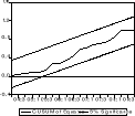
Test de CUSUM de l'estimation 1
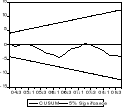
Table des matières
Dédicace i
Remerciements
.......................................................................................................................ii
Sommaire iii
Résumé
.....................................................................................................iv
Abstract
.....................................................................................................v
Liste des abréviations
...............................................................................................................
vi
Liste des tableaux
....................................................................................................................
vii
Annexes
........................................................................ .........................viii
Introduction générale
...................................................................................1
Première partie : la
diversification du portefeuille de crédits : une composante
importante de la rentabilité bancaire
....................................................................................................
10
Introduction première partie
............................................................................
11
Chapitre 1 : les déterminants de
la rentabilité bancaire
.............................................. 12
Section 1 : le portefeuille de crédits
diversifié : un déterminant managérial de la
rentabilité des banques
....................................................................................................
12
I - les éléments d'analyse de la gestion bancaire
.................................................................... 13
I 1 - le bilan bancaire : une présentation explicite du
portefeuille de crédits ......................... 13
I 2 - les opérations hors-bilan
.................................................................................................
15
I 3 - le compte de résultat
.......................................................................................................
15
II - les facteurs explicatifs de la rentabilité des
banques ........................................................ 17
II 1 - la gestion prudentielle et la taille de la banque comme
stimulant de la rentabilité bancaire
...................................................................................................................................
17
II 2 - l'explication de la rentabilité bancaire par les
éléments de la marge d'intermédiation bancaire
...................................................................................................................................
18
Section 2 : les déterminants
macroéconomiques et environnementaux de la rentabilité bancaire
...................................................................................................
20
I - les déterminants macroéconomiques
.................................................................................
21
I 1 - l'impact de la croissance économique
............................................................................
21
I 2 - les effets de l'inflation
....................................................................................................
22
II - les déterminants macro-financiers
....................................................................................
22
II 1 - la taille du secteur bancaire
...........................................................................................
23
II 2 - la concentration bancaire
...............................................................................................
23
Chapitre 2 : analyse théorique de
l'impact de la diversification du portefeuille de crédits sur la
rentabilité bancaire
................................................................................
25
Section 1 : la théorie traditionnelle du
portefeuille .................................................. 25
I - l'essence de la théorie de MARKOWITZ
......................................................................... 26
I 1 - l'idée de départ et les hypothèses
...................................................................................
26
I 2 - les études ultérieures
.......................................................................................................
26
II - l'application de la théorie de Markowitz au
portefeuille de crédits ................................. 28
II 1 - l'approche de la diversification géographique du
portefeuille de crédits ...................... 28
II 2 - la diversification par type de crédit et la
rentabilité bancaire ........................................ 30
Section 2 : la théorie de l'intermédiation
financière ................................................ 31
I - l'étude du marché bancaire
................................................................................................
32
I 1 - la banque comme gestionnaire délégué
du portefeuille de crédit ................................... 33
I 2 - le marché bancaire : marché contestable
et efficient ...................................................... 35
II - la gestion du portefeuille de crédits dans un
marché efficient ......................................... 36
II 1 - la réglementation bancaire en zone BEAC : un
outil en faveur de la division du risque sur le marché bancaire
camerounais
.......................................................................................
37
II 2 - la diversification du portefeuille de crédits pour
une réponse satisfaisante aux besoins de l'économie
...............................................................................................................................
38
Conclusion première partie
............................................................................
40
Deuxième partie : la
diversification du portefeuille de crédits : une composante
insuffisante de la rentabilité bancaire au Cameroun
.................................................................... 41
Introduction deuxième partie
.............................................................................................
42
Chapitre 3 : les effets de la
diversification du portefeuille de crédits sur la rentabilité
bancaire au
Cameroun .........................................................................................................................
43
Section 1 : la démarche
économétrique et l'aspect analytique
.................................... 43
I - Présentation du modèle d'analyse retenu
...........................................................................
44
I 1 - le modèle de régression multiple
....................................................................................
44
I 2 - les outils statistiques d'analyse
.......................................................................................
45
II - cadre d'analyse du modèle
...............................................................................................
46
II 1 - la définition des variables
..............................................................................................
46
II 2 - présentation des données et exposé du
modèle .............................................................
48
Section 2 : Appréciation des facteurs explicatifs de
la rentabilité bancaire au Cameroun ..... 50
I - prolongement de la période et test de normalité
des variables du modèle ........................ 51
I 1 - présentation de l'indice de Hirschman-Herfindal
........................................................... 51
I 2 - trimestrialisation des données annuelles et test de
normalité ......................................... 52
II - stationnarité des variables et estimation du
modèle de la rentabilité bancaire ................. 53
II 1 - les résultats des tests de stationnarité
............................................................................
54
II 2 - l'analyse des résultats et de
l'intérêt de la prise en compte des frais généraux
dans le modèle
.....................................................................................................................................
55
Chapitre 4 : la sensibilité des
résultats bancaires à la taille des banques
............................. 59
Section 1 : l'impact de la taille des banques sur les
vertus de la diversification du portefeuille de crédits au Cameroun
.................................................................................
59
I - présentation des résultats et
appréciation des différents coefficients
................................ 59
I 1 - les résultats de l'estimation de l'équation
de la rentabilité bancaire .............................. 59
I 2 - Appréciation des signes des coefficients
........................................................................ 61
II - la capacité des différentes variables
à expliquer la rentabilité bancaire au Cameroun en absence de la
variable taille des banques
................................................................................
62
II 1 - l'effet des variables managériales
.................................................................................
62
II 2 - l'impact des facteurs macroéconomiques et
macro-financiers sur la rentabilité
bancaire....................................................................................................................................
63
Section 2 : les enseignements du modèle de la
rentabilité bancaire au Cameroun ................. 64
I - les vertus de la bonne tenue des éléments de
la marge d'intermédiation et la rentabilité bancaire au Cameroun
.............................................................................................................
65
I 1 - L'attitude de la rentabilité bancaire face à
la diversification du portefeuille de crédits...65
I 2 - la contribution des charges d'exploitation bancaire
....................................................... 67
II - le rationnement du crédit et l'efficience du
marché bancaire camerounais ..................... 67
II 1 - l'efficience allocationnelle ou fonctionnelle
................................................................. 68
II 2 - diversification du portefeuille de crédits et
réduction du risque.................................... 69
Conclusion deuxième partie
....................................................................................................
70
Conclusion générale
.....................................................................................
71
Bibliographie
................................................................................................
75
| 
