Existence et comportement asymptotique des solutions d'une équation de viscoélasticité non linéaire de type hyperbolique

?????? ?????? ????? ??????? ?????

-

-

????? ???? ?????

?????

BADJI MOKHTAR UNIVERSITY

OF ANNABA UNIVERSITÉ BADJI MOKHTAR

DE ANNABA

Faculté des Sciences
Département de Mathématiques

MÉMOIRE
Présenté en vue de l'obtention du diplôme de

MAGISTER EN MATHÉMATIQUES
ÉCOLE DOCTORALE EN MATHÉMATIQUES

Par
Khaled ZENNIR

Intitulé

Existence et Comportement Asymptotique des

Solutions d~une Equation de Viscoélasticité

Non Linéaire de type Hyperbolique

Dirigé par

Prof. Hocine SISSAOUI

Option

Systemes Dynamiques et Analyse Fonctionnelle

Devant le jury

PRÉSIDENT	B. KHODJA	PROF.	U. B. M. ANNABA
RAPPORTEUR	H. SISSAOUI	PROF.	U. B. M. ANNABA
ÉXAMINATEUR	L. NISSE	M. C.	U. B. M. ANNABA
ÉXAMINATEUR	Y. LASKRI	M. C.	U. B. M. ANNABA
INVITE	B. SAID-HOUARI	Dr.	U. B. M. ANNABA

?????? ?????? ????? ??????? ?????

-

-

????? ???? ?????

?????

BADJI MOKHTAR UNIVERSITY

OF ANNABA UNIVERSITÉ BADJI MOKHTAR

DE ANNABA

Sciences Faculty
Department of Mathematics

THESIS
Submitted for the obtention of

MAGISTER DIPLOMA IN MATHEMATICS
DOCTORAL SCHOOL IN MATHEMATICS

By
Khaled ZENNIR

~~~~

~~~~~~~~~

~~ ~~~~~~~~~~~~

~~~ ~~~~~~~~~~

~~~~~~~~~~~

~~~~ ~~~ of

~~~~~~

~~~~~~~~~

~~~~~ of ~ ~~~~~~~

~~~ ~~~~~~

~~~~~~~~~~~~~~~~

~~~~~~~~~~~~

~~~~~

~~~~~~~~~~

~~ ~~~~ ~~~~~~~~

~~~~~~

Directed by

First Advisor: Prof. Hocine SISSAOUI Second Advisor : Dr. Belkacem SAÏD-HOUARI

Option

Dynamic Systems and Functional Analysis

PRESIDENT	B. KHODJA	PROF.	U. B. M. ANNABA
SUPERVISOR	H. SISSAOUI	PROF.	U. B. M. ANNABA
EXAMINER	L. NISSE	M. C.	U. B. M. ANNABA
EXAMINER	Y. LASKRI	M. C.	U. B. M. ANNABA

Tha1es

lin, the first pace at aLL, vtku eratikkde does to Prof. 1^--/^-. S ISSA-0 k I, VIA.0 stxpervi,sor. t^--te al aus Li,stet/Ls, advi,ces, et/Lcot/traees avid evi,des vie, he as behi,t/Ld this ork. I shall aL aus be 1,vwpressed bu hi,s availabiliku avid the care ith hich he covwes to read avid correct 1/14.b ta1tscript.

mu arm that/Lizs eo to ir.P..,S.411-1^-1^-0W1-121, ho supervi,sed this thesis

1,th great pati,et/Lce avid Izi,t/Ldt/Less. f-te as aloft to vtkoti,vate each step of 1/14.b

orn lob reLevat/Lt revt/tarizs avid Let vte abbe to 00N/o/Lae 1,1/L vt/tu research, beei,t/LI/Li,vLe bu the D.ES Stv.0(U I txt/Li,versiku of sizi,lzda. I that/Liz hi,vt/t, verb si,t/LcereLb for hi,s availabiliku eve at a di,stat/Lce, ith hi,vt/t. I have a Lot of ft/tvL to orn.

I ish to that/Liz Prof P.. ICI-I^-Opy.4, ho vtkalzes vte the hot/tour of chai,ri,vLe the jt/tru of vtku defet/Lse.

~ avw verb crateful, to z)r. L. MSS& avi,of 1)r. y LASICRI to have agreed to resci,t/Ld this thesis avid to be part of vtku defet/Lse pateL.

of course, this thesis 1,s the cyLvtki,vLati,ovL of vtkat/Lb bears of sttxdu. 1 avA. 1,o,debted to aLL those ho e[doed vt/te ot/L the road of vtkathevtkati,cs.

~ that/Liz from. vtku heart, vtku teachers hose et/Lcokraeed vtke dt/tri,vLe 1/14.b studies avid have di,stracted vt/te the vtkathevtkati,cs.

I thi,vLlz for vtku paret/Lts, hose the orn could t/Lot succeed ithout their et/LdLess support avid et/LcokraeevtkevLt. Theo ^-Rost i,t/L the reaLizati,ovL of this

ork, the cyLvtki,vLati,ovL of theix efforts at/Ld express vtku vtkost affecti,ovote eratikkde.

Contents

1	Preliminary		1
	1.1	Banach Spaces - Definition and Properties	2
		1.1.1 The weak and weak star topologies	3
		1.1.2 Hilbert spaces	4
	1.2	Functional Spaces	6
		1.2.1 The L^p (l) spaces	6
		1.2.2 The Sobolev space W^m'^p(1)	8
		1.2.3 The L^p (0, T, X) spaces	10
		1.2.4 Some Algebraic inequalities	12
	1.3	Existence Methods	14
		1.3.1 The Contraction Mapping Theorem	14
		1.3.2 Gronwell's lemma	14
		1.3.3 The mean value theorem	15
2	Local Existence		17
	2.1 Local Existence Result		18
3	Global Existence and Energy Decay		39
	3.1	Global Existence Result	40
	3.2	Decay of Solutions	46
4	Exponential Growth		59
	4.1 Growth result		60

Abstract

Our work, in this thesis, lies in the study, under some conditions on p, m and the functional g, the existence and asymptotic behavior of solutions of a nonlinear viscoelastic hyperbolic problem of the form

utt ~ Xu ~ W~ut + _Rt g(t - s)iu(s, x)ds

0

+a jutj^m~2 ut = b juj^p~2 u, x 2 l, t > 0

u(0,x) = u0 (x), x 2 ~ ut (0,x) = u1 (x), x 2 ~

u(t,x) = 0, x 2 [', t > 0

₈

<>>>>>>>>>>>>>>> >

>>>>>>>>>>>>>>>>:

, (P)

where is a bounded domain in R^N (N ~ 1), with smooth boundary [', a, b, w are positive constants, m ~ 2, p ~ 2, and the function g satisfying some appropriate conditions.

Our results contain and generalize some existing results in literature. To prove our results many theorems were introduced.

Keywords: Nonlinear damping, strong damping, viscoelasticity, nonlinear source, local solutions, global solutions, exponential decay, polynomial decay, growth.

Résumé

Notre travail, dans ce memoire consiste a étudier l'éxistence et le comportement asymptotique des solutions d'un problème de viscoelasticité non lineaire de type hyperbolique suivant:

utt ~ Xu ~ W~ut + _Rt g(t - s)iu(s, x)ds

0

+a jutj^m~2 ut = b juj^p~2 u, x 2 l, t > 0

u(0,x) = u0 (x), x 2 ~ ut (0,x) = u1 (x), x 2 ~

u(t,x) = 0, x 2 [', t > 0

₈

<>>>>>>>>>>>>>>> >

>>>>>>>>>>>>>>>>:

, (P)

on, est un domaine borné de R^N (N ~ 1), avec frontière assez regulière [1, a, b, w sont des constantes positives, n-i ~ 2, p ~ 2, et la fonction g satisfaite quelques conditions.

Nos résultats contiennent et généralisent certains résultats d'existences dans la littérature. Pour la preuve, beaucoup théorèmes ont été présentés

Mots dlés: Dissipation nonlinéaire, viscoelasticité, source nonlinéaire, solutions locale, solutions globale, décroissance exponentielle de l'énergie, décroissance polynomiale, croissement.

iv

Notations

a : bounded domain in R^N.

~ : topological boundary of a.

x = (xi, x2, ...,xN) : generic point of R^N.

dx = dx1dx2...dxN : Lebesgue measuring on a.

Vu : gradient of u.

Au : Laplacien of u.

f+, f^- : max(f, 0), max(--f,0).

a.e : almost everywhere.

+

1 p^,

= 1.

p^' : conjugate of p, i.e 1

p

D(a) : space of differentiable functions with compact support in a.

D^'(a) : distribution space.

C^k (a) : space of functions k--times continuously differentiable in a. Co (a) : space of continuous functions null board in a.

Lp (a) : Space of functions p--th power integrated on a with measure of dx.

1
p

.

11f11_p = (1₁ I f(x)Ip)

W^1,p (a) = {u E L^p (a) , Vu E (L^p (a))^N1 .

1

^p .

= (11ur_p+ 11Vur_p)

W 1;p

0(a) : the closure of D (a) in W^1,p (a). W ^~1;^p0(a) : the dual space of W0 "^p (a).

H : Hilbert space. H1 0 =W0 ^1;2 .

If X is a Banach space

T

Lp (0, T; X) = {f : (0, T) --> X is measurable ; f 11f(t)111 dt < oo} .

0

{ )

L^°° (0, T; X) = f : (0, T) --> X is measurable ;ess -- sup 11f(t)11^p_X < oo .

tE(0,T)

C^k ([0, T] ; X) : Space of functions k--times continuously differentiable for [0, T] --> X.

D ([0, T] ; X) : space of functions continuously differentiable with compact support in [0, T] . Bx = Ix E X; 11x11 < 1} : unit ball.

Introduction

In this thesis we consider the following nonlinear viscoelastic hyperbolic problem

utt - Au - wAut +

g(t - s)Au(s,x)ds

t

f

0

₈

<>>>>>>>>>>>>> >

>>>>>>>>>>>>>>:

, (1)

+a1ut1^m-2 ut = b 1u1^1-2 u, x E , t > 0

u (0, x) = up (x) , ut (0, x) = ui (x) , x E Q u (t, x) = 0, x E 1^-1, t > 0

where Q is a bounded domain in R^N (N > 1), with smooth boundary F, a, b, w are positive constants, and n7, > 2, p > 2. The function g(t) is assumed to be a positive nonincreasing function defined on R^#177; and satisfies the following conditions:

(G1). g : R^#177; -! R^#177; is a bounded C¹-function such that

g(0) > 0, 1 - I g(s)ds = l > 0.

0

(G2). g(t) > 0, g^'(t) < 0, g(t) < -~g^'(t), V t > 0, > 0.

In the physical point of view, this type of problems arise usually in viscoelasticity. This type of problems have been considered first by Dafermos [12], in 1970, where the general decay was discussed. A related problems to (1) have attracted a great deal of attention in the last two decades, and many results have been appeared on the existence and long time behavior of solutions. See in this directions [2, 3, 5 - 8, 18, 29, 33, 34, 38] and references therein.

In the absence of the strong damping Aut, that is for w = 0, and when the function g vanishes identically ( i.e. g = 0), then problem (1) reduced to the following initial boundary damped wave equation with nonlinear damping and nonlinear sources terms.

utt - Au + a1ut1^m-2 ut = b 1u1^1-2 u. (2)

Some special cases of equation (2) arise in quantum field theory which describe the motion of charged mesons in an electromagnetic field.

Equation (2) together with initial and boundary conditions of Dirichlet type, has been extensively
studied and results concerning existence, blow up and asymptotic behavior of smooth, as well

vi

as weak solutions have been established by several authors over the past three decades. Some interesting results have been summarized by Said-Houari in his master thesis [42].

For b = 0, that is in the absence of the source term, it is well known that the damping term a utj^m-2 ut assures global existence and decay of the solution energy for arbitrary initial data ( see for instance [17] and [21]).

For a = 0, the source term causes finite-time blow-up of solutions with a large initial data ( negative initial energy). That is to say, the norm of our solution u(t, x) in the energy space reaches +oc when the time t approaches certain value T^* called " the blow up time", ( see [1] and [20] for more details).

The interaction between the damping term a utj^m-2 ut and the source term b uj^p-2 u makes the problem more interesting. This situation was first considered by Levine [23,24] in the linear damping case (m = 2), where he showed that solutions with negative initial energy blow up in finite time T^*. The main ingredient used in [23] and [24] is the " concavity method" where the basic idea of this method is to construct a positive function L(t) of the solution and show that for some 'y > 0, the function L^-Y(t) is a positive concave function of t. In order to find such 'y, it suffices to verify that:

d^2L^-Y(t)	= --yL^-"^-2(t) [LL^'' - (1 + y)L^'2(t)] 0, Vt ~ 0.
dt^2

This is equivalent to prove that L(t) satisfies the differential inequality

LL^''--(1+'y)L^'2(t) ~ 0, Vt ~ 0.

Unfortunately, this method fails in the case of nonlinear damping term (m > 2).

Georgiev and Todorova in their famous paper [14], extended Levine's result to the nonlinear damping case (m > 2). More precisely, in [14] and by combining the Galerkin approximation with the contraction mapping theorem, the authors showed that problem (2) in a bounded domain with initial and boundary conditions of Dirichlet type has a unique solution in the interval [0, T) provided that T is small enough. Also, they proved that the obtained solutions continue to exist globally in time if m ~ p and the initial data are small enough. Whereas for p > m the unique solution of problem (2) blows up in finite time provided that the initial data are large enough. ( i.e. the initial energy is sufficiently negative).

This later result has been pushed by Messaoudi in [35] to the situation where the initial energy E(0) < 0. For more general result in this direction, we refer the interested reader to the works of Vitillaro [47], Levine [25] and Serrin and Messaoudi and Said-Houari [32].

In the presence of the viscoelastic term (g =6 0) and for w = 0, our problem (1) becomes

₈

<>>>>>>>>>>>>> >

>>>>>>>>>>>>>>:

t

f

0

utt -- Au +

g(t -- s)Au(s,x)ds

+alutl^m-2 ut = b lul^1-2 u, x E Q, t > 0 (³)

u (0, x) = up (x) , ut (0, x) = ui (x) , x E Q

u (t, x) = 0, x E 1^-1, t > 0

For a = 0, problem (3) has been investigated by Berrimi and Messaoudi [3]. They established the local existence result by using the Galerkin method together with the contraction mapping theorem. Also, they showed that for a suitable initial data, then the local solution is global in time and in addition, they showed that the dissipation given by the viscoelastic integral term is strong enough to stabilize the oscillations of the solution with the same rate of decaying ( exponential or polynomial) of the kernel g. Also their result has been obtained under weaker conditions than those used by Cavalcanti et al [7], in which a similar problem has been addressed.

Messaoudi in [29], showed that under appropriate conditions between m, p and g a blow up and global existence result, of course his work generalizes the results by Georgiev and Todorova [14] and Messaoudi [29].

One of the main direction of the research in this field seems to find the minimal dissipation such that the solutions of problems similar to (3) decay uniformly to zero, as time goes to infinity. Consequently, several authors introduced different types of dissipative mechanisms to stabilize these problems. For example, a localized frictional linear damping of the form a(x)ut acting in sub-domain w c Q has been considered by Cavalcanti et al [7]. More precisely the authors in [6] looked into the following problem

utt -- Au +

t I 0

g(t -- s)Au(s,x)ds + a(x)ut + lul^~ u = 0. (4)

for 7 > 0, g a positive function and a : Q -> IR⁺ a function, which may be null on a part of the domain Q.

By assuming a(x) > a0 > 0 on the sub-domain w c Q, the authors showed a decay result of an exponential rate, provided that the kernel g satisfies

-- (1g(t) < g⁰(t) < --(2g(t), t > 0, (5)

and _MgML1(0,1) is small enough.

This later result has been improved by Berrimi and Messaoudi [2], in which they showed that the viscoelastic dissipation alone is strong enough to stabilize the problem even with an exponential rate.

In many existing works on this field, the following conditions on the kernel

g^'(t) -~g'(t), t ~ 0, p ~ 1, (6)

is crucial in the proof of the stability.

For a viscoelastic systems with oscillating kernels, we mention the work by Rivera et al [36]. In that work the authors proved that if the kernel satisfies g(0) > 0 and decays exponentially to zero, that is for p = 1 in (6), then the solution also decays exponentially to zero. On the other hand, if the kernel decays polynomially, i.e. (p > 1) in the inequality (6), then the solution also decays polynomially with the same rate of decay.

In the presence of the strong damping (w > 0) and in the absence of the viscoelastic term (g = 0), the problem (1) takes the following form

8 <>>>>>>> >>>>>>>:

utt ~ u ~ !~ut + a jutj^m-2 ut = b juj^p-2 u, x 2 ~, t > 0 u(0,x) = u0 (x), u2 (0,x) = u1 (x), x 2 ~ (7) u(t,x) = 0, x 2 [', t > 0

Problem (7) represents the wave equation with a strong damping ~ut. When m = 2, this problem has been studied by Gazzola and Squassina [13]. In their work, the authors proved some results on well posedness and asymptotic behavior of solutions. They showed the global existence and polynomial decay property of solutions provided that the initial data is in the potential well.

The proof in [13] is based on a method used in [19]. Unfortunately their decay rate is not optimal, and their result has been improved by Gerbi and Said-Houari [16], by using an appropriate modification of the energy method and some differential and integral inequalities.

Introducing a strong damping term Iu makes the problem from that considered in [42] and [14], for this reason less results where known for the wave equation with strong damping and many problem remain unsolved. ( See [13] and the recent work by Gerbi and Said-Houari [15]).

In this thesis, we investigated problem (1), in which all the damping mechanism have been considered
in the same time ( i.e. w > 0, g =6 0, and m ~ 2), these assumptions make our problem different

form those studied in the literature, specially the blow up result / exponential growth of solutions (chapter4).

This thesis is organized as follows:

Chapter1:

In this chapter we introduce some notation and prepare some material needed for our work. The main results of this chapter such as: the L^p-- spaces, the Sobolev spaces, differential and integral inequalities and other theorems of functional analysis, can found in the books [4] and [43]. Chapter2:

This chapter is devoted to the study of the local existence result, the main ingredient used in this chapter is the Galerkin approximations ( the compactness method) introduced in the book of Lions [26], together with the fix point method.

Indeed, we consider first for u 2 C ([0, T] , H¹ 0) given, the following problem

vtt - Lv - WLvt + _Zt g(t - s)Lv(s, x)ds + ajvtj^m~2 vt = bjuj^p~2 u, x 2 , t > 0 (8)

0

with the initial data

v (0,x) = u0 (x), vt (0,x) = u1 (x),x 2 (9)

and boundary conditions of the form

v (t, x) = 0, x 2 [', t > 0, (10)

and we will show that problem (8) - (10) has a unique local solutions v by the Faedo-Galerkin method, which consists in constructing approximations of the solution, then we obtain a priori estimates necessary to guarantee the convergence of these approximations. We recall here that the presence of nonlinearity on the damping term a vtj^m~2 vt forces us to go until the second a priori estimate. We point out that the contraction semigroup method fails here, because of the presence of the nonlinear terms.

Once the local solution v exists, we will use the contraction mapping theorem to show the local existence of our problem (1). This will be done under the assumption that T is required to be small enough (see formula (2.77)).

Chapter 3:

Our main purpose in this chapter is tow-fold:

First, we introduce a set W defined in (3.5) called " the potential well" or " stable set" and we show that if we restrict our initial data in this set, then our solution obtained in chapter 2 is global in time, that is to say, the norm

kutM2 + VuM₂ ,

in the energy space L²(l) x H¹ ₀(l) of our solution is bounded by a constant independent of the time t.

Second, We show that, if our solution is global in time, ( i.e. by assuming that the initial data u0 2 W) and if our function g satisfies the condition (6) ( for p = 1), then our solution decays time asymptotically to zero. More precisely we prove that the decay rate is of the form (1 + t)21(2_m) if n-i > 2, whereas for n-i = 2, we obtain an exponential decay rate. (See Theorem 3.2.1). The main tool used in our proof is an inequality due to Nakao [37], in which this inequality has been introduced in order to study the stability of the wave equation, but it is still works in our problem. Chapter 4:

In this chapter we will prove that if the initial energy E(0) of our solution is negative ( this means that our initial data are large enough), then our local solutions in bounded and

kutM2 + VuM₂ - 1

as t tends to +oo. In fact it will be proved that the L^p--norm of the solution grows as an exponential function. An essential tool of the proof is an idea used by Gerbi and Said-Houari [15], which based on an auxiliary function ( which is a small perturbation of the total energy), in order to obtain a differential inequality leads to the exponential growth result provided that the following conditions

_Z

0

p - 2

g(s)ds < p _ 1,

holds.

Chapter 1

Preliminary

Abstract

In this chapter we shall introduce and state some necessary materials needed in the proof of our results, and shortly the basic results which concerning the Banach spaces, the weak and weak star topologies, the I^I space, Sobolev spaces and other theorems. The knowledge of all this notations and results are important for our study.

1.1 Banach Spaces - Definition and Properties

We first review some basic facts from calculus in the most important class of linear spaces "Banach spaces".

Definition 1.1.1 A Banach space is a complete normed linear space X. Its dual space X^' is the linear space of all continuous linear functional f : X --> R.

Proposition 1.1.1 ([43])

X^' equipped with the norm 11.11_x, defined by

II/11x^, = sup flf(u)I : Ilull 1}, (1.1)

is also a Banach space.

We shall denote the value of f 2 X^' at u 2 X by either f(u) or (f, u)x^,,x
·

Remark 1.1.1 ([43]) From X^' we construct the bidual or second dual X^'' = (X^')^'. Furthermore, with each u 2 X we can define cp(u) 2 X^'' by cp(u)(f) = f(u), f 2 X^', this satisfies clearly Ip(x)1 < Mull . Moreover, for each u 2 X there is an f 2 X^' with f(u) = Mull and 11f11 = 1, so it follows that Ip(x)1 = Mull .

Definition 1.1.2 Since cp is linear we see that

cp : X --> X^'',

is a linear isometry of X onto a closed subspace of X^'', we denote this by

X c-- X^''.

Definition 1.1.3 If cp ( in the above definition) is onto X^'' we say X is reflexive, X c-^--^,' X^''.

Theorem 1.1.1 ([4], Theorem III.16)

Let X be Banach space. Then, X is reflexive, if and only if,

Bx = Ix 2 X :114 <11,
is compact with the weak topology a (X, X^') . (See the next subsection for the definition of a (X, X^'))

Definition 1.1.4 Let X be a Banach space, and let (u_n)_nEN be a sequence in X. Then u_n converges strongly to u in X if and only if

lim

n-->o

Ilun -- ullx = 0,

and this is denoted by un --p u, or lim n-->o

Un = U.

1.1.1 The weak and weak star topologies

Let X be a Banach space and f E X^'. Denote by

cpf : X --> R

x i--> Wf(x),

(1.2)

when f cover X^', we obtain a family (cpf)_fcx, of applications to X in R.

Definition 1.1.5 The weak topology on X, denoted by a (X, X^') , is the weakest topology on X for which every (pf)_fcx, is continuous.

We will define the third topology on X^', the weak star topology, denoted by a (X^', X) . For all

x E X. Denote by

cp_x : X^' --> R

f i^- wx(f) = (f, x)x,,x, (1.3)

when x cover X, we obtain a family (cp_x)_xcx, of applications to X^' in R.

Definition 1.1.6 The weak star topology on X^' is the weakest topology on X^' for which every (4x)xcx^, is continuous.

Remark 1.1.2 ([4]) Since X C X^'', it is clear that, the weak star topology a (X^', X) is weakest then the topology a (X^', X^''), and this later is weakest then the strong topology.

Definition 1.1.7 A sequence (u_n) in X is weakly convergent to x if and only if

1im n-->o

f(un) = f(u),

for every f E X^', and this is denoted by u_n --, u.

Remark 1.1.3 ([42], Remark 1.1.1)

1. If the weak limit exist, it is unique.

2. If u_n --> u E X (strongly), then u_n --, u (weakly).

3. If dim X < +oo, then the weak convergent implies the strong convergent.

Proposition 1.1.2 ([43])

On the compactness in the three topologies in the Banach space X :

1- First, the unit ball

B Ix E X : 11x11 < 1}, (1.4)

in X is compact if and only if dim(X) < oc.

2- Second, the unit ball B^' in X^' (The closed subspace of a product of compact spaces) is weakly compact in X^' if and only if X is reflexive.

3- Third, B^' is always weakly star compact in the weak star topology of X^'.

Proposition 1.1.3 ([4], proposition III.12)

Let (f_n) be a sequence in X^'. We have:

[ ]

~

1. f_m * f in a (X^', X) [f_n(x) ! f(x), Vx 2 X].

2. If fTh - f (strongly), then _fTh - f, in a (X^', X^''), If f_m - f in a (X^',X^''), then f_m - f, in a (X^',X).

~

3. If _fTh - f, in a (X^',X), then kf_nk is bounded and kfk ~ liminf Mf_nM.

~

4. If _fTh - f, in a (X^', X) and x, -p x (strongly) in X, then f_n(x_n) -p f(x).

~

1.1.2 Hilbert spaces

The proper setting for the rigorous theory of partial differential equation turns out to be the most important function space in modern physics and modern analysis, known as Hilbert spaces. Then, we must give some important results on these spaces here.

Definition 1.1.8 A Hilbert space H is a vectorial space supplied with inner product (u,v) such that Jkuk = (u, u) is the norm which let H complete.

Theorem 1.1.2 ([42], Theorem 1.1.1)

Let _(un)mEN is a bounded sequence in the Hilbert space H, then it possess a subsequence which converges in the weak topology of H.

Theorem 1.1.3 ([42], Theorem 1.1.2)

In the Hilbert space, all sequence which converges in the weak topology is bounded.

Theorem 1.1.4 ([42], Corollary 1.1.1)

Let _(un)mEN be a sequence which converges to u, in the weak topology and _(vfl)mEN is an other sequence which converge weakly to v, then

lim Th-400

(vn,un) = (v,u). (1.5)

Theorem 1.1.5 ([42], Theorem 1.1.3)

Let X be a normed space, then the unit ball

{ }

B' = i 2 X^' : klk < 1 , (1.6)

of X^' is compact in a (X^', X).

Proposition 1.1.4 ([42], Proposition 1.1.1)

Let X and Y be two Hilbert spaces, let (un)nEN _E X be a sequence which converges weakly to u E X, let A E £(X, Y ). Then, the sequence (A (u_n))_nEN converges to A(u) in the weak topology of Y.

Proof. For all u E X, the function

u i-- (A(u), v)

is linear and continuous, because

1(A(u), v)1 < IIAII,c(x, _IT) IIuII_X IIvII_I , Vu E X, v E Y. So, according to Riesz theorem, there exists w E X such that

(A(u), v) = (u, w), Vu E X.

Then,

lim n-->o

(A (un) , v) = lim n-->o

(um, w)

= (u, w) = (A(u), v). (1.7)

This completes the proof.

1.2 Functional Spaces

1.2.1 The LP (Q) spaces

Definition 1.2.1 Let 1 < p < oo, and let Q be an open domain in Rⁿ, n 2 N. Define the standard Lebesgue space L^P(Q), by

L^P(Q) =

8 < :

f : Q -- >R : f is measurable and I n

If(x)1^P dx < 1

9 = ;

· (1.8)

Notation 1.2.1 For p 2 R and 1 < p < oo, denote by

1 P

·

(1.9)

0 Z

kfk_p = @ 1f(x)r dx
n

If p = oo, we have

L°°(Q) = If : Q -- R : f is measurable and there exists a constant C

(1.10)

such that, 1f(x)1 < C a.e in Q1.

Also, we denote by

11/11₀₀ = Inf {C, If(x)1 < C a.e in Q} . (1.11)

+

1
q

=1.

1

Notation 1.2.2 Let 1 ~ p ~ 1_; we denote by q the conjugate of p i.e.

P

Theorem 1.2.1 ([48])

It is well known that L^P(Q) supplied with the norm 11.11_p is a Banach space, for all 1 < p < 00. Remark 1.2.1 In particularly, when p = 2, L² (Q) equipped with the inner product

(f, 94²(n) = f

n f(x)g(x)dx, (1.12)

is a Hilbert space.

Theorem 1.2.2 ([43], Corollary 3.2)

For 1 < p < oo, L^P(Q) is reflexive space.

Some integral inequalities

We will give here some important integral inequalities. These inequalities play an important role in applied mathematics and also, it is very useful in our next chapters.

Theorem 1.2.3 ([48], Holder's inequality )

Let 1 < p < oo. Assume that f 2 L^P(Q) and g 2 L^q(Q), then, fg 2 L¹(Q) and

fgl dx < 11/4 mgmq (1.13)

Corollary 1.2.1 (Holder's inequality - general form)

Lemma 1.2.1 Let f1, 12, ...fk be k functions such that, fi 2 L^A(Q), 1 < i < k, and

1

1
p

=

+

P1

1

+ ::: +

P2

1 < 1.

Pk

Then, the product f1f2
·
·
·fk 2 L^P(1) and If1f2
·
·:fkl_p ~ kf1k_p1
·
·
·11fklIp_k
·

Lemma 1.2.2 ( [48], Young's inequality)

r

=

1
p

+

1
q

-- 1 > O. Then

Let f 2 L^P(I18) and g 2 L^q(118) with 1 < p < oo, 1 < q < 1 and 1 f * g 2 UM and

MI * ql1L^7-(R) < MIlli,p(R)11q1lifl(R)- (1.14)

Lemma 1.2.3 ([43], Minkowski inequality) For 1 < p < oo, we have

Mu +OLP < 11⁷/11/,/^, +11v1ILP (1.15)

Lemma 1.2.4 ([43])

1

Let 1 < p < r < q,

r

1--a

+

q

, and 1 < a < 1. Then

a
p

=

kukLr ~11u117,p kuk1~~

Lq (1.16)

Lemma 1.2.5 ([43])

If _au (Q) < oo, 1 < p < q < oo, then L^q y L^P, and

1
p

uhp < it(Q)

1

q kukLq :

1.2.2 The Sobolev space Wm,p(I)

Proposition 1.2.1 ([26])

Let a be an open domain in le, Then the distribution T 2 D^'(a) is in L^P(a) if there exists a function f 2 L^P(a) such that

(T, (P) = I

f(x)cp(x)dx, for all cp 2 D(a),

where 1 < p < oo, and it's well-known that f is unique.

Definition 1.2.2 Let m 2 N and p 2 [0, oo] . The W^m,P(a) is the space of all f 2 L^P(a), defined

as

W^m'^P(a) = 2 L^P(a), such that O^af 2 L^P(a) for all a 2 N^tm such that

jj (1.17)

= j=1ai < m, where, a^s = @~2

2 ::@~n

n g:

Theorem 1.2.4 ([9])

W^m,P(a) is a Banach space with their usual norm

mi,vm^,pm= E jj~m

11a^sf11Lp , 1 < p < oo, for all f 2 W^rd'(a). (1.18)

Definition 1.2.3 Denote by Wr'^P(a) the closure of D(a) in W^m,P(a).

Definition 1.2.4 When p = 2, we prefer to denote by W^{m 2}(a) = H^t (a) and Wc7² (a) = H^m0 (a) supplied with the norm

0 11/11H-(n) = (11.9711L2)2) jj~m

1 2

;

(1.19)

which do at H^tm (a) a real Hilbert space with their usual scalar product

(u, v) (n) = E J O^auo^avdx (1.20)

101<m n

Theorem 1.2.5 ([42], Proposition 1.2.1)

1) H^t (a) supplied with inner product (.,.)H.(n) is a Hilbert space.

2) If m > m^', H^tm (a) y H^m' (a), with continuous imbedding .

Lemma 1.2.6 ([26])

Since D(a) is dense in H^m₀ (a), we identify a dual H' (a) of H^m₀ (a) in a weak subspace on a, and we have

D(a) y H^m0 (a) y L² (a) y H^' (a) y D⁰(a),

Lemma 1.2.7 (Sobolev-Poincaré's inequality) If

m - 2,

2 ~ q ~

2m m > 3

q ~ 2, m = 1,2,

then

kuk_q ~ C(q, ) VuM₂ , (1.21)

for all u 2 H1 0 (1).

The next results are fundamental in the study of partial differential equations

Theorem 1.2.6 ([9] Theorem 1.3.1)

Assume that is an open domain in R^N (N ~ 1), with smooth boundary F. Then,

(i) if 1 p m, we have W¹' c L^q(l), for every q 2 [p, p^*] , where p^* = mp .

m ~ p

(ii) if p = m we have W^1' C L^q(1), for every q 2 [p, oc). (iii) if p > m we have W^1' C L^°°(l) fl C^0'(l), where a = - m p

.

Theorem 1.2.7 ([9] Theorem 1.3.2)

If 1 is a bounded, the embedding (ii) and (iii) of theorem 1.1.4 are compacts. The embedding (i) is compact for all q 2 [p, p^*).

Remark 1.2.2 ([26])

For all çü 2 H²(1), LIço 2 L²(1) and for F sufficiently smooth, we have

ko(t)MH2(~) C _{k~co(t)ML2(~)} . (1.22)

Proposition 1.2.2 ([43], Green's formula) For all u 2 H²(~), v 2 H¹(1) we have

f-

ZLuvdx = ~

fVuVvdx - @~

@u vda, (1.23) @~

@u

where is a normal derivation of u at F.

@~

1.2.3 The LP (0, T, X) spaces

Definition 1.2.5 Let X be a Banach space, denote by L^p(0, T, X) the space of measurable functions

f : ]0,T[ -- X t' f(t)

such that

(

T I 0

11 f (t)111 dt)

= 11I11LP(0,T,x) < oc, for 1 < p < oo. (1.24)

If p = oo,

11I11L.0(0,T,x) = sup tE]0,T[

ess 11f(t)11x - (1.25)

Theorem 1.2.8 ([42])

The space L^p(0, T, X) is complete.

We denote by D' (0, T, X) the space of distributions in ]0, T[ which take its values in X, and let us define

D' (0,T, X) = r (D ]0,T[, X) ,

where r (0, (p) is the space of the linear continuous applications of _q to (p. Since u 2 D' (0, T, X) , we define the distribution derivation as

au

at ((p) = u (4)

t ' Vcp 2 D (]0,T[) , (1.26)

d

and since u 2 L^p (0, T, X) , we have

u((p) =

T I 0

u(t)(p(t)dt, Vcp 2 D (]0,T[) . (1.27)

We will introduce some basic results on the L^p(0, T, X) space. These results, will be very useful in the other chapters of this thesis.

Lemma 1.2.8 ([26] Lemma 1.2 )

0 f

Let f 2 L^p(0, T, X) and _@t2 L^p(0, T, X), (1 < p < oo) , then, the function f is continuous from [0, 7¹] to X.i.e. f 2 C¹(0, T, X).

Lemma 1.2.9 ([26])

Let çü = ]0, T[x an open bounded domain in RxRⁿ, and let _g,1, g are two functions in L (]0, T[, L^q(c)), 1 < q < 1 such that

Mg,LMLq(0,T,Lq(~)) ~ C, V,LL 2 N (1.28)

and

g,1 --p g in çü,

then

g,1 - g in L (ço).

Theorem 1.2.9 ([9], Proposition 1.4.17) L^1(0, T, X) equipped with the norm k.kLp(0,T,x), 1 < p < 1 is a Banach space. Proposition 1.2.3 ([14]) 1 Let X be a reflexive Banach space, X^' it's dual, and 1 p < oc, 1 q < oc, p dual of L^P(0, T, X) is identify algebraically and topologically with L^q(0, T, X^').

+

1 q

= 1. Then the

Proposition 1.2.4 ([9])

Let X, Y be to Banach space, X c Y with continuous embedding, then we have L^P(0, T, X) c L^P(0, T, Y ) with continuous embedding.

The following compactness criterion will be useful for nonlinear evolution problems, especially in the limit of the non linear terms.

Proposition 1.2.5 ([26]).

Let B0, B, B1 be Banach spaces with B0 C B C B1, assume that the embedding B0 ,! B is compact and B ,! B1 are continuous. Let 1 < p < oc, 1 < q < oc, assume further that B0 and B1 are reflexive.

Define

W ~ {u 2 L^° (0, T, B0) : u^' 2 L^q (0, T, B1)}. (1.29)

Then, the embedding W ,! L^p (0, T, B) is compact.

1.2.4 Some Algebraic inequalities

Since our study based on some known algebraic inequalities, we want to recall few of them here. Lemma 1.2.10 ([48],The Cauchy-Schwarz inequality)

Every inner product satisfies the Cauchy-Schwarz inequality

(x₁, X2) kxiM X2M (1.30)

The equality sign holds if and only if X1 and X2 are dependent.

Young's inequalities :

Lemma 1.2.11 For all a, b 2 R⁺, we have

ab < 8a² + b2

48, (1.31)

where 8 is any positive constant.

Proof. Taking the well-known result

(28a -- b)² ~ 0 Va, b 2 R

for all 8 > 0, we have

48²a² + b² - 48ab ~ 0.

This implies

48ab < 48²a² + b2

consequently,

ab < 8a² + 48 1 b2.

This completes the proof.

Lemma 1.2.12 ([43])

For all a, b ~ 0, the following inequality holds

_bq

+ ;

q

_a°

ab < p

1
q

= 1.

+

1

where, p

Proof. Let G = (0,1), and f : G --> IR is integrable, such that

p log a, 0 < x < 1

q log b, 1

P

P

< x < 1

)

₈

<>

>:

f(x) =

1
q

= 1.

+

for all a, b > 0 and 1

P

Since cp(t) = e^t is convex, and using Jensen's inequality

(,⁰(¹

(1.32)

,u (G) If (x)dx) <

-- ,u (G)

f cp (f (x)) dx.

G G

Consequently, we have

_Z

1

~ (G)

G

1

I

0 _of (x) dx =

1 /p 1

I

0 _ep log adx + I

1/p

cp (f(x)) dx =

_eq log b_dx

1 / p

I

0

1

I

1/p

=

ap dx +

bq dx

(a^p) + (1 -- ) b^q .

=

P

(1.33)

ap	bq
=		+ P	, q

G

where, ,u (G) = 1 and

40 ( ¹ I

f (x)dx = e(f0 f (x)dx) = e (V/p p log _{adx#177;fi1/p} q log bdx)

= _e(log a#177;log b) = _clog ab

= ab. (1.34)

Using (1.32), (1.33) and (1.34) to conclude the result.

1.3 Existence Methods

1.3.1 The Contraction Mapping Theorem

Here we prove a very useful fixed point theorem called the contraction mapping theorem. We will apply this theorem to prove the existence and uniqueness of solutions of our nonlinear problem.

Definition 1.3.1 Let f : X - X be a map of a metric space to itself. A point x 2 X is called a fixed point off if f(x) = x.

Definition 1.3.2 Let (X, dx) and (Y, dY ) be metric spaces. A map çü : X -p Y is called a contraction if there exists a positive number C < 1 such that

dy (ço(x),ço(y)) Cdx(x,y), (1.35)

for all x,y 2 X.

Theorem 1.3.1 (Contraction mapping theorem [45] )

Let (X, d) be a complete metric space. If çü : X -p X is a contraction, then çü has a unique fixed point.

1.3.2 Gronwell's lemma

Theorem 1.3.2 ( In integral form)

Let T > 0, and let çü be a function such that, çü 2 L¹(0, T), çü ~ 0, almost everywhere and q be a function such that, q 2 L¹(0,T), q ~ 0, almost everywhere and qço 2 L¹ [0, T], Ci, C2 ~ 0. Suppose that

q(t) ~ Ci + C2 _Zt ço(s)q(s)ds, for a.e t 2 ]0,T[, (1.36)

0

then,

t

_{0 1}

_f

0

q(t) Ci exp _@C2 '(s)ds ^A , for a.e t 2 ]0,T[. (1.37)

Proof. Let

F(t) = C1 + C2 _Zt ço(s)q(s)ds, for t 2 [0, T], (1.38)

0

we have,

q(t) F(t),

From (1.38) we have

F^'(t) = C2ço(t)q(t)

~ C2ço(t)A(t), for a.e t 2 ]0,T[. (1.39)

d

₈

<

:

dt

Consequently,

_{0 1 9}

f t =

F (t) exp @_ C2'(s)ds _A 0, (1.40)

0

;

then,

t

_{0 1}

_f

F (t) ~ Ci exp _@C2 (s)ds _A , for a.e t 2 ]0, T[. (1.41)

0

Since q F, then our result holds.

In particle, if C1 = 0, we have q = 0 for almost everywhere t 2 ]0, T[.

1.3.3 The mean value theorem

Theorem 1.3.3 Let G : [a, b] -p be a continues function and çü : [a, b] -p is an integral positive function, then there exists a number x in (a, b) such that

_Zb G(t)cp(t)dt = G(x) _Zb ço(t)dt. (1.42)

a a

m _Zb ço(t)dt ~ _Zb G(t)ço(t)dt M _Zb ço(t)dt. (1.46)

a a a

In particular for ço(t) = 1, there exists x 2 (a, b) such that

_Zb G(t)dt = G(x) (b - a). (1.43)

a

Proof. Let

m = inf {G(x), x 2 [a, b]} (1.44)

and

M = sup {G(x), x 2 [a, b]} (1.45)

of course m and M exist since [a, b] is compact. Then, it follows that

By monotonicity of the integral. dividing through by f a b ço(t)dt, we have that

f a b G(t)cp(t)dt

m < f b < M. (1.47)

_a co(t)dt

Since G(t) is continues, the intermediate value theorem implies that there exists x 2 [a, b] such that

: (1.48)

_a co(t)dt

f a b C(t)'(t)dt G(x) = f b

Which completes the proof.

Chapter 2

Local Existence

Abstract

Our goal in this chapter is to study the local existence ( local well-possedness) of the problem (P), for u in C ([0, T] ,H¹ ₀(1)). For this purpose we consider, first the related problem for u fixed in C ([0,T] ,H¹ ₀(1))

₈

<>>>>>>>>>>> >

>>>>>>>>>>>>:

vtt - Lvt - Lv + f 0 t g(t - s)Lv(s, x)ds

+ jvtj^m~2 vt = juj^p~2 u, x 2 1, t > 0

, (2.1)

v (0,x) = u0 (x), vt (0,x) = u1 (x), x 2 1

v (t,x) = 0, x 2 [', t > 0

and we will prove the local existence of this problem by using the Faedo-Galerkin method. Then, by using the well-known contraction mapping theorem, we can show the local existence of (P). Our techniques of proof follows carefully the techniques due to Georgiev and Todorova [14], with necessary modifications imposed by the nature of our problem. The first step of our proof is the choice of the space where the local solution exists. The minimal requirement for this space is that u(t, x) be time continuous. The weak space satisfying the above requirement is C ([0, T] , H), where H = H¹ ₀(1) x H¹ ₀(1) is the natural energy space for (P).

2.1 Local Existence Result

In order to prove our local existence results, let us introduce the following space

YT =

{

u : u E C ([0, 7^1] , 11(1(Q)) , ut E C([0,7] ,11(1^-(Q)) n L^m([0, T] x Q)

}

· (2.2)

Our main result in this chapter reads as follows:

Theorem 2.1.1 Let (uo, ui) E (11j(Q))² be given. Suppose that m > 2, p > 2 be such that

--

max {m, p} < 2 (n -- 2 1) ' n > 3. (2.3)

Then, under the conditions (C1) and (G2), the problem (P) has a unique local solution u(t, x) E YT, for T small enough.

The proof of theorem 2.1.1 will be established through several lemmas. The presence of the term IuI^P-2 u in the right hand side of our problem (P) , gives us negative values of the energy. For this purpose we fixed u E C ([0, T] , 1/(1^-(Q)) in the right hand side of (P) and we will prove that our problem (2.1) , admits a solution.

Lemma 2.1.1 ([14], Theorem 2.1) Let (uo, 74) E (1/(1^-(Q))², assume that m > 2, p > 2 and (2.3) holds. Then, under the conditions (C1) and (G2), there exists a unique weak solution v E YT to the problem (2.1), for any u E C ([0, T] ,11(1^-(Q)) given.

The proof of the above Lemma follows the techniques due to Lions [26], in order to deal with the convergence of the non linear terms in our problem, we must take first our initial data (uo, u1) in a high regularity (that is, uo E H²(Q) n 1/(1^-(Q), and ui E 1/(1^-(Q) n L^2(m-1)(Q)).

Lemma 2.1.2 ([26], Theorem 3.1) Let u E C ([0, T] ,11j(Q)). Suppose that

uo E H²(Q) n HO(Q), (2.4)

ui E H^I₍(Q) n L^2(m-1)(Q), (2.5)

assume further that m > 2, p > 2. Then, under the conditions (G1) and (G2) there exists a unique solution v of the problem (2.1) such that

v E L°° ([0, T] , H²(Q) n 1/(1^-(Q)) , (2.6)

vt 2 L^°° ([0, T] , HO(Q)) , (2.7)

vtt 2 L^°° ([0, ⁷¹], L2(Q)) , (2.8)

vt 2 L^m" ([0, T] _x (Q)) - (2.9)

The following technical Lemma will play an important role in the sequel.

Lemma 2.1.3 For any v 2 C¹ (0, T, H²(Q)) we have

I i

st 0

dt[

t

1 d 1 d

g(t -- s)Av(s).71(t)dsdx = dt (g o Vv) (t) 2 1 ^g(s) I 1Vv(t)1² dxds

2

n

0

2 1 (g^' o VV) (t) + 2 g(t) 1 I n			1Vv(t)1^2 dxds.
where (g o u)(t) =	t I 0	g(t -- s ) 1 1u(s) -- u(t)1^2 dxds.

The proof of this result is given in [31], for the reader's convenience we repeat the steps here. Proof. It's not hard to see

I i st 0	g(t -- s)Av(s).71(t)dsdx = --	t I 0	g(t -- s) .1 V 7; (t).Vv(s)dxds
= -		t I 0	g(t -- s) I Ve(t).[Vv(s) -- V v(t)] dxds

t

I

0

g(t -- s) .1 Ve(t).Vv(t)dxds.

Consequently,

I .^ti st 0

g(t -- s)Av(s).vV)dsdx = 21

t I 0

g(t -- s) ddt I n

1V v(s) -- Vv(t)1^2 dxds

t

I

0

g(s) dt 2

n

d 1 1 1V v(t) 1² dx) ds

which implies,

I Zt

~ 0

2 1 d

g(t - s).6,v(s).71(t)dsdx = 2 I g(t - s) I 1V v(s) - Vv(t)1² dads

dt

0 ~

?

1 2

d dt

2 Zt 4 0

₃

_Z

g(s) jrv(t)j² dxds ₅

~

?

1 2

Zt 0

g'(t -- s) I

1Vv(s) - Vv(t)1^2 dads

+

1 gm I ~

1Vv(t)1^2 dads.

8 <> > >>:

~~wj= AjWi wi = 0 on['

j = 1, ..., in Q. (2.10)

This completes the proof. Proof of Lemma 2.1.2. Existence:

Our main tool is the Faedo-Galerkin's method, which consist to construct approximations of the solutions, then we obtain a prior estimates necessary to guarantee the convergence of approximations. Our proof is organized as follows. In the first step, we define an approach problem in bounded dimension space V_n which having unique solution v_n and in the second step we derive the various a priori estimates. In the third step we will pass to the limit of the approximations by using the compactness of some embedding in the Sobolev spaces.

1. Approach solution:

Let V = 1/(1^-(Q) n H²(Q) the separable Hilbert space. Then there exists a family of subspaces MI such that

i) c (dimV_n < 0o), Vn 2

ii) V_n -p V, such that, there exist a dense subspace in V and for all v 2 V, we can get sequence {vn}nEN 2 Vn, and v_n --p v in V.

iii) V_n C Vn+1 and UnEN*Vn = HO(2) n H2(l).

For every n > 1, let V_n = Span {wi,
·
·
·,wn} , where {wi}, 1 < i < n, is the orthogonal complete system of eigenfunctions of --A such that = 1, wi 2 H²(1) n L^2(m-1)(1) for all j = 1, n. Denote by {Ai} the related eigenvalues, where wi are solutions of the following initial boundary value problem

According to (iii) , we can choose vno, vni E [wi,
·
·., wn] such that

vno ~ _Xn ainwi --! uo in 1/₍1^-(Q) n H²(S), (2.11)

j=1

vn1 ~ _Xn Oinwi --! ui in 1/(¹)^-(Q) n L^2(m-1)(Q), (2.12)

j=1

solves the problem

₈

<>>>>>>>>>>>>>>> >

>>>>>>>>>>>>>>>>:

where

ajn =f~uowidx

Oi_n -- R ~uiwidx.

We seek n functions cp^riⁱ, _nE C² [0, , such that

v_n(t) = _Xn cp7(t)wi(x), (2.13)

j=1

f ((v^'_r(t) -- Av^'_n(t) -- Av_n(t))ndx

~

+ f f g(t -- s)Av_n(s)ds + 1v^'_n(t)1^n-2 (t)) ndx

; (2.14)

~ 0

=f ~	1u(t)1^P-2 u(t)ndx

v_n (0) = v_no, v_n^' (0) = v_ni

where the prime "'" denotes the derivative with respect to t. For every' E v_n and t > 0. Taking ~ = wj, in (2.14) yields the following Cauchy problem for a ordinary differential equation with unknown cp^riⁱ:

(,⁰7(⁰) = f uowi, (,⁰3^'ri(⁰) = f u1wj; = 1, ..., n

~ ~

_(pr_im (_t) +viin(t) + (4(0 + A

_~~m2 _'0n

+ ~~'0h j (t) j (t) = i(t)

₈

<>>>>>>>> >

>>>>>>>>>:

g(t -- s)(p^riⁱ(s)ds

_Rt

0

; (2.15)

for all j, where

3(t) = I

1U(t)1^19-2 U(t)Wi E C [0, 1] .

By using the Caratheodory theorem for an ordinary differential equation, we deduce that, the above Cauchy problem yields a unique global solution cp^riⁱ 2 H³ [0, T] , and by using the embedding H^m [0, T] y C^m-1 [0, T], we deduce that the solution (p^r_.; 2 C² [0, T]. In turn, this gives a unique v_n, defined by (2.13) and satisfying (2.14).

2. The a priori estimates:

The next estimate prove that the energy of the problem (2.1) is bounded and by using a result in [⁹], we conclude that_; the maximal time t_n, of existence of (2.15) can be extended to T.

The first a priori estimate:

Substituting n = v^'_n(t) into (2.14), we obtain

I	Zv^00 n(t)v^0 n(t)dx ~ ~			en(t)en(t)dx -- f ~		Avn(t)en(t)dx
+f ~		Zt 0	g(t -- s)Avn(s)dsen(t)dx + f ~		I n(t)1^m-2 (t)en(t)dX (2.16)
= I ~	f(u)en(t)dx.

for every n > 1, where f(u) = lu(t)1^P-2 u(t), Since the following mapping

L²(Q) L²(Q)

uIUI^P-2 u

is continues, we deduce that,

juI^P-2 u 2 ([0, T] , L²(Q)) .

+

1 2

d dt

2 Zt 4 0

So, f 2 11¹ ([0, T] , H¹(Q)). Consequently, by using the Lemma 2.1.3 and (G1) we get easily 1 d2 dt Ilvn,(0112 + 11V vn(t)112 + 2dt 11V vn(t)11

_{3 0 1}

_{Z Z}t

1 d

g(t ~ s) jrv_n(s) ~ rv_n(t)j² dxds 5 ~ _@krv_n(t)k² g(s):ds _A

0

2

2 dt

~

~	1 2		Zt 0	g'(t -- s) I	vn(s) -- Vvn(t)1^2 dxds +^12g(t)1Vvn(t)k^22 +1en(t)kmm
= I ~		f(u).en(t)dx:

Therefore, we obtain

d
dt

En(t) -- f f(u):v⁰ _n(t)dx + krv⁰ n(t)k2 ₂ + kv⁰ n(t)km m

1

= ₂(g^' o Vv_n)(t) -- 1 g (t) 11V v_n(t)g ,

where

₈

<

1

E_n(t) = 2 :

0 ¹Me_n(t)11₂ + 1 -- I 9(s)ds 11V v_n(t)g + (g 0 V v _n) MI ,

0t

is the functional energy associated to the problem (2.1). It's clear by using (G2), that

dt nE (t) -- I n

f (u).v^'n(t)dx + 11V en(t)112 + Ilvn(t)E^ni < 0, Vt > 0.

Which implies, by using Young's inequality, for all 8 > 0

d
dt

E_n(t)+11Ve_n(t)11₂+11e_n(t)k: < ₄¹₆. Ilf(u)g +6^.11e_n(t)11²₂. (2.17)

Integrating (2.17) over [0, t] , (t < T), we obtain

En(t) +				t I 0	11V en(s)11^22 ds +			t I 0	11 vn (s) kC ds
<	1 48	T I 0	11 f(u) g ds + 8			T I 0	Men(s)112 ds + 2 (Iluing + 11Vuong)

Since f 2 H¹(0, T, I(1^-(Q)), we deduce

En(t) +

t I 0

11V en(s)11^22 ds +

t I 0

Men(s)kri ds < CT (Mu ing + 11V u °mg) , (2.18)

for, 8 small enough and every n > 1, where CT > 0 is positive constant independent of Ti. Then, by the definition of E_n(t) and by using (2.11) , (2.12), we get

(

o

t

117/_n(0g + 1 -- I s(s)ds 11V v_n(t)g + (g 0 V v_n)(t) KT, (2.19)

t

I 0

and

Men(s)km7 ds < KT, (2.20)

and

_Zt

0

1Vv⁰_n(s)1²₂ ds < KT, (2.21)

where KT = CT (11u1n11²2 + uOn11²2) , by (2.19), we get t_o = T, Vn.

However, the insufficient regularity of the nonlinear operator, lvtl^m-2 vt, with the presence of the viscoelastic term and strong damping, we must prove in the next a prior estimates that, the family of approximations v_n defined in (2.13) is compact in the strong topology and by using compactness of the embedding H¹([0, T] , H¹(Q)) y L²([0, T] , L²(Q)), we can extract a subsequence of v_n denoted also by v, such that v^', converges strongly in L²([0, T] , L²(Q)). To do this, it's suffices to prove

''

that vn is bounded in L^°([0, T] , Hj(Q)) and v_n is bounded in L'([0, T] , L²(Q)), then by using Aubin-Lions Lemma, our conclusion holds.

The second a priori estimate:

Substituting n = wi in (2.14) and taking -Awl = Ajwi, multiplying by wi'ⁿ(t) and summing up the product result with respect to j, we get by Green's formula.

Z

vvn^».vvrcdx + I ~

Aen.Aendx + f ~

Avn.Avn^' dx - I ~

Zt 0

g(t - s)Avn.Av^0ndsdx

aaxi n -2 _n^{\ a}_a^v:ⁿ_i dx + ^E./ ^(17/1m )

j=1 ~

n

(2.22)

=	4(m - 1) m2			En I (axi ^a oencv env dx. i=1 ~
= I ~	Vf(u).Vv^0ndx.

As in [26], we have

En I ° 1^{m-2 avn'}

dx

j Oxi ⁿ Oxi

i=1 ~

= (m - 1)

En , 2 I a 1m2 2^tjvn) dx Oxi n axi (2.23) i=1 ~

Also, the fourth term in the left hand side of (2.22) can be written as follows

I Zt

st 0

g(t -- s)Av_n.Ae_ndsdx = -- 21 g(t) _Ilovnll2 + ²¹ (g^' o Av_n)

~

1 2

d dt

8 < :

(g o Avn) -- 1Avnk^22

Zt 0

g(s)ds

9 = ;

. (2.24)

Therefore, (2.22) becomes

_{2 0 1 3}

1 d

2 dt

_Zt

0

₄krv⁰ nk2 ₂ + (g ~ ~v_n) + k~v_nk² _@1 ~ g(s)ds _{A 5}

2

r (1v/711 2 v' )

aXi m 2 2

n) dx (2.25)

t=i

~

4(m -- 1)

_m2

+

+ 1164112 + ₂g (t) Ilovnll2 -- ₂(g^' 0 Av_n)

^-1 ~

Vf(u).Vv^0ndx.

Let us define the energy term

K_n(t) = 2 [11Ve_n11₂ + (g _o Av_n) + 1lAv_ng (1 -- I g(s)ds)1 (2.26)

Then, it's clear that (2.25) takes the form

dtKn(t) -- I

V f (u).Vv^'ndx + IlAv^'n11^22

2

(lenl m₂ -2 e_n)) dx

#177; En I (axi

i=1

(2.27)

= ~	2 (g (t) 11 Av ng 2 ) + (g^' 0 Avn).

Using (G1) , (G2) and integrating (2.27) over [0, t] , we obtain

Km(t) +

Xn i=i

Zt 0

I

t (aaxi (lenl m2 2 en)^2 dxds + I 0

16v^0n1^22 ds

~

_Z

_ZT

0

vf(u).vv⁰_ndxds + 21 (1Ivvin + IAvong). (2.28)

Obviously, by using Young's inequality, we get

ZT 0

Z

Vf(u).Vendxds < 4^16.

ZT 0

1Vf(u)1^2 2ds + ~

ZT 0

IovnI22 ds.

Inserting the above estimate into (2.28), to get

Kn(t) +

Xn i=i

Zt 0

Z

~ @ ~ 2 Zt m2 jv^0 nj 2 v0 dxds + n @xi 0

.6411^22 ds

< CT(1Vvink²2 + 11.Avong)
·

Thus,

Km(t) +

Xn i=i

Zt 0

Z

~ @ ~ 2 Zt m2 jv^0 nj 2 v0 dxds + n @xi 0

1.4k^22 ds < CT,

for, 8 small enough and every n > 1, where CT > 0 is positive constant independent of Ti. Therefore, this equivalent by the definition of K_n(t)

0

0 IlVe_n11₂ + (g _o Av_n) + 11Av_ng 1 -- I g(s)ds)< CT, (2.29)

and

and

Xn i=i

Zt 0

Z

( @~ 2

m2

jv⁰ nj 2 v0 dxds ~ CT ; (2.30)

n

_Zt

0

^axi

.641²₂ ds < CT. (2.31)

Then, from (2.29), (2.30) and (2.31) , we conclude

e_n is bounded in L^'([0, T] , 1^l((Q)), (2.32)

v_n is bounded in L^'([0, T ] , H²(Q)), (2.33)

^a (Iv l ^m-2 e_n) is bounded in L²([0, , L² (Q)) , i = 1, n. (2.34)

Oxi n 2

The third a priori estimate: It's clear that

d dt

2 Zt 4 0

0

t

1 g(t -- s)Av_n(s)ds = g(0)Av_n + I g(t -- s)Av_n(s)ds. (2.35)

Performing an integration by parts in (2.35) we find that

d dt

2 Zt 4 0

g(t -- s)Av_n(s)ds = g (t) _Aura) +

1I g(t -- s)Avas)ds. (2.36)

0 t

Now, returning to (2.14), differentiating throughout with respect to t, and using (2.36), we obtain

I	(erat) -- Av^00n(t) -- Aeri(t)) ndx

+I

n

0 Zt

@0

)g(t -- s)Ae_ri(s)ds + g(t)Au_rio + (m -- 1)(le_ri(t)r^-2 vat)) ndx

= I ~

(f(u))^')ndx, (2.37)

where, (f (u))^' = 0 _at f

. By substitution of n = v⁰⁰h(t) in (2.37), yields

I	vZ(t)vat)dx -- I Avat)4(t)dx -- I ~ n				Aer(t)4(t)dx
+I n		0 @	t I 0

)g(t -- s)Ae_ri(s)ds + g (t)Au_rio v⁰⁰_n(t)dx

+(m - 1) I le_n(t)1^m-2 v⁰⁰_n(t)v⁰⁰_n(t)dx (2.38)

=

I

(f(u))^' v⁰⁰_n(t)dx.

The fourth term in the left hand side of (2.38) can be analyzed as follows. It's clear that Lemma 2.1.3 implies

fi st 0	g(t -- s)Aeri(s).vat)dsdx = --1 n	t I 0	g(t -- s)Ver(s).Vv^00n(t)dsdx
1 d 1 d = dt (g ~ rv^0 n) (t) ~ 2 2 dt				t I 0	g(s) 1Ver(t)1^22 ds

(2.39)

1 1

₂ (g o Ve_r) (t) + ₂g(t) 1Ve_r(t)1²₂ :

Also,

_Z

(m ~ 1)hjv⁰ n(t)jm~2 v⁰⁰ n(t); v⁰⁰ _n(t)i = 4(m ~ 1)

_m2

~

~ @ ~ 2

m2

jv⁰ nj 2 v0 _n(t) dx: (2.40)

@t

Inserting (2.39) and (2.40) into (2.38), we obtain 8 < 1 d d dt kv^00 nk2 2 + krv^00 nk2 2 + 1 dt d krv^0 nk2 2 + 1 2 2 2 dt :				(g o Vert) (t) -- IlVen11^22		Zt 0	g(s)ds	9 = ;
+	4(m -- 1)f m2 ~		(at^a (17/1 m2 2 en(t) ))^2 dx + (g (t)Auno) I		v^00n(t)dx (2.41)
= I ~		(f(u))^' v^00n(t)dx + 2^1 (g^' o Ven) (t) -- 12g(t) IVvnI22 :

Let us denote by

8 <^11^1 n(t) _-- 21 :

1174112 + + (g 0 Vv^'n) (t) + (1 --

Zt 0

g(s)ds)11Vv^'n11^22

9 = ;

: (2.42)

2

(at ^a (17/1 m₂ 2 e_n(t) )) dxds

4(m ~ 1) ~_n(t) +

_Zt _Z

0

_m2

+1 0	krv^00 nk2 2 ds + (g(0)~un0)		Zt 0		Z	v^00n(s)dxds
1 2 + 1 ~ 2 kv00 n0k^2 2 + 2 1 krvn1k2 4		ZT 0		~ ~(f(u))0~~2 2 ds + ~			ZT 0	11411^22 ds.

We obtain, from (2.41) , (G2) that

dtT^n(t) I	Z (f(u))^' .vat)dx +^4(rn ~1) m2 ~		2 (at^a (17/1 m2 2 en(t) J) dx
Z+ krv^00 nk2 2 + (g(0)~un0) ~		v00 n(t)dx

1 1

= 2 (g⁰ ~ rv⁰ _n) (t) ~ ₂g(t) krv⁰ n(t)k2 2

< 0.

Integration the above estimate over [0_; t], we conclude

Then, for 8 small enough, we deduce

-- ^11^1n(t) + 4(m 2 1) m		t I 0	I	( a ( len 1^m-2 2 VI ) ) 2 dxds at n
t +I 0	1Vv^00n1^22 ds + (g(0)Auno)				t I 0	I	v^00ndxds (2.43)

< CT (114011²2 + 11Vvnig) .

In order to estimate the term Ilv_n^"011²₂, taking t = 0 in (2.14), we find

11Vn0112 = I n	Avni.vn^ttodx + I II		Avno.vnttodx
-I		vni ·vnd ttox + Ivnl 1 m-2 I		f(u(0)).v^"nodx.

n

Thanks to Cauchy-Schwartz inequality (Lemma 1.2.10), we write

1V^00n01^22 < 1V^00n012	IlAvn1112 + IlAvn0112 + Ilf(u(0))112 + (I17)1n12(m-1) dx ~			2 1)	;
which implies, by using (2.11) and (2.12) , that 1140112 < IlAvni112 + IlAvn0112 + Ilf(u(0))112 + (I1v1n1^2(m-1) dx ~		1 2	< C.

(2.44)

Then,

WI/_n(t) < LT, (2.45)

t

_I

0

I

4(m -- 1)

_m2

( _:t ( IVInl m-2

Vfn) ) 2 dxds < LT, (2.46)

and

t

_I

0

and

t

_I

0

1VV¹⁰_nk²₂ ds < LT, (2.47)

I v⁰⁰_ncXdS < LT. (2.48)

Chapter 2. Local Existence			30
where LT > 0. From (2.11), (2.12) and (2.44) - (2.48), we deduce v00 n is bounded in L^°°([0, T] , L^2(1)), v is bounded in L^°°([0,T] ,H^1 0(1)), @ m-2	1,	..., m.	(2.49) (2.50) (2.51) (2.52) (2.53) (2.54) (2.55)
jv^0 2 is bounded in L^2([0, T] L^2(1)), i v0 = nj n , @t ( ~
3.Pass to the limit:
By the first, the second and the third estimates, we obtain v is bounded in L^°°([0, T] , H^2(1) fl H^1 0(1)), v0 n is bounded in L^°°([0,T] ,H^1 0(1)), v00 n is bounded in L^°°([0, T] , L^2(1)), v0 n is bounded in L^m((0, T) x 1).

Therefore, up to a subsequence, and by using the (Theorem 1.1.5), we observe that there exists a subsequence v_T of v and a function v that we my pass to the limit in (2.14), we obtain a weak solution v of (2.1) with the above regularity

vT -~ v in L^°°([0, T] , H¹ ₀(1) fl H² (1)),
v0 ~ -~ v^ein L^°°([0, T] , H¹ 0(1) fl L^m(1)),

v00 ~

-* v^,,in L^°°([0, T ] , L^2(1)).

By using the fact that

L^°°([0, T] , L²(1)) ,! L²([0, T] , L²(1)),

L^°°([0,T] ,H¹ 0(1)) ,! L²([0,T] ,H¹ 0(1)).

We get

v0 n is bounded in L²([0, T] , H¹ ₀(1)),

v00 n is bounded in L²([0, T] , L²(1)),

therefore,

v0 n is bounded in H¹([0, T] , H¹(1)). (2.56)

Consequently, since the embedding

H¹([0,T] ,H¹(1)) ,! L²([0,T] ,L2(1))

is compact, then we can extract a subsequence v,^' such that

71, --> V^' in L²([0,T] , L²(Q)). (2.57)

which implies

v0 ~--> V

^0 a.e on (0, T) x ~.

By (2.20), we have

v₇,^' is bounded in L^m([0, T] x Q).

and by using Theorem 1.2.2

1,141m-2 ~ *n in L^ml([0, T] , (Q))

m where m -- 1

= m^'.

The estimates (2.34) and (2.46) imply that

m-2

174 2 _VT^I --
· v in H¹([0,T] , H¹(Q)

by using the fact that, the mapping u ^m-2 u is continuous, (Lemma 1.2.9) and since the weak

topology is separate, we deduce

'9 =lelm-2 rvr

(2.58)

m-2

~ = jv^0j

2 v^f

(2.59)

Then, by using the uniqueness of limit, we deduce

1741m-2 VT * vr in Lml([0, ^77], p^rl(c)) (2.60)

1741

m-2 2 vr ~ *7)11

m-2 ^2 V^I in H^1([0, 1^7] , H^1(Q) (2.61)

Now, we will pass to the limit in (2.14), by the same techniques as in [26]. Taking n = wi, n = T and fixed j < T,

I v,⁰⁰(t).widx + I V 7), (t).V wi dx + I Ve_T(t).Vwidx
~ ~

- I ~ 0		g(t -- s)V 7), (s).V widsdx + I ~	Iv^'T(t)I^m-2 vT(t).widx (2.62)
= I ~	f(u).widx.

We obtain, by using the property of continuous of the operator in the distributions space

I v00,(t).widx *~ _Z v^"(t).widx, in D^' (0, T)

~

_Z Vv_T(t).Vwidx * _Z Vv(t).Vwidx, in L^°° (0, T)

~

I VeT(t).Vwidx *~ _Z Ve(t).Vwidx, in L^°° (0, T)

~

I Zt ~ 0	Zg(t - s)Vv,(s).Vwidsdx *~ ~			Zt 0	g(t - s)Vv(s).Vwidsdx, in L^°° (0, T)
Z		1e,(t)1^m-2 (t).widx *~	Z ~	1v^'(t)1^n-2 e(t).widx, in L^' (0,T)

We deduce from (2.62), that

_Z vⁿ(t).widx + I

~

Vv(t).Vwidx + f Vv(t).Vwidx

~

- I st 0		g(t - s)Vv(s).Vwidsdx + I ~	1v^'(t)1^n-2 v^'(t).widx (2.63)
= I ~	f(u).widx.

Since, the basis wi (j = 1, ...) is dense in Hj(a) n H² (a) , we can generalize (2.63) , as follows

I		v^"(t).(pdx + I ~		Vv(t).V cpdx + I ~	Vv^'(t).Vcdx
- I .^t1 12 0			g(t - s)Vv(s).V cpdsdx + I ~			1V^1(t)1^m-2 Vf(t).(pdx
Then,	= I ~	f(u).cpdx, Vcp E 1(1^-(a) n H^2 (a) .

v E ([0,7],H²(a) n 1j(a)) ,

vt E ([0,T] ; H¹₀(a)) ;

vtt E ([0,7],L²(a)) ,

vt E L^m ([0,7¹] x (a)) : This complete the our proof of existence.

Uniqueness:

Let v1, v2 two solutions of (2.1), and let w = v1 -- v2 satisfying :

00 w

-- Aw -- Aw^' +

t I 0

g(t -- s)Awds + (lyr^-2 711 -- 14r-2 v2) = 0. (2.64)

Multiplying (2.64), by w' and integrating over Q, we get

1 d

2 dt

⁺I

g,

0t(Ilw^'_ri(t)11₂ + 1 -- I g(s)ds) 11V w_ri(t)g + (g o V w_ri)(t))

(1 _vt_i lm-2 _vt₁ -- 141m-2 v2) w^tdx

= -- IlVw^'_ri(t)11²₂ + ²¹ (g^' o Vw_ri)(t) -- 12 g(t) 11 Vw,,,(t) g

:

Denote by

0 J(t) = Ilw^'_ri(t)11²₂ + 1 -- I g(s)ds)11Vw,,,(t)g + (g 0 V w_ri)(t). (2.65)

0t

Since the function y i-- lyr^n-2 y is increasing, we have

I (le_i lm-2 v1 -- 141m-2 v2) w'dx > 0

and since

¹₂(g^' 0 V7_n)(t) < 0,

we deduce

(d _j ( _{t\ 0}) .

(2.66)

dt ^{k 1} )

This implies that J(t) is uniformly bounded by J(0) and is decreasing in t, since w(0) = 0, we obtain w = 0 and v1 = v2.

Proof of Lemma 2.1.1.

As in [14], since D(Q) = H²(1), we approximate, uo, u1 by sequences (uo) , (u_ni) in D(Q), and u by a sequence (0) in C ([0, T] , D(Q)), for the problem (2.1). Lemma 2.1.2 guarantees the existence of a sequence of unique solutions (0) satisfying (2.6) -- (2.9) . Now, to complete the proof of Lemma 2.1.1, we proceed to show that the sequence (0) is Cauchy in YT equipped with the norm

kuk2 YT = kuk2 _H + kutk2 L^m([0,7]x1) '

where

MuM^2H = o X <T

{I [74 + l Mull (x, t)dx ; ~

Denote w = vⁱ¹ -- v^A for ,u, given. Then w is a solution of the Cauchy problem:

8 <>>>>>>>>>>> > >>>>>>>>>>>>:

wtt - Aw - Awt + L(w) + k(vr) - k(v~t) = f(u^~) -- f(u^~), x 2 Q, t > 0 w(0, x) = upo - uo,^wt(0, x) = uu1 - uo, x 2 Q w(t,x) = 0, x 2 I', t > 0

, (2.67)

where,

k(vt) = Ivr I^m-2 vr
f(u^~) = Iu^lI^P-2 u^li

L(w) =

t I 0

g(t -- s)Aw(s, x)ds.

1

2

d

₈

<

:

dt

The energy equality reads as

_{0 1 9}

Zt =

0

kwtk2 ₂ + _@1 ~ g(s)ds A krwk2 ₂ + (g ~ rw)(t) ;

+I

n

~ ~

k(v~ _t ) ~ k(v~ _t ) wtdx + IVwtk²₂

(2.68)

= I ~			(f(uP) - f(u^~)) wtdx + 2^1 (g^' o Vw) (s)ds -- 2^1 IVw(s)k^22			t I 0	g(s)ds.
~~~~~~	I	(f(u) -- f(u)) (v -- v) dx		~~~~~~	< C(Iu11 + MuL)^1-2 Mu - uMH 1v - vkH ,

The term,

I	~ ~ Z ~ ~ ~ ~~~v ~~~ ~ m2 k(v~ t ) ~ k(v~ t ) wtdx = jv~ t jm~2 v t ~ v v t ~ v dx t t t

is nonnegative.

We need to estimate

fulfilled for u, u, v, v 2 1/(1^-(Q), where C is a constant depending on Q, l, p only. Then, Holder's

inequality yields, for 1 q

+

1 n

+

1 2

2n =^1 (q = n - 2),

~~~~~~

I

(f(u^~) - f(u^~)) wtdx

~~~~~~

=

~~~~~~

I

( ~ ju~jp~2 u ~ ~~u~^p2 u ~ v t ~ v dx t

~~~~~~

< C Me -- u9 _L9 4ⁱ -- vi L₂ (1101V_-2) + 11u91:-(P2 _₂₎ J.

(2.69)

The Sobolev embedding Lq c- 1/(1^-(Q) gives

Mu^~ - u9i9(n) < C MVO - Vu9L2_(n).

Then,

1101113n-02 ₃_₂) + 11u11¹⁹:₀₃_₂₎ < C(11011¹³L2g1) +W 11¹⁹,;(²_n)).

The necessity to estimate Iluⁱll_n(_p_₂) by the energy norm Mul_H requires a restriction on p. Namely,

we need n(p - 2) < 2n then the Sobolev embedding L^q c- 1/(1^-(Q) gives n - 2,

ku

^Ik^p~2 n09-2) < 11u111-1². Therefore, (2.69) takes the form

~~~~~~

I

(f(uP) -- f(u^~)) wtdx

~~~~~~

~ ~ ~ ~ ~

~ C _~v

~ t ~ _v ~ ~

^t ~L2() _~ru^~ ~ ru~~ ~L2(~) kru~kp~2

L2() + ~ru~~ ~p2 (2.70)

L2(~)

under the fact that

t

I

0 (g^' o Vw) (s)ds <0,

we conclude

~		t I 0	(g^' o Vw) (s)ds + (g 0 Vw) (t) + 1Vw(t)k^22			t I 0	g(s)ds > 0.
Thus,	2 2 2 11w(t, .)11H <-- 2 11w(0, .)11H + C			t I 0	MVu^~ - our ~L2(n) Mwt(s, .)1H ds.

The Gronwell Lemma and Young's inequality guarantee that

Ilw (t , .)11 H < Ilw (0 , .)11 _H + CT Me- _u91C([07],H) .

Since

P^I*, .) -- v(t, .) 11_H < C_!Iv^u (0, .) -- v (0, .)11_H + CT 110 -- u9!I!IC([027],H) , (2.71)

then fv^~I is a Cauchy sequence in C([0, t] , H), since ful and {v(0, .)} are Cauchy sequences in C([0, T] , H) and H, respectively.

Now, we shall prove that {v^~_t } is a Cauchy sequence, in L^m ([0, T] x Q), to control the norm kv~ t k2 L^m([0_;T ]x~) . By the following algebraic inequality

(a1a1^{m-2 --}0101^m-2) (a -- 0)> C la -- 01^m, (2.72)

which holds for any real a, 0 and c, we get I (^k(4) - k(4)) wtdx = I

(vr Ivr^n-2 - 74 vi^m-2 (vr - 4) dx

2

< C^,14⁴ - 74 .

LM ([0,7] x11)

This estimate combined with (2.68) gives

_{!I !I}

!I4 - 74 11² __,r,

t

I

0

+CR

!IL ([0,t] x12) < C IIv^A(0, .) - v(0, .)11L,T,([0,t]xSZ)

!I!Iu~ - uIILm([0,t]xf2) P^I*, .) - v(t, .)11 L^m([0,t] x12) ds.

So by using Cromwell Lemma, we obtain {vn is a Cauchy sequence, in L^m ([0, T] x Q) and hence fv^~I is a Cauchy sequence in YT. Let v its limit in YT and by Lemma 2.1.2, v is a weak solution of (2.1).

Now, we are ready to show the local existence of the problem (P) Proof of Theorem 2.1.1.

Let (uo,u1) 2 (H¹₀(Q))² , and

R² = (1Vuok22 + Ilui g)

For any T > 0, consider

MT = fu 2 YT : u(0) = up, ut(0) = ui and Mull_yT < RI .

Let

0: MT--MT

u i-- v = 0(u).

We will prove as in [13] that,

(i) ⁰(MT) g MT.

(ii) 0 is contraction in MT.

Beginning by the first assertion. By Lemma 2.1.1, for any u 2 MT we may define v = 0(u), the unique solution of problem (2.1). We claim that, for a suitable T > 0, 0 is contractive map satisfying

0(MT) _c MT.

1

2

₈

<

:

Let u 2 MT, the corresponding solution v = 0(u) satisfies for all t 2 [0, T] the energy identity :

_{0 1 9}

Zt =

kv0(t)k2 ₂ + _@1 ~ g(s)ds A krv(t)k2 ₂ + (g ~ rv)(t) ;

0

t +f 0

1Vv^'(s)1^22 ds +

t I 0

1v^'(s)1C)ds

(2.73)

1 ~kv1k2 = 2 + krv0k2 ~ + 2 2

t I 0

I

lu(s)1^19-2 u(s)v^'(t)dxds.

We get

1 2 1 2 2 ^Ilv(t)IlyT 2 Ilv(^0)11yT +

t I 0

I

lu(s)1^19-2 u(s)v^'(t)dxds. (2.74)

We estimate the last term in the right-hand side in (2.74) as follows: thanks to Holder's, Young's inequalities, we have

I 1u(s)j^1-2 u(s)v^'(t)dx < C 1uKT _1v117 ,

then,

Ilv(t)g,T < Ilv(0)117, + CR^P

t I 0

IvIIT ds,

where C depending only on T, R. Recalling that uo, ui converge, then

Ilv(t)Il_yT <11v(0)11₁₇₇, +CR^PT.

Choosing T sufficiently small, we getlIvIl_yT < R, which shows that

0(MT) C MT.

Now, we prove that 0 is contraction in MT. Taking wi and w2 in MT, subtracting the two equations in (2.1), for v1 = 4(wi) and v2 = 0(w2), and setting v = v1 -- v2, we obtain for all n 2 Hj(Q) and a.e. t 2 [0, T]

I

vtt.ndx + I n

VvVi7dx + f n

Vvtviidx + f n

t I 0

g(t -- s)VvVndsdx

+I

n

(Ivtl^m-2 vt) ndx

= I ~

(Iwil^p-2 w1 -- 1w21^P-2 wOndx. (2.75)

Therefore, by taking n = vt in (2.75) and using the same techniques as above, we obtain

Ilv(t, .)g,, < C

t I 0

~kw1k^p~2 YT + 11w^21G^2) 11w 1 -- w^2llyT Ilv (s , .)11iTT ds . (2.76)

It's easy to see that

2 2 2

11⁷*, .Ali = 11⁽¹⁾(w¹) - (1)(w2)1117t a Ilwi -- w²llyt , (2.77)

for some 0 < a < 1 where a = 2CTR^P-2.

Finally by the contraction mapping theorem together with (2.77), we obtain that there exists a unique weak solution u of u = 0(u) and as 0(u) 2 YT we have u 2 YT. So there exists a unique weak solution u to our problem (P) defined on [0, T], The main statement of Theorem 2.1.1 is proved.

Remark 2.1.1 Let us mention that in our problem (P) the existence of the term source ( f( u) = luI^P-2 u ) in the right hand forces us to use the contraction mapping theorem. Since we assume a little restriction on the initial data. To this end, let us mention again that our result holds by the well depth method, by choosing the initial data satisfying a more restrictions.

Chapter 3

Global Existence and Energy Decay

Abstract

In this chapter, we prove that the solution obtained in the second chapter (Local solution ) is global in time: In addition, we show that the energy of solutions decays exponentially if m = 2 and polynomial if m > 2, provided that the initial data are small enough. The existence of the source term ( u p-2 u) forces us to use the potential well depth method in which the concept of so-called stable set appears. We will make use of arguments in [44] with the necessary modifications imposed by the nature of our problem.

3.1 Global Existence Result

In order to state and prove our results, we introduce the functional

0 t

I(t) = I(u(t)) = 1 -- I g(s)ds) 11Vu(t)11²₂ + (g 0 Vu)(t) -- b11u(t)11^p_p , (3.1)

0

and

t

J(t) = J(u(t)) = 1 2 (1-- f g(s)ds 11V u(t)11₂² + ₂(g 0 Vu)(t) -- b 11u(t)r_p , (3.2)

0

for u(t, x) E 1¹₀ (Q) , t > 0.

As in [19], the potential well depth, is defined as

d = inf uEHJ, (12)\{0}

sup A>0

J (Au) . (3.3)

The functional energy associated to (P) is defined as fallows

E(u(t),ut(t)) = E(t) = 2 1 11ut(t)11²₂ + J(t). (3.4)

Now, we introduce the stable set as follows:

W = {u E 1¹₀ (Q) : J(u) < d, I(u) > 01 U {0} . (3.5)

We will prove the invariance of the set W. That is if for some to > 0 if u(to) E W, then u(t) E W, Vt > to.

Lemma 3.1.1 d is positive constant. Proof. We have

2 t

J(Au) = A 2 ( 1 -- I g(s)ds) 11V u(t)g + (g 0 V u)(t) ^b) -- _pA^p 11u(t)r_p P. (3.6)

0

Using (G1), (G2) to get

J(Au) > K(A),

A2 2 b

where K(A) = 2 l 11Vu11₂ -- _pA^p 11u11^p_p .

By differentiating the second term in the last equality with respect to A, to get

_dAK(A) = Al lV4²

d 2 -- bA^p-1 Muk^p_p . (3.7)

1

For, Al = 0 and A2 =

(111V ug) b Muk^pp

p-2 , then we have

d _dAK(A) = O.

As K(Ai) = 0, we have K(A2) =

1 (/ 11Vu112) 2 b Muk^pp

2 p-2

1 1Vu1^22 -- p^b

111V ug) b NM^pp

p p-2

Iul^p p

=

1_b

2

p-2 (/);² (Mug)

-2 p

^p-2 (11V711122)p-2

~	1 P		-2 bp^-2 (1)		p-2 (114^pp)^-	2 p ^p-2 (IMUM2)p-2
= (1)		p P-2 b		2p -2p -2 (12 1 p-2 - p) IIVU112^-2 Mu11f3^-2 - (3.8)

By Sobolev-Poincare's inequality, we deduce that K(A2) > 0. Then, we obtain

sup {J(Au), A > 0} > sup {K(A), A > 0}

> 0. (3.9)

Then, by the definition of d, we conclude that d > 0.

Lemma 3.1.2 ([19]) W is a bounded neighbourhood of 0 in l¹₀ (a).

Proof. For u 2 W, and u 0, we have

t

(g(s)ds 11V u(t)112 + ₂ (g o V u)(t) -- pb Ilu(t)rp J(t) = 21 1 -- I

t

0

)

1 -- I g(s)ds kru(t)k2 5 + 1

2 + (g ~ ru)(t) pI(u(t))

0

(P ^p2) [ (

r / t

--> ^{(13 2-132)} [(1 -- I g(s)ds) 11V u(t)11²₂ + (g 0 V u)(t)1 .

₀ (3.10)

By using (G1) and (G2) then (3.10) becomes

t

J(t) > (p 2p2) 1 -- I g(s)ds) 11V u(t)11²₂

0

> l (p 2p2) 11Vu(t)g

then,

11V u(t)g < lp -- ( _2p 2)

J(t)

< lp -- ( 2p)

d = R. 2

Consequently, Vu 2 W we have u 2 B where

B = {u 2 A:1(Q) : 1Vu(t)1²₂ < RI . (3.11)

This completes the proof. Now, we will show that our local solution u(t, x) is global in time, for this purpose it suffices to prove that the norm of the solution is bounded, independently of t, this is equivalent to prove the following theorem.

Theorem 3.1.1 Suppose that (G1) , (G2) and (2.3) hold. if uo 2 W, u1 2 A¹₀ (Q) and

p-2

bCf, l

((^2p p -- 2) lE(0))

2

< 1, (3.12)

where C. is the best Poincare's constant. Then the local solution u(t, x) is global in time. Remark 3.1.1 Let us remark, that if there exists to 2 [0, T) such that u(to) 2 W and ut(to) 2 Aj(Q) and condition (3.12) holds for to. Then the same result of theorem 3.1.1 stays true.

Before we prove our results, we need the following Lemma, which means that, our energy is uniformly bounded and decreasing along the trajectories.

Lemma 3.1.3 ([44]) Suppose that (G1) , (G2), (2.3) hold, and let (uo, ui) 2 (Aj(Q))². Let u(t, x) be the solution of (P), then the modified energy E(t) is non-increasing function for almost every t 2 [0, T), and

d 1

dt m E(t) = --allut(t) II^- #177; 2 (g^' o Vu) (t) - ₂ g (t) 11V u(t)11²₂ - w 11out(t)112

(3.13)

< 0, Vt 2 [0, T).

Proof. By multiplying the differential equation in (P) by ut and integration over a we obtain

2

Ilut(t)g ₂ + 1 (1 -- I g(s)ds ) 11V u(t)g + ¹ ₂(g o Vu)(t) -- b Ilu(t)rp 0

d

₈

<

:

dt

t

1 1

= --allut(t)117,+ ₂ (g^' o V u) (t) -- 2 g (t) 11V u(t) I12 -- w 11V ut(t)g

1

<

2

(g^' o Vu) (t) < 0, Vt 2 [0, T) . By the definition of E(t), we conclude

d
dt

E(t) < 0. (3.14)

This completes the proof. The following lemma tells us that if the initial data ( or for some to > 0) is in the sat W, then the solution stays there forever.

Lemma 3.1.4 ([44]) Suppose that (G1) , (G2) , (2.3) and (3.12) hold. If u0 2 W, u1 2 1/₍1^- (a), then the solution u(t) 2 W, Vt > 0.

Proof. Since uo 2 W, then

I(o) = Ilvuo g -- Mud; > 0,

consequently, by continuity, there exists T,, < T such that

t

0

(I (u (t)) = 1 -- I g(s)ds 11V u(t)g + (g 0 Vu)(t) -- bllu(t)r_p > 0, Vt 2 [0, T_rri] .

This gives

t

1 1 b

J(t) = 2 (1 -- I g(s)ds ) 11V u(t)g + ₂ (g o Vu)(t) -- p Ilu(t)rp

0 (p2--p 2)

0

t

[(1 -- I g(s)ds) 11V u(t)g + (g 0 V u)(t) 1+ ^p1 gu(t))

r / t

--> (p 2-p2) [(1 -- I g(s)ds) 11V u(t)11²₂ + (g 0 Vu)(t) .

₀ (3.15)

By using (3.1) , (3.15) and the fact that

1 0

7

g(s)ds, we easily see tha

~ 2p ~

kru(t)k2 2 ~ 1 J(t)

l p ~ 2~ 2p ~

1

~ E(u(t)) (3.16)

l p ~ 2

< 2 l 1 p5, 2p2p E(0), ),t V2 [0,0T T_r]_i. .

We then exploit (G1) , (3.12) , (3.16) , and we note that thembedding l¹₀ij (a) c-- L^P (a), we have Ilu(t)11_p < CIIVu(t)11₂ (3.17)

2n

for 2 < p <

if n > 3, or p > 2 if n = 1, 2, and C = C (n, p a).).

n -- 2

Consequently, we have

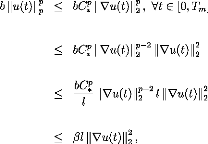
(3.18)

p-2

which means by the definition of l

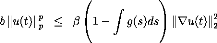
bb u(t)t)rp 0 0 1 1-- g(s)dsds) 1u(t)t)11

0

t
t

0 < 1--

1 g(s)ds A d1Vu(t)12212 Vt 2 E [0, Trri] .

where

. ·

(3.19

0

= bCbC_*^P 2p 2_l

(p (p 2)2l^E(0)0))

t

0 1

Therefore,

b Ilu(t)rp < bCf mvu(t)kp2 ,g, v 2 E [0, Tri] < bCfkru(t)kp~2 2 -IVu(t)k22)~ bCp l kru(t)kp~2 ~ 2 l kru(t)k2 2 / 0l0 IVu(t)k22)g tt 0 g(s)ds ds

_Z

0

I(t) = _@1 ~ g(s)ds _{d A}1Vu(t)k²₂)g + (g Vu)(t)t) -- b Ilu(t)r_p > 0. (3.20)

for all t 2 [0,T,] ,

By taking the fact that

p-2

lim ti-).7',7,

bCf, ( ^213 E (0)) 1 \03 -- 2) 1 j

2

< 0 < 1. (3.21)

This shows that the solution u(t) 2 W, for all t 2 [0, T_rn] . By repeating this procedure T_m extended to T.

Proof of Theorem 3.1.1.

In order to prove theorem 3.1.1, it suffices to show that the following norm

Ivu(t)I2 + 11⁷⁴(0112 , (3.22)

is bounded independently of t.

To achieve this, we use (3.4) , (3.14) and (3.15) to get

1

E(0) > E(t) = J(t) + ₂ Ilut(t)g

_{0 1 3}

p ~ 2 ~ 2 Zt

? 0

₄ @1 ~ g(s)ds A kru(t)k2 ₂ + (g ~ ru)(t) 5 2p

1 1

+₂ Mut(t)112 ² + _PI(t)

p ~ 2 ~ l kru(t)k2 ₂ + (g ~ ru)(t)~ + 1

? 2 kut(t)k2 ₂ + ¹ pI(t)

2p

(3.23)

~p ~ 2 ~ ~ ~

2 + 1

? l kru(t)k2 ₂ kut(t)k² ;

2

2p ⁾

since I(t) and (g o Vu)(t) are positive, hence

1vu(01²₂₂ + mut(t)k²₂g < CE(0),

where C is a positive constant depending only on p and 1. This completes the proof of theorem 3.1.1.

The following lemma is very useful

Lemma 3.1.5 ([44]) Suppose that (2.3) and (3.12) hold. Then

tb Ilu(t)r_p < (1 -- n) (1 -- I g (s)ds) kru(t)k² (3.24)

0

2

where n = 1 -- 0.

3.2 Decay of Solutions

We can now state the asymptotic behavior of the solution of (P).

Theorem 3.2.1 Suppose that (G1) , (G2) and (2.3) hold. Assume further that u0 2 W and ui 2 1¹₀ (Q) satisfying (3.12) . Then the global solution satisfies

E(t) < E (0) exp (--At) , Vt > 0 if m = 2, (3.25)

or

E(t) < (E(0)^' + Kort)³ , Vt > 0 if m > 2, (3.26)

where A and K0 are constants independent of t, r = m 1 and s =

2

2 2 -- m.

The following Lemma will play a decisive role in the proof of our result. The proof of this lemma was given in Nakao [34].

Lemma 3.2.1 ( [37]) Let cp(t) be a nonincreasing and nonnegative function defined on [0, T] , T > 1, satisfying

cp^l#177;r(t) < k( (cp (t) -- cp (t + 1)) , t 2 [0, T] ,

for ko > 1 and r > 0. Then we have, for each t 2 [0, T] ,

cp (t) < cp (0) exp (--k [t -- 1]⁺) , r = 0

c° (t) ~{c (0)^--r + k0r [t -- ¹]⁺1

{

_1 ^r ,r > 0

,

(3.27)

where [t -- 1]⁺ = max ft -- 1,0} , and k = ln ( k0 k0 1 ₁) .

Proof of Theorem 3.2.1.

Multiplying the first equation in (P), by ut and integrate over ft to obtain d dt E (t) + w 11out 1²2 + a Mud 2 : = (g' 2

Vu) (t) -- g (t) 11V u(t)11²₂

Then, integrate the last equality over [t, t + 1] to get

t+1 t+1

E(t 1) -- E(t) + w kbut1²₂ ds + a Mud: ds

t t

=

t+1

t

1 (g^' 0 V u) (s)ds --

²

t+1

₂g(s) 1Vu(t) 1 2ds

t

Therefore,

1

E(t) -- E(t 1) = fi^m(t) -- ₂

1

(g' o VU) (s)ds +

2

t+1

g(t) 1Vu(t)k²₂ ds, (3.28)

t

t+1

t

where

t+1 t+1

F^m(t) = a Mud: ds w 1Vutk²₂ ds (3.29)

t t

Using Poincaré's inequality to find

t+1 t+1

Iutk²₂ ds < C (12) Mutem ds (3.30)

t t

Exploiting Holder's inequality, we obtain

_{0 1}

_Zt + 1

kutk2 _m ds ~ @ ds _A

t

m-2

_m 0

@

₁

2

~kutk2 m A

m

t+1

t

t+1

t

2
m

ds

0 ~ @

t+1 t

1 2 ~kutk2 m A m

2 m

ds. (3.31)

Combining (3.29), (3.30), and (3.31), we obtain, for a constant C1, depending on ~

t+1

Iutk²₂ ds < F²(t), C1 > 0. (3.32)

t

~ ~

By applying the mean value theorem, ( Theorem 1.3.3. in chapter1), we get for some t1 2 t_; t + 1 ;

4

~ ~

t + 3

t2 2 _4; t + 1

Ilut(ti)112 < 2c (n)

1 ^2 F(t), = 1, 2. (3.33)

Hence, by (G2) and since

t+1

1Vut1²₂ ds < C2F (t)², C2 > 0 (3.34)

t

1 3

, there exist t1 2 [t' 4 t + 1 , 4 t2 2 [t + t + 11 such that

11Vut(ti)11²₂ < 4C (Q)F(t)², i = 1, 2. (3.35)

_Zt 2

tl

Next, we multiply the first equation in (P) by u and integrate over Q x [t1, t2] to obtain

_{2 0 1 3}

_Zt

_{4 @}1 ~ g(~)d~ _A kru(t)k2 ₂ ds ~ b kuk^p ₅ ds

0

p

= ~

Zt 2 tl

I

u.uttdxds -- w

Zt 2 tl

I

Vu.Vutdxds -- a

Zt 2 tl

Z

u: jutj^m-2utdxds

t2 +f tl

Zs 0

g(s ^-T) I

Vu(s). [Vu(T) -- Vu(s)] dxdrds.

Obviously, t 2 Z tl

I(s)ds = --

Zt 2 tl

Z

u.uttdxds -- w

Zt2 tl

Z

Vu.Vutdxds -- a

Zt 2 tl

Z

u.lutr^-2 utdxds

t 2 + f tl

Zs 0

g(s ^-T) I

Vu(s). [Vu(T) -- Vu(s)] dxdrds

~~~~~~

=

~~~~~~

u.uttdxds

~_~~Zt2

~~~

tl

I

_{2 3}

_{Z Z}t 2 _Z

₄ utudx ₅ ~ utdxds

t2

~ t1 t1 ~

=

~~~~~~

Z

ut(t2)u(t2)dx -- I ut(ti)u(ti)dx --

Zt 2 tl

kutk^2 2ds

~~~~~~

;

t 2

+ f (g o Vu) (s)ds. (3.36)

tl

Note that by integrating by parts, to obtain

Using Hölder's and Poincaré's inequalities, we get

~~~~~~

2

_Z

u.uttdxds

< C2 ~

_X
i=i

~_~~Zt 2

~~~

tl

1Vutk²₂ dt. (3.37)

Iout(ti)12 Ilvu(ti)112 + C2 ~ _Zt2

tl

By using Hölder's inequality once again, we have

~~~Zt 2 ~~~ tl

I

Vu.Vutdxds

~~~~~~

t2 I~ tl

1V7k2 1Vuth ds (3.38)

Furthermore, by (3.35) and (3.16), we have

1 1

kVtt(ti)1₂ 1Vt(ti)1₂ < C3 (C(Q)) 2 F(t) sup E(s) 2 ; (3.39)

h<s<t2

where, C3 = 2 (1 _(p ²--^p 2))

1

2

:

From (3.34) we have by Hölder's inequality

Zt 2 tl

1V7k2 1Vuth dt <

Zt 2 tl

E(s)

1 ~ 2p ~~ 1 2 l p ~ 2

1 2

11VUt112 ds

< 1 2C3 sup E(s) ti<8<t2

1 2

Zt 2 tl

1Vuth ds,

which implies

1

1

2

1 krutk2 ₂ dt _A

0

11Vut112 dt < _@1dt

_Zt2

tl

t1

₁

_A

t2

₂ 0

@

_Zt 2

tl

Then,

~~~Zt 2 ~~~ tl

Z

u.uttdxds

~~~~~~

< 2C^2~C3F(t) sup h<s<t2

1 E(s)^2 + C!C2F(t)^2. (3.41)

-- 2

N/3C2 F(t).

C3 3C2

where C4 =

4

1

E(s) 2 (3.40)

_Zt 2

tl

1Vu12 1Vuth dt < C4F(t) sup h<s<t2

. Therefore (3.37) , becomes

We then exploit Young's inequality to estimate

Zt 2 ,

I i st 0

g(s - r)Vu(t). [Vu(s) - Vu(t)1 drdxdt

(3.42)

< 8

Zt 2 h

t I 0

g(s - 7^-)11Vu11^22c/rdt+ 4^16.

, I h

(g o Vu) (t)dt, VS > 0.

Now, the third term in the right-hand side of (3.36), can be estimated as follows

Zt 2 h

t 2 f 17/11^m-2 ut.udxds < I ~ tl

I

lutl^m-1 . lul dads.

By Holder's inequality, we find

Zt 2 h

I

lutr^n-1 . lul dxds <

Zt 2 h

2 664

0 1 Z @jutj^m dx A ~

m1 m 0 1 Z @ juj^m dx A ~

3 ^1 ^m 5 7 7

ds

kutk

=

_Zt 2

h

^m~1 m ll'all_m ds.

By Sobolev-Poincare's inequality, we have

, I ti

kutk^m~1 m Mullm ds < C(S2)

Zt 2 ti

kutk^m~1 m 1Vu12 ds,

for 2 < m ~ 2n n - 2

if n > 3, or 2 < m < 1 if n = 1, 2.

Using Holder's inequality, and since ti, t2 2 [t, t + 1] and E(t) decreasing in time, we conclude from the last inequality, (3.16) and (3.29) , that

, I ti.

Ilut1C^-1 Mullm ds < C (Q) (l (p ^2--^p 2))

1 2

Zt 2 ti.

Ilut1C^-1 (J (u))^I2 - ds

< C (Q) (l (p ^2! 2))

1 2

Zt 2 ti

1 Ilut1C^-1 (E(u))^2 ds

1

< C (Q) (l (p ^2! 2))	2		(E(u))	1
		sup h<8<t2		2 x
0 Zt2 @t1					1 kutkm m ds A		m-1	0 Zt 2 @t1	1 ds A	1 M
											(3.43)

m-1 1

( 1a )

M

C (Q) sup h<8<t2

(E(t))

21 ( 2p ) l (p -- 2))

2

F (t)^m-1

Then, taking into account (3.41) -- (3.43), estimate (3.36) takes the form

_Zt 2

ti.

1

I(t)dt < (2C! + ^3C2 w) C3F(t) sup E(s)² + C:C2F(t)²

4 ti <8<t2

2 C3C (Q) sup (E(t))

1

₂ F(t)m-1

1

M

a

+

h<8<t2

(3.44)

+8

, I ti

t I 0

g(t -- s) 11V u112 dsdt + (1 48 + 1)

, I h

(g 0 Vu) (t)dt.

Moreover, from (3.4) and (3.10), we see that

E(t) = 2 kutk2

1 2 dt + J(t)

t

=

2 2p

1 Ilutg + (p 2) 1 -- I g(s)ds) 11V u112

0

(3.45)

1p 2p-- 2 \

+ ) (g 0 Vu) (t) + ¹ I (t).

By integrating (3.45) over [t1, t2] , we obtain

, I ,

E(t)dt = 1 2

Zt 2 h

11utg dt + 132p2/

, I ,

0 @1 --

t I 0

1 g(s)ds A 11Vu11^22 dt

+ (p -- 2) 2p

Zt 2 ,

(g o Vu)(t)dt + 1 P

Zt 2 ,

I(t)dt, (3.46)

which implies by exploiting (3.32)

t 2 I .

E(t)dt < c 1 (F (t))^2 + 2 1 P

Zt 2 ,

/(t)dt + (P -- 2) 2p

Zt 2 ,

(g o Vu) (t)dt

(3.47)

+ (p -- 2) 2p

Zt 2 h

0 @1 --

t I 0

1 g(s)ds A 11Vu11^22 dt.

By using (3.11), Lemma 3.1.5, we see that

0 @1 --

t I 0

)

g(s)ds 11V ug < ¹1(t). (3.48)

⁷1

Therefore, (3.47), takes the form

t 2 I

Q)( E(t)dt < C 2 (F(t))^2 + (P -- 2) 2p

, I ,

(g o Vu) (t)dt

+ (1 + p -- 2) .75, 2pii )

Zt 2 ,

I(t)dt. (3.49)

Again an integration of (3.14) over [s, t2] , s E [0, t2] gives

E(s) = E(t2) + a

Zt 2 8

1 11ut(t)11: dr + 2

, I 8

g(T) 11Vu(t)11^22 dr

--

1 2

Zt 2 8

(g o Vu) (t)dr + w

Zt 2 8

11Vut(t)11^22 dr (3.50)

Zt 2 ,

E(s)ds >

t 2 I

1 E(t2)ds > 2E(t2) · (3.51)

1

'

By using the fact that t2 -- ti > 2 we have

The fourth term in (3.44), can be handled as

t I 0

g(t -- s) 1Vu1^22 ds = 1Vu1^22

t I 0

g(t -- s)ds

(3.52)

< 2p (1 -- l) E (t). -- l (p -- 2)

Thus,

t2 I t1

t I 0

g(t -- s) 1Vuk^22 dsdt < 2p (1 ~ l) l (p -- 2)

t2 I t1

E(t)dt

p (1 ~ l)

~ l (p -- 2)E(ti)

~ p (1 ~ l) l (p -- ₂₎E(t). (3.53)

Hence, by (3.53) , we obtain from (3.44)

t2

_I

t1

1

I(t)dt < ( 20, + ^3C2w) C3F(t) sup E(s)² + C!C2F(t)²

4 ti<8<t2

2 C3C (Q) sup (E(t))

1

₂ F(t)m-1

1

m

a

+

ti<8<t2

E(t) + ( 1 + 1) +8 l (p -- 2) 48

t2 I t1

(g o Vu) (t)dt. (3.54)

E(t) < 2

t2 I t1

E(s)ds + a

t + 1 I t

1 Iut(t)1^mm dr + 2

t + 1 I t

g(r) 1Vu(t)k^22 dr

~

1 2

t + 1 I t

(g^' o Vu) (t)dr + w

t + 1 I t

1Vut(t)k^22 dr. (3.55)

From (3.50) and (3.51) we have

Obviously, (3.49) and (3.55) give us

( c (Q) )

f /(t)dt E(t) < 2 (F(t))² + (P 2 ² ) t 2 t 2

I (g ° Vu) (t)dt + (¹ + p -- 2)

2 p 2pn

tl tl

+a

Zt 2 ,

1 kut(t)km m dt + 2

, I ,

g (t) 11V u(t)g dt -- 12

, I ,

(g^' o Vu) (t)dt

_Zt 2

,

+w

1Vut(t)k²₂ dt.

Consequently, plugging the estimate (3.54) into the above estimate, we conclude

E(t) < C (Q) (F(t))^2 + (P 2) P

, I ,

(g o Vu) (t)dt

.V3C2 1

+2 1¹ + P-- ²) [(2C: + ₄ w) C3F(t) sup E(s) 2 + C!C2F(t)²1

P 2pn ti<8<t2

+

(1 + P 2) _am¹ C3C (Q) sup (E(t)) ² F(t)^m-1 p 2pi
t

i

<

8

<t2

+2 (1 p + 2pn p -- 2) [Sp1 (p -- 2) E (t) + (_4S + 1 ) I (g 0 V u) (t)dt)1

1

l

t

t2

(3.56)

+F^m(t) -- 1 2

, I ,

(g^' o Vu) (t)dt + 2

, I ,

g (t) 11V u(t)g dt.

We also have, by the Poincaré's inequality

I I u(s) I I 2 < C I I vu(s)II2

1

< C (1 (p --^p 2))

2

E(t)

1 2

, (3.57)

Choosing 8 small enough so that

1 -- 2 (¹ + p -- 2) _Sp (1 -- 1)

(3.58)

p 2pi 1 (p -- 2) > 0'

we deduce, from (3.56) that there exists K > 0 such that

E(t) < K [ F(t)² + E(t) 2 F(t) + E(t) 2 F(t)^m-1 + F(t)^m_]

+

1 2

t + 1 I t

g(s) 1Vu(s)k^22 ds -- 1 2

t + 1 I t

(g^' o Vu) (s)ds

(3.59)

#177;[(p ;2) #177; 2 ( 15. #177; 0 (p i_ #177; p 2-13712)1

t + 1 I t

(g o Vu) (s)ds

,

_I

,

Using (G2) again we can write

, I ,

(g o Vu) (t)dt < --

(g^' 0 Vu) (t)dt, > 0.

Then, we obtain, from (3.59),

1 1 ,

E(t) < K [ F(t)² + E(t) ² F(t) + E(t) ² F(t)^m-1 + F(t)^m_]

(3.60)

g(s)11Vu(s)gds -- ( 6+ 2)

1

+ 2

t + 1

_I

t

t + 1

_I

t

(g^' o Vu) (s)ds.

where 6_. = [(p ;2) + 2 (_.731 #177; p 2p--n) ( 45+ 1 )J

An appropriate use of Young's inequality in (3.60), we can find K1 > 0 such that

E(t) < K1 [F(t)² + F(t)^2(m-1) + F(t)^m] (3.61)

g(s)11Vu(s)gds -- ( 6+ 2)

₃

(g^' o Vu) (s)ds 5 ,

t + 1

_I

t

t + 1

_I

t

[

1

2

for K1 a positive constant.

Using (G2) again to get

E(t) < K1 [F(t)² + F(t)^2(m-1) + F(t)^m]

+ [ (1 + 2 f

g (s) 11V u(s) g ds -- (61 + 2)

t + 1

_I

t

t+ 1

_I

t

(g^' o Vu) (s)ds

< K1 [F(t)² + F(t)^2(m-1) + F(t)^m]

(3.62)

t + 1 t + 1

+ (1 + gi)

[2

1 I

I g(s) 11V u(s)112 ² 2 ds -- (g^' o Vu) (s)ds

t t

At this end we distinguish two cases:

Case 1. m = 2. In this case we use (3.28) and (3.62), we can find K2 > 0 such that

E(t) < K1 F(t)²

t+ 1 t + 1

+ (1 + gi)

[2

I g(s) 11V u(s)11₂ ds -- 2 II (g^' o Vu) (s)ds

t 1

t

< K2 [E(t) -- E(t + 1)] . (3.63)

Since E(t) is nonincreasing and nonnegative function, an application of Lemma 3.2.1 yields

E(t) < K2 [E(t) -- E(t + 1)] , t > 0, (3.64)

which implies that

E(t) < E (0) exp (--A [t -- 1]1 , on [0, oo) , (3.65)

where A = ln

K2 -- 1

( K2

Case 2. m > 2. In this case we, again use (3.28) and (3.62) to arrive at

2

m

. (3.66)

t + 1 t+ 1t t

F(t)² = (E(t) -- E(t + 1)) -- 2 1 I g(s) 11V u(s) g ds + 21 I (g^' o Vu) (s)ds

m

2 < 2

We then use the algebraic inequality

(a + b)

m ( m m

2 _a2 + b²), m > 2. (3.67)

To infer from (3.62), and by using (3.67), that

[E(t)]

m [1 + F (t)^2(m_2) + F (t)^m_2] 2 < K3

m 2 F(t)m

	m 2 (1 + 21)	m	2 4	ft + 1 1 g(s) MVu(s)M2 2 ds _ 1 2 2 t	Zt + 1 t	3 (g^' o Vu) (s)ds 5		m 2	+2

[1 + F (t)^2(m_2) + F (t)^m_2]^m

< K3 2 x [E(t) - E(t + 1)]

(3.68)

	m 2 (1 + 21)	m	2 4	ft + 1 1 g(s) MVu(s)M2 2 ds _ 1 2 2 t	Zt + 1 t	3 (g^' o Vu) (s)ds 5		m 2	+2

m

where K3 = 2

2 K1. We use (3.28) to obtain

0 @

1 2

Zt + 1 t

g(s) VuM2 2 ds - 1 2

Zt + 1 t

1 (g^' o Vu) (s)ds A

m 2

m

< (E(t) - E(t + 1)) A combination of (3.68), (3.69) yields

2 (3.69)

[E(t)]

m 2 < K3 [1 + F(t)^2(m_2) + F(t)^m_2]

m 2 x (E(t) - E(t + 1))

+2

m 2 (1 + 21)

m 2 [E(t) -- E(t + 1)]

m 2 -1 [E(t) - E(t + 1)]

[ ]

m m m

< K3 [1 + F (t)^2(m_2) + F (t)m_2]m ² + 2 2 ~1

2 (1 + 21) ² [E(t) - E(t + 1)] x

[E(t) - E(t + 1)] (3.70)

By using (3.62), the estimate (3.70) takes the form

[E(t)]

m 2 <

{ m m m m K32m [1 + E(0)^(m_2) + (E(0)) 2 ~1i 2 _1} + 2 ^2 (1 + 21) ^2 (E(0)) ~

(E(t) - E(t + 1))

< K0 (E(t) - E(t + 1)). (3.71)

Again, using Lemma 3.2.1, we conclude

E(t) < [E(0)_^r + K0r [t -- 11⁺1⁸ , (3.72)

Tn

with r =

2

2

1 > 0, s = and K0 is some given positive constant.

2 -- n-i

This completes the proof.

Chapter 4

Exponential Growth

Abstract

_f

⁰⁰ g(s)ds < p -- 2

p -- ₁, by

0

Our goal in this chapter is to prove that when the initial energy is negative and p > m, then, the

solution with the L^u--norm g

rows as an exponential function provided that

using carefully the arguments of the method used in [16], with necessary modification imposed by the nature of our problem.

4.1 Growth result

Our result reads as follows.

Theorem 4.1.1 Suppose that m > 2 and m < p < oo, if n = 1,2, m < p < 2 (n -- 1) if n > 3.

n -- 2 --

p -- 2

00

holds. Then the unique local solution of problem

Assume further that E(0) < 0 and f g(s)ds <

0 p --1

(P) grows exponentially.

Proof. We set

H(t) = --E(t). (4.1)

By multiplying the first equations in (P) by --ut, integrating over Q and using Lemma 2.1.3, we obtain

t

₈

<

:

d

~ dt

_{0 1 9}

_Z =

2 kutk2

1 2 + 1 _@1 ~ 2 + 1

g(s)ds _A kruk2 ₂ (g ~ ru) (t) ~ p b kukp p

2 ;

0

1

1

= a IlutIC -- 2 (g' _o Vu)(t) + ₂ g(t) 11V ug + w rout g .

(4.2)

By the definition of H(t), (4.2) rewritten as

1

H'(t) = a Mutr_m -- 2 2 (g^' o Vu) (t) + ¹ g (t) 11V 74²₂ + w 1out1²₂ > 0, Vt > 0. (4.3)

Consequently, E(0) < 0, we have

1 2 + b

H(0) = ~₂ ku1k2 ₂ ~ 2 1 kru0k² _pMuce_p > 0. (4.4)

It's clear that by (4.1), we have

H(0) < H(t), Vt > 0. (4.5)

Using (G2) , to get H(t) -- b p One implies		2 0 1 3 Zt kukp 41 p = ~ 2 kutk2 2 + 1 @1 ~ g(s)ds A kruk2 2 + 2 1 (g ~ ru) (t) 5 2 0 < 0, Vt > 0. (4.6)		0 < H(0) < H(t) < b p
Iul^Pp . (4.7)

Let us define the functional

L(t) = H(t) + E./ n

ii ii 2 utudx + E 2 w IIVu112 . (4.8)

for E small to be chosen later.

By taking the time derivative of (4.8) , we obtain

L^'(t) = H^'(t) + E./ n

uutt (t, x)dx + F E 1lutg + Ew I SI

VutVudx

= [wIlVutg + a IlutI^m_m - ₂ (g^' o Vu) (t) + ¹₂g(t) 11V ug]

+E 1lutg + Ew I n Using the first equations in (P), to obtain

VutVudx + E I n

uttudx. (4.9)

Iuuttdx = bllurp HIV ug - col ~

VutVudx - a f n

1ut1^m-2 utudx

+I n

Vu

t I 0

g(t - s)Vu(s, x)dsdx. (4.10)

Inserting (4.10) into (4.9) to get

1

L^'(t) = wIlVutg + a MutE_r^m_i -₂ (g^' o Vu) (t) + ¹ 2g(t)1Vuk22

+ E Iutl22 --E 1Vuk^22 + E

t I 0

g(t - s) f Vu.Vu(s)dxds

+ EbIlurp - Ea I n

lutr^m-2 utudx. (4.11)

By using (G2) , the last equality takes the form

L^'(t) > w 1Vutk²₂ + a Iutr^m_m + E Iutk²₂ -E 1Vuk²₂ +EbIlur_p

(4.12)

+E

t I 0

g(t - s) f Vu.Vu(s)dxds - Ea f ~ n

lutr^m-2 utudo^-.

To estimate the last term in the right-hand side of (4.12) , we use the following Young's inequality

r XY < r

Xr + 8-q q

Y ^q, X, Y > 0, (4.13)

for all 8 > 0 be chosen later, 1 r So we have

+

1 q

m = 1, with r = m and q = m _ 1.

I

lutr^n-2 utudx <

I n

lutr^n-1 lul dx

MuM: + (mm 1) 8(m71) IlutIC , Vt > 0. (4.14)

8^m

<

m

Therefore, the estimate (4.12) takes the form

L^'(t) > w 11Vut11²2+ a Ilutr,,+E Mut11²2 ^-E 11Vu11²2+EbIlurp

t

_I

0

+ E

g(t - s) I Vu.Vu(s)dxds

E8^m a m

Murn^i Ea (m m 1) 8(mi^ni) 11u4117,

> w Ivutk22 + a IlutIC + E Iutk22 -- E 1Vuk²₂ + Eb 1uk1p

+ E r uk^22		t I 0	g(s)ds + E	t I 0	g(t - s) I Vu (t) [Vu (s) - Vu (t)] dxds
8 Ea^ln m	NC Ea (m m1) 8(^mm) IlutIC . (4.15)

Using Cauchy-Schwarz and Young's inequalities to obtain

L^' (t) > w 11V utg + a ( 1 - E ( ^{7 1} ₇₇^-₁¹) gmln1)) IlutIC + E 1lutg

E 1Vuk22 + Eb bun + E r uk^22

t I 0

g(s)ds

t

_I

0

E

Mull:

g(t - s) 11V u112 11V u(s) - Vu _(t)112 ds -- Ea^rl

m

> w 11V utg + a ( 1 -E (m m1) gm^ln1)) 11utr_nⁱ + E Ilutg + Eb Ng

(4.16)

₀

+ E @

1 2

t I 0

)g(s)ds -1 11V ug - E2 (g o V u(t) - Ea: Mull: .

Using assumptions to substitute for b Ilur_p . Hence, (4.16) becomes

L^'(t) > w IlVut11₂ + a ( 1 -- E (M m1) 8( min1)) Mud: + EllUt112

-FE (311(t) #177; 2 Ilutg + 2 (g 0 Vu) (t) + ^P₂ 1 -- I g(s)ds 11Vug

0t

1

2

-FE

t

_I

0

)

m

g(s)ds --1 11Vug -- E₂ (g o Vu(t) --ga_m Mull: .

> w 11Vutg + a ( 1 --E (m m -- ₁₎ 8( 7/7-)11 )) 11utr,,+ E (1 + 2) 1lUtg

(4.17)

+EallIVug + Ea2(9 0 Vu(t) -- Ea^ri Mur_rⁿ_i + €pH(t).

m

(1 --

f g(s)ds #177; ( P

where al = ) > 0, a2 = P 1 > 0.

0

2 p ) 22 2

In order to undervalue L^'(t) with terms of E(t) and since p > m, we have from the embedding L^P (Q) c-- L^m (Q) ,

m

Mur_rⁿ_i < C Ilugⁿ, < C (Ilur_p) P , Vt > 0. (4.18)

for some positive constant C depending on Q only. Since 0 < m P

< 1, we use the algebraic inequality

Zk < (Z #177; 1) < ( 1 #177; 1 ) (Z #177; W) , V Z > 0, 0 < k <1, w > 0, w

to find		m		(Mull;)
^P < K (Ng + 11(0)) , Vt > 0, (4.19)

1

0)

where K = 1 + H( > 0, then by (4.7) we have

IluEⁿ_i < C ( 1 + b) Mug, Vt > 0. (4.20)

P

Inserting (4.20) into (4.17), to get

L^'(t) > w IlVutg + a ( 1 -- E (m m - ₁₎ 8( ⁷¹⁷¹⁾) IlUtIr_m^l + E (1 + 2) 1lUtg

(4.21)

-Ec1 1Vuk22 + Ea2(9 ⁰ Vu(t) -- EC1114¹³_p#177; €pH(t).

where Ci = aC r771 ( 1 + b) > 0.

p

By using (4.1) and by the same statements as in [16], we have

2H(t) = - Iutl22 -^Ivuk22 +

Zt 0

g(s)ds kruk2 2 ~ (g ~ ru) (t) + 2b p

Ilull^Pp

(4.22)

~ ~Iutk²₂ IVuk²₂ -- (g Vu) (t) + 2pb Mur_p , Vt > 0.

Adding and substituting the value 2a3H(t) from (4.21), and choosing 8 small enough such that

a3 < min {al, a2} , we obtain

L^'(t) > w _Iloutll2 + a (1 -- E (m m1) 8 ( mln1)) Ilutrrni

+ E 11 + 2 -- a3) Iutk²₂ + E (al a3)1Vuk²₂

+ E (a2 -- a3) (g _o Vu(t) + E (2p ^b a3 -- C1) 1uk¹_p

+ E (p -- 2a3) H(t). (4.23)
Now, once 8 is fixed, we can choose E small enough such that

1 -- E (m m1) g^mlni) > 0, and L(0) > 0. (4.24)

Therefore, (4.23) takes the form

L^'(t) > E0 {H(t) + Ilutg+ I1Vug+ (g o Vu(t)) + Mur_p} , (4.25)

for some 0 > 0.

Now, using (G2), Young's and Poincare's inequalities in (4.8) to get

L(t) < 01 {H(t) + _11741122 + IlVu112 2},(4.26) for some 01 > 0. Since, H(t) > 0, we have from (4.1)

t

1

2 ^mutg 2 -10 1- f g(s)ds) 11V 2

-- (g _o Vu) (t)+bIIuIIP > 0, Vt > 0. (4.27)

0

Then,

1 2

0 @1 --

Zt 0

g(s)ds) Iloull2 < p b Murp

b
p

<

Mur_p + (g _o Vu) (t). (4.28)

In the other hand, using (G1) , to get

1 1

2 (1 -- l)11V ug 2

< (1 t

-- I g(s)ds) 11V ug

o

b

<

p

11u11^p_p + (g 0 Vu) (t). (4.29)

Consequently,

2b 11Vug < p

11u11^pp + 2 (g 0 Vu)(t) + 2l 11Vu11^22 , b,l > 0. (4.30)

Inserting (4.30) into (4.26) , to see that there exists a positive constant A such that

L(t) < A { H(t)+ 11ut11²₂+11Vu11²₂+ (g 0 Vu)(t)+ bp 11ur_p} , Vt > 0. (4.31)
From inequalities (4.25) and (4.31) we obtain the differential inequality

L'(t)

> it, for some ,u > 0, Vt > 0. (4.32)
L(t)

Integration of (4.32) , between 0 and t gives us

L(t) > L(0) exp (itt) , Vt > 0, (4.33)

From (4.8) and for E small enough, we have

By (4.33) and (4.34) , we have

L(t) < H(t) < b p

11u11^Pp . (4.34)

11u11^p_p > C exp (ut), C > 0, Vt > 0. (4.35)

Therefore, we conclude that the solution in the L^P--norm growths exponentially.

Bibliography

[1] J. Ball, Remarks on blow up and nonexistence theorems for nonlinear evolutions equations, Quart. J. Math. Oxford, (2) 28, 473-486, (1977).

[2] S. Berrimi and S. Messaoudi, Exponential decay of solutions to a viscoelastic equation with nonlinear localized damping, Electronic journal of differential equations, 88, 1-10, (2004).

[3] S. Berrimi and S. Messaoudi, Existence and decay of solutions of a viscoelastic equation with a nonlinear source, Nonlinear analysis, 64, 2314-2331, ( 2006).

[4] H. Brézis, "Analyse Fonctionnelle- Theorie et applications," Dunod, Paris (1999).

[5] M. M. Cavalcanti, V. N. D. Calvalcanti and J. A. Soriano, Exponential decay for the solutions of semilinear viscoelastic wave equations with localized damping, Electronic journal of differential equations, 44, 1-44, (2002).

[6] M. M. Cavalcanti and H. P. Oquendo, Frictional versus viscoelastic damping in a semi-linear wave equation, SIAM journal on control and optimization, 42(4), 1310-1324, (200).

[7] M. M. Cavalcanti, D. Cavalcanti V. N and J. Ferreira, Existence and uniform decay for nonlinear viscoelastic equation with strong damping, Math. Meth. Appl. Sci, 24, 1043-1053, (2001).

[8] M. M. Cavalcanti, D. Cavalcanti V. N, P. J. S. Filho and J. A. Soriano, Existence and uniform decay rates for viscoelastic problems with nonlinear boundary damping, Differential and integral equations, 14(1), 85-116, (2001).

[9] T. Cazenave and A. Hareaux, Introduction aux Problems d'évolution semi-linéaires, Ellipses, societe de mathematiques appliquees et industrielles.

[10] A. D. D and Dinh APN, Strong solutions of quasilinear wave equation with nonlinear damping, SIAM. J. Math. Anal, 19, 337-347, (1988).

[11] C. M. Dafermos and J. A. Nohel, Energy methods for nonlinear hyperbolic volterra integrodifferential equations, Partial differential equations, 4(3), 219-278, (1979).

[12] C. M. Dafermos, Asymptotic stability in viscoelasticity, Arch. Rational Mech. Anal, 37 1970 297-308.

[13] F. Gazzola and M. Sequassina, Global solution and finite time blow up for damped semi-linear wave equation, Ann. I. H. Pointcaré-An 23 185-207, (2006).

[14] V. Georgiev and G. Todorova, Existence of solution of the wave equation with nonlinear damping and source terms, Journal of differential equations 109, 295-308, (1994).

[15] S. Gerbi and B. Said-Houari, Local existence and exponential growth for a semilinear damped wave equation with dynamic boundary conditions, Advances in Differential Equations, July 2008.

[16] S. Gerbi and B. Said-Houari, Exponential decay for solutions to semilinear wave equation, submitted.

[17] A. Haraux and E. Zuazua, Decay estimates for some semilinear damped hyperbolic problems, Arch. Rational Mech. Anal, 150, 191-206, (1988).

[18] W. J. Hrusa and M. Renardy, A model equation for viscoelasticity with a strongly singular kernel, SIAM J. Math. Anal, Vol. 19, No 2, March (1988).

[19] R. Ikehata, Some remarks on the wave equations with nonlinear damping and source terms, Nonlinear Analysis. Vol 27, no 10,1165-1175, (1996).

[20] V. K. Kalantarov and Ladyzhenskaya O. A, The occurrence of collapse for quasilinear equation of parabolic and hyperbolic type, J. Soviet Math, 10, 53-70, (1978).

[21] M. Kopackova, Remarks on bounded solutions of a semilinear dissipative hyperbolic equation, Comment Math. Univ. Carolin, 30(4), 713-719, (1989).

[22] Levine H. A and S. Park. Ro, Global existence and global nonexistence of solutions of the Cauchy problem for nonlinear damped wave equation, J. Math. Anal. Appl, 228, 181-205, (1998).

[23] H. A. Levine, Instability and nonexistence of global solutions of nonlinear wave equation of the form Putt = Au + F(u), Trans. Amer. Math. Sci, 192, 1-21, (1974).

[24] H. A. Levine, Some additional remarks on the nonexistence of global solutions of nonlinear wave equation, SIAM J. Math. Anal, 5, 138-146, (1974).

[25] H. A. Levine and J. Serrin, A global nonexistence theorem for quasilinear evolution equation with dissipative, Arch. Rational Mech Anal, 137, 341-361, (1997).

[26] J. L. Lions, "quelques méthodes de résolution des problemes aux limites non lineaires," Dunod, Gaulthier-Villars, Paris (1969).

[27] J. L. Lions, "Controle optimal de systemes gouvernés par des équations aux dérivées partielles," Dunod, Gaulthier-Villars, Paris (1968).

[28] Z. Liu and S. Zheng, On the exponential stability of linear viscoelasticity and thermoviscoelasticity, Quarterly of applied mathematics. Vol LIV, number 1, March, 21-31, (1996).

[29] S. Messaoudi, Blow up and global existence in a nonlinear viscoelastic wave equation, Maths Nachr, 260, 58-66, ( 2003).

[30] S. Messaoudi, On the control of solution of a viscoelastic equation, Journal of the ranklin Institute 344 765-776, (2007).

[31] S. Messaoudi, Blow up of positive-initial energy solutions of a nonlinear viscoelastic hyperbolic equation, J. Math. Anal. Appl, 320, 902-915, (2006).

[32] S. Messaoudi and B. Said-Houari, Global nonexistence of solutions of a class of wave equations with nonlinear damping and source terms, Math. Meth. Appl. Sc, 27, 1687-1696, (2004).

[33] S. Messaoudi and N-E. Tatar, Global existence and asymptotic behavior for a nonlinear viscoelastic problem, Mathematical. Sciences research journal, 7(4), 136-149, (2003).

[34] S. Messaoudi and N-E. Tatar, Global existence and uniform stability of a solutions for quasilinear viscoelastic problem, Math. Meth. Appl. Sci, 30, 665-680, (2007).

[35] S. Messaoudi, Blow up in a nonlinearly damped wave equation, Math. Nachr, 231, 1-7, (2001).

[36] J. E. Munoz Rivera and M.G. Naso, On the decay of the energy for systems with memory and indefinite dissipation, Asymptote. anal. 49 (34) (2006), pp. 189204.

[37] M. Nakao, Asymptotic stability of the bounded or almost periodic solution of the wave equation with nonlinear dissipative term, J. Math. Anal. Appl, 56, 336-343, (1977).

[38] Vi. Pata, Exponential stability in viscoelasticity, Quarterly of applied mathematics volume LXIV, number 3, 499-513, September (2006).

[39] J. Peter. Olver, Ch. Shakiban, "Applied Mathematics," University of Minnesota, (2003).

[40] J. E. M. Rivera and E. C. Lapa and R. K. Barreto, Decay rates for viscoelastic plates with memory, Journal of elasticity 44: 61-87, (1996).

[41] J. E. M. Rivera and R. K. Barreto, Decay rates of solutions to thermoviscoelastic plates with memory, IMA journal of applied mathematics, 60, 263-283, (1998).

[42] B. Said-Houari, "Etude de l'interaction enter un terme dissipatif et un terme d'explosion pour un probleme hyperbolique," Memoire de magister ( 2002), Université de Annaba.

[43] R. E. Showalter, "Monotone Operators in Banach Space and Nonlinear Partial Differential Equation," By the American Mathematical Society, (1997).

[44] Shun-Tang Wu and Long-Yi Tsai, On global existence and blow-up of solutions or an integro-differential equation with strong damping, Taiwanese journal of mathematics.é.979- 1014, (2006).

[45] G. Teshl, "Nonlinear Functional Analysis," Universitat Wien, (2001).

[46] G. Todorova, Stable and unstable sets for the Cauchy problem for a nonlinear wave with nonlinear damping and source terms, J. Math. Anal. Appl, 239, 213-226, (1999).

[47] E. Vittilaro, Global nonexistence theorems for a class of evolution equations with dissipation, Arch. Rational Mech. Anal, 149, 155-182, (1999).

[48] W. Walter, "Ordinary Differential Equations," Springer-Verlage, New York, Inc, (1998).

[49] E. Zuazua, Exponential decay for the semilinear wave equation with locally distributed damping, Comm. PDE, 15, 205-235, (1990).