|
|
X Non Confidential ? Confidential
|
|
|
Title : Using the WACC Methodology to Improve
the
Assessment of Projects in the French Farming
Industry. Empirical Evidences from Farm's
Results
of Isère
Program: MBA - PT 6 - Grenoble (2009 - 2012)
Academic Year: 2011-2012
Dissertation / Project / Internship Report:
International Management Project 2011-2012 Student Name:
Bibard Anaël
School Tutor / Evaluator Name: Lominadze
Anton
To fill in for Internship only:
Company Name:
Town:
Country:
Position occupied during internship:
Summary: The Purpose of this Thesis is to
calculate the cost of capital for a typical farm in Isère. This cost of
capital is use as an actualization rate to estimate the NPV of projects or the
value of a farm based on this profitability.
Keywords:
https://library.grenoble-em.com/Thesaurus/Thesaurus.html
CORPORATE FINANCE - INVESTMENT
COMPANY - AGRICULTURAL COMPANY
ACCOUNTING - EVALUATION OF A COMPANY
FRENCH REGION - RHONE ALPES
MBA PT 6 - Grenoble Graduate School of Business
Using the WACC Methodology to
Improve the Assessment of Projects
in the French Farming Industry
Empirical Evidences from Farm's Results of
Isère
Anaël BIBARD
30/09/2012
Final Management Project Tutor: Anton Lominadze
Table of Content
Abstract 6
Abbreviations 7
Table of Illustrations 8
Introduction 11
1 Significance of the Research 12
1.1 The Farming Business in France 13
1.2 The Profitability Heavily Relies on Subsidies, Not on
Investment Decision 14
1.3 A New Approach to Find 17
2 Literature Review 20
2.1 Risk 20
2.1.1 Risk in Agriculture 20
2.1.2 Risk Premium 20
2.2 The WACC Theory 25
2.2.1 The Importance of the WACC Theory. 25
2.2.2 The Betas for Micro-Capitalizations 25
2.3 Discount Rates and the CAPM Used in Agriculture 26
3 Research Methodology 28
3.1 Survey Construction 28
3.1.1 Questionnaire 28
3.1.2 Results Analysis 28
3.2 Historical Analysis of the Results of Farms in Isère
28
3.2.1 Data Collection 28
3.2.2 Data Processing 30
3.2.3 Research Questions 31
3.2.4 Data Analysis 31
3.3 Bond Yield Plus Risk Premium Model 33
3.3.1 Risk-Free Rate 33
3.3.2 Beta and Risk premium 33
3.4 WACC Estimation 34
4 Data Analysis 36
4.1 Results of the Survey 36
4.2 Calculation of the Historical Results Using the Data from
CERFRANCE Isère 38
4.2.1 Normality of the Datasets 38
4.2.2 ROE 39
4.2.3 ROA 44
4.3 Calculation of the Capitalization Rate Using Bond Yields Plus
Risk Premium 49
4.4 Approach of the WACC for Farming in Isère 50
4.4.1 Calculation of the Betas 50
4.4.2 Calculation of the WACC for the Different Specialization
52
5 Discussion 55
5.1 Survey Results 55
5.2 ROE and ROA Analysis the Farms of Isère 55
5.3 Capitalization Using the Bond Yield Plus Risk Premium 56
5.4 The WACC Methodology 56
6 Utilization of These Results 58
6.1 Managerial Implications 58
6.2 Agricultural Policies Implications 59
7 Limitations and Further Research Implications 61
7.1 Survey Construction 61
7.2 ROE and ROA Analysis 61
7.3 Bond Yield Plus risk Premium Model 61
7.4 The WACC Methodology 62
7.5 Further Research Implications 62
Conclusion 63
Bibliography 64
Appendices 70
Abstract
The remarkable rise of the soft commodities prices in
2007/2008 represented just a reminder of the importance of agriculture for
humanity. The Arab spring found its base on this mold and pulled down many
regimes considered as stable few months before, like Tunisia or Egypt.
Eventually, these price records could be reached again in 2012, due to a severe
drought in the USA. To meet the challenge of feeding the world while developing
more sustainable forms of production, advisory services must play a great role
to help farmers in their decisions regarding their production as well as their
investments. However, it appears that some financial consultants use really low
actualization rates for agriculture, even lower than the risk-free rate. The
purpose of this paper is therefore to present the different methods that could
be used to determine more appropriate discount rates for farming businesses,
and particularly the Weighted Average Cost of Capital and the bond yield plus
risk premium model as presented by the French tax authority.
Historical results of farms from Isère over 5 years
were studied to determine if the leverage has a significant impact on the
profitability, and if signs of financial distress could be identified for the
higher leverages. The statistical tests performed confirmed the underlying
hypothesis of the WACC theory: the cost of capital is reduced by the increase
of the leverage, up to a limit where financial distress overcomes the advantage
of the lower cost of debt. The optimal capital structure for farms of
Isère seems to range between 40-60% leverage, and up to 60-80% in the
cases of the most stable production such as dairy farms.
This paper provides indications about how to establish the
actualization rates for agricultural consultants, based on the WACC methodology
and the method recommended by the tax authorities. The data analysis confirmed
that the actual rates used by practitioners are clearly undervalued, leading to
an over-valuation by two to four times in their asset valuation studies. The
WACC and the bond yield plus risk premium methodology both seem to be
applicable for small and medium farming businesses. However, further researches
are necessary to validate the robustness of the WACC methodology in the
agricultural context for non listed companies.
Abbreviations
ANOVA: Analysis Of Variance
CAP: Common Agricultural Policy
CAPM: Capital Asset Pricing Model
CNCER: Conseil National des CERFRANCE (national council of the
CERFRANCE) EBITDA: Earnings Before Interest, Taxes, Depreciation and
Amortization
EEP: Expected Equity Premium
FADN: Farm Accountancy Data Network, or RICA: Réseau
d'Information Comptable Agricole FAO: Food and Agriculture Organization
FTE: Full-Time Equivalent
GDP: Gross Domestic Product
Ha: hectare, 10 000 m2 or 2.47105 acres
HEP: Historical Equity Premium
IEP: Implied Equity Premium
IMF: International Monetary Fund
NPV: Net Present Value
NSP: Ne Se prononce Pas (No Answer)
OECD: Organization for Economic Cooperation and Development REP:
Required Equity Premium
ROA: Return On Asset
ROE: Return On Equity
SAFER: Société d'Aménagement Foncier et
d'Etablissement Rural SAS: Statistical Analysis System
SMIC: Salaire Minimum Interprofessionnel de Croissance. The
minimum salary in France. SPSS: Statistical Package for the Social Sciences
TCA: Total Cultivated Area
USD: US dollars
WACC: Weighted Average Cost of Capital
WTO: World Trade Organization
Table of Illustrations
Table 1: Subsidies and recurring net profit before tax in
France per farm, in K€Source: FADN (RICA) 16 Table 2: Assumptions and
recommendations of the 129 books that assume that REP = EEP. Source:
Fernandez 2010 21
Table 3: Equity premiums recommended and used in textbooks.
Source: Fernandez 2010 22
Table 4: Historical Equity Premium for the French market 23
Table 5: Historical Equity Premium for small and micro-cap 24
Table 6: Market capitalization effect on the beta for
micro-capitalization 26
Table 7: Primary data for the analysis of farms' results in
Isère 29
Table 8: Cost of each labor unit per month for the SMIC 30
Table 9: Social security contributions 31
Table 10: Groups of debt level 32
Table 11: Number of companies studied for the Beta estimation.
Source: Bloomberg 35
Table 12: Age and gender of the respondents 36
Table 13: answers to question 4, 5 and 6 36
Table 14: Answers of question 7: «how do you choose the
discount factors you use?» 37
Table 15: Answers of question8 «what discount factor do
you use usually for your customers? (ex given: 11%)» 37 Table 16: Answers
of question 9: «If you were proposed a tool to estimate the WACC of the
farms of your region to use it as a discount factor, how would you consider
this tool?» 37 Table 17: Results of the Mood's median tests summary for
ROE by groups of leverage for each years
43
Table 18: Weighted average ROE for all specialization and by
years 44
Table 19: Average ROE by specialization and by group 44
Table 20: results of the Mood's median tests summary for ROA by
groups of leverage for each years
48
Table 21: Average ROA by specialization and by years 49
Table 22: Average ROA by specialization and by groups 49
Table 23: Calculation of the Beta for the grain specialization
(oilseed is considered as grain farming in
France). Source: Bloomberg 51
Table 24: Calculation of the beta for the cattle ranching and
farming specialization. Source:
Bloomberg 51
Table 25: Calculation of the beta for poultry and fruits &
vegetables Source: Bloomberg 52
Table 26: Summary of the beta for the different specialization
and regions Source: Bloomberg 52
Table 27: Characteristic of each specialization in Isère
*EBITDA/total annuity 53
Table 28: WACC estimation for each specialization (leverage is
based on table 27) 53
Table 29 : WACC estimation for each specialization for group 5 (0
to 20% leverage) 54
Table 30: WACC estimation for each specialization for group 2 (60
to 80% leverage) 54
Table 31: NPV of a refinancing operation to reduce the WACC and
increase the wealth of a dairy farm
59
Figure 1: The optimal amount of debt to reduce the company cost
of capitalSource: Principles of
Corporate Finance 12
Figure 2: Agricultural production in France, 2010 13
Figure 3: Agricultural production in Isère, 2010 14
Figure 4: The percentage of the EU budget allocated to the CAP
Source: Eurostat, in Clipici 2011 15
Figure 5: Historical Development of the CAP Source: Clipici E.,
2011 15
Figure 6: CAP spending evolution Source: DG Agri 16
Figure 7: Average asset value per farm by member state 2007
Source: FADN 17
Figure 8: Volatility of the price of wheat after application
of Agenda 2000Source: Offre et Demande Agricole 18 Figure 9: Fluctuation of
the share of agro-food exports by key countries in the global volume of
agrofood exports 18 Figure 10: Moving average (last 5 years) of the REP used or
recommended in 150 finance and valuation textbooks. Source: Fernandez 2010 22
Figure 11: Small firm premium (bottom 10% of market cap in US) between
1927-2010. Source:
Damodoran 2010 24
Figure 12: Number of farm for each specialization 30
Figure 13: Region of the CERFRANCE of the respondents 36
Figure 14: histogram of frequency for ROE 38
Figure 15: Histogram of frequency for ROA 39
Figure 16: Box and whisker plots with median notch for ROE by
year (means are shown with a red cross) 40 Figure 17: Box and whisker plots
with median notch for ROE by specialization (means are shown with a red cross)
40 Figure 18: Median ROE for each year and each group of leverage for dairy*
means significantly higher than ** 41
Figure 19 : Median ROE for each year and each group of leverage
for grain* means significantly
higher than ** 42
Figure 20: Median ROE for each year and each group of leverage
for cattle* means significantly
higher than ** 43 Figure 21 : Box and whisker plots with
median notch for ROA by years (means are shown with a red cross) 45 Figure 22 :
ROA for each year and each group of leverage for dairy producers* means
significantly higher than ** 46 Figure 23: ROA for each year and each group of
leverage for grain producers* means significantly higher than ** 47
Figure 24: ROA for each year and each group of leverage for
cattle farming* means significantly
higher than ** 48
Appendix 1: Illustration of the database extraction. File name:
"extraction 2006_1" 70
Appendix 2: Illustration of the database extraction, balance
sheet information. File name: "extraction
2006_2" 71
Appendix 3: Questionnaire 72
Appendix 4: Normality test of the datasets for ROE, extraction
from statgraphics 75
Appendix 5: Normality tests of the datasets for ROA, extraction
from statgraphics 77
Appendix 6: ROE by year 79
Appendix 7:ROA by year 84
Appendix 8: ROE by groups for dairy production 89
Appendix 9: ROE by groups for cattle specialization 95
Appendix 10: ROE by groups for grain specialization 99
Appendix 11: ROA by groups for dairy specialization 103
Appendix 12: ROA by groups for cattle specialization 107
Appendix 13: ROA by groups for grain specialization 111
Appendix 14: Cost of debt for farms of Isère 115
Introduction
Food safety and agricultural commodities prices played a great
role in the recent Arab spring (Breisinger, Ecker, & Al-Riffai, 2011). The
Arab spring, also called the Arab revolution, is a wave of protestations that
started in Tunisia in December 2010 with the suicide of a student who couldn't
pay for the fruits he was trying to sell in the street as a subsistence job.
This situation is not a surprise for many observers, as the farming business is
facing once again one of its historical challenges: feed the world and its
increasing population. The access to the essential commodities, such as energy
and food, is taken for granted nowadays in the developed countries. However,
the land resource is finite and even subject to a regular contraction due to
urbanization and salinization. Moreover, the increasing consumption of meat is
less efficient in terms of global productivity than the direct human
consumption of grain. The remarkable rise of the soft commodities prices in
2007/08 represented just a reminder of the importance of agriculture for
humanity and the inelasticity of this market. The world market prices are
oriented in the same direction in 2012, and the records reached in 2007 are
getting closer due to a severe drought in the USA (Damgé, 2012). The
OECD and the FAO consider that these high prices will become usual in the next
decade (OECD-FAO, 2010).
Some new challenges arose more recently, and they are not easy
to meet. The public opinion demands farmers to develop new forms of production
more sustainable and respectful to the natural environment (Faure &
Compagnone, 2011). Moreover, they have to maintain an economic activity in
rural areas (Mundler, Labarthe, & Laurent, 2006). To achieve these
challenges, the advisory services play a great role to deliver the best
advices, for agronomical innovation as well as economical consulting (Faure,
Desjeux, & Gasselin, 2011).
However, some financial consultants for farming businesses use
low discount rates. This empirical observation has been made in a company
member of the network of CERFRANCE, the leading accounting network in France,
even ahead of the big four for the French accounting market. This leading
position is due to the really high market share in agriculture and small
businesses. Someone could have expected to find really innovative financial
methods to produce better financial advices for farmers, but the consultants do
not use the NPV method a lot, mainly because of the lack of information about
the calculation of appropriate discount factors. Research in the field seems to
be not sufficient to promote this method among consultants.
The purpose of this paper is therefore to do an exploratory
research about the Weighted Average Cost of Capital (WACC) methodology and its
applicability to the agricultural sector. To reach this main objective, many
other research questions are addressed:
- Which methods are used by the practitioners to determine
actualization rates for farming project in France?
- Does leverage has an impact on the financial performances of
farms?
- What is the optimal structure for a small or medium farm,
considering the risk of financial
distress linked with high leverages?
This research is based on the existing work produced by other
authors, mainly in other economic sectors, but also on primary data extracted
from the database of the CERFRANCE Isère. This exploratory work is
subject to caution, because its subject hasn't been enough covered yet for the
agricultural sector and the assumptions taken have a strong impact on the
results. However, it is essential to improve the current knowledge about the
cost of capital and the actualization rates in
agriculture. This paper aims to rough out this subject and to
improve immediately the practices of the agricultural consultants of the
CERFRANCE.
1 Significance of the Research
«Risk is like love; we all know what it is, but we don't
know how to define it»
J. STIGLITZ
According to Allen, Myers & Brealey (2008, pp. 966-967)
the capital asset pricing model (CAPM) and the Net Present Value (NPV) are ones
of the most important concepts in finance. The CAPM allows investors to
identify the non-diversifiable risks, by measuring the impact of a change in
the aggregate value of the overall economy on the value of their investments.
The NPV on the other side helps managers to choose between different projects,
or even to choose to kill or not a project. The CAPM relies on the calculation
of betas, and NPV relies on the choice of the discount factor. However, there
are many ways to evaluate this discount factor. First, when a manager has many
options or projects, he can set the discount factor at the opportunity cost of
capital which is the profitability of the best project to evaluate each
project. But this method does not take into account the risk associated with
each projects and is not helpful when a manager has only one project, or when
he just wants to evaluate the economic profitability of its company at a fair
market price. In the last case, the appropriate way to set the discount factor
is the CAPM and the calculation of the Weighted Average Cost of Capital (WACC)
formula (Brealey, Myers, & Allen, 2008).
The WACC formula is of particular interest for our concerns,
because it gives a good estimation of the company cost of capital, which can be
reduced by financing the company using the optimal amount of debt as the
traditional approach suggests (Brealey, Myers, & Allen, 2008, p. 504).
Figure 1 illustrates this theory.
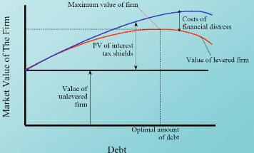
Figure 1: The optimal amount of debt to reduce the
company cost of capital Source: Principles of Corporate Finance
In the French farming industry, the NPV methodology is nearly
never used. When this method is
used, discount factors are chosen without
clear explanations, and we can observe important
variations between practitioners, even in the same business
unit. Is it because everyone considers that there is merely no risk in farming
business? However, such hypothesis does not make sense considering that a farm
manager needs to handle the weather risk, the crop's pests risk and the price
volatility risk. Is the WACC methodology not applicable in farming business, or
just the NPV method is not enough known and risks related to farming business
poorly assessed?
1.1 The Farming Business in France
French agricultural exportations represent USD 17.5 billion
(€ 13.2 billion) (Agreste, 2011; IMF.Stat, 2012), making France the
14th biggest exporter of agricultural products in 2010 (WTO, 2011).
Regarding food, France is the number three exporter in 2010, with USD 47.8
billion (€ 36.2 billion)(Agreste, 2011; WTO, 2011; IMF.Stat, 2012). France
is also the number one agricultural producer in Europe, with € 62.0
billion in 2009 over a global European production of € 327 billion
(Agreste, 2010). This high level of production and exportations is allowed by
two factors: productivity and surface. The total cultivated area (TCA) in
France represents 29.3 M ha in 2009, over the total 54.9 M ha of France
(Agreste, 2010), and wheat yields of 7.04 T/ha are 88% superior to the world
average of 3.74 T/ha (FAO, 2012).
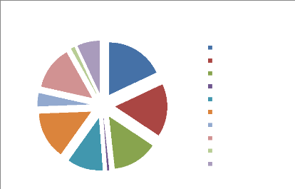
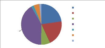
However, the high level of production in France is not due to
the size of the farms, because the average farm in France is only 55 ha in 2010
(Agreste, 2011 b) against 350 ha for US farms (Ambassade de France à
Washington, 2009). The diversity of production is really high in France as we
can see in Figure 1, as no production represent more than 16% of the overall
production in value.
Grains
Oilseeds and soyabean Sugar beet
Other plants
Fruits & vegetables Wines
Forage crops
Cattle
Poultry
Milk
Source: Insee 2011 in Billion euros
Agricultural production in France, 2010
4,1
10,1
8,8
7,3
3,6
10,5
9,4
7,8
2,8
0,8
0,4
Figure 2: Agricultural production in France,
2010
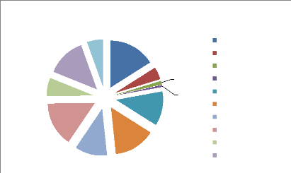
Regarding Isère, the production is also really
diversified as we can see in Figure 3. The overall production represents €
516 million for 2010, for a total GDP of around € 33 billion in
Isère for 2009 (CCI Rhône Alpes, 2011). The average size of the
farms in the department is smaller compare to France with only 38 ha in 2010
(Agreste, 2011 c), and the TCA in Isère (241 300 ha) represents only
0.8% of the national TCA.
3,0
Source: Agreste 2011 in Million euros
21,0
75,0
Agricultural production in Isère, 2010
69,0
6,0
57,0
36,0
72,0
93,0
84,0
Grains
Other plants
Fruits & vegetables Wines
Forage crops
Cattle Poultry Milk
Other animal productions Services
Figure 3: Agricultural production in Isère,
2010
1.2 The Profitability Heavily Relies on Subsidies, Not
on Investment Decision
To understand the farming business in France, it is necessary
to know the Common Agricultural Policy (CAP) and its impacts on Agriculture.
The CAP is the first and most important common policy for the European Union,
and its cost jeopardized the overall EU budget for years (Figure 4). The CAP
finds its origins in the 1950's, when European agriculture was on its knee
after World War II. Charles De Gaulle considered this policy as essential to
prevent major social events in France (Moravcsik, 1999), as he said that
agriculture was as important as the troubles in Algeria. This Policy helped to
increase the productivity, stabilized the agricultural markets, and secured
food supplies of all European countries (Clipici, 2011; Zaharia, Tudorescu,
& Zaharia, 2009; Howarth, 2000). According to Howarth (2000), its main
objectives given at its start in 1962 were:
- Agricultural productivity improvements
- Fair incomes for farmers
- Agricultural markets stability
- Secure food supplies
- Reasonable prices for customers
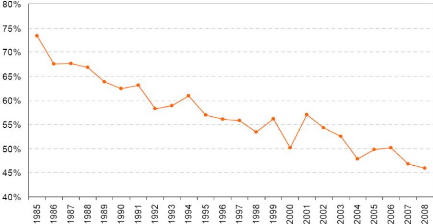
Figure 4: The percentage of the EU budget allocated to
the CAP Source: Eurostat, in Clipici 2011
However, the European CAP had been heavily criticized over its
history, either by European partners such as the Cairns group (Australia,
Brazil...) and the USA (Spencer, 2003), or by European countries also such as
the United Kingdom or Germany (Howarth, 2000; Elekes & Halmai, 2009;
Moravcsik, 1999). The major points of friction are the market distortions
induced by the CAP, the cost of this policy and the impact on the poorest
economies (Howarth, 2000; Spencer, 2003; Borrel & Hubbard, 2000; Rickard,
2001). Some authors even argued that world agricultural prices could rise by
38% if subsidies were turned off (Borrel & Hubbard, 2000). Many
negotiations rounds took place over the last decades to reduce these
distortions, and the CAP was reformed many times since 1992 (see Figure 5).
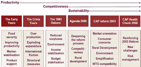
Figure 5: Historical Development of the CAP Source:
Clipici E., 2011
In 1992, the CAP was reformed to decrease export subsidies and
market supports to shift to coupled
direct payments. Those payments (direct
aids in Figure 6) were proportional to the surface cultivated
by farmers, but not directly to the volume of production. This
reform helped to reduce the production surpluses, and world agricultural
markets distortions were reduced. However, the distortions were still
significant after the reform as the overall amount of subsidies was really
high, around € 35 billion in 1992 (Clipici, 2011). All the other reforms
had the objective to reduce these distortions, such as the decoupled payments.
New conditions for granting were also added to the CAP such as environmental
protection, risk management, animal welfare, budget reduction, etc...
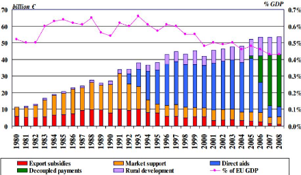
Figure 6: CAP spending evolution Source: DG
Agri
According to the Farm Accountancy Data Network (FADN), the
amount of subsidies represents 80% of the average recurring net profit for
French farms (see Table 1). Besides, grain producers depend even more on the
CAP than other types of farms.
|
2006
|
2007
|
2008
|
2009
|
2010
|
|
Subsidies
Recurring net profit before tax
Dependence on
subsidies
|
30
37
81%
|
29
46
63%
|
29
36
81%
|
29
21
138%
|
31
45
69%
|
Table 1: Subsidies and recurring net profit before tax in
France per farm, in K€ Source: FADN (RICA)
This dependence on subsidies is negative for innovation, as
all the production is oriented by the CAP and not by the market demand.
Moreover, the profitability depends on the capacity of the farmer to maximize
the subsidies. New-Zealand is an example of a country that stopped all
subsidies in 1984 (Gardner, 1994; Saunders, Wreford, & Cagatay, 2006;
Sandrey & Scobie, 1994), and enjoys nowadays an enviable situation in the
world agricultural market. This small country is the world largest milk
exporter (Evans, 2008), and the second largest sheep producer (FAO, 2012).
Another element limits the innovative capacity of French
farms, and also their adaptability: the control of the surface. As a matter of
fact the SAFERs, Societé d'Aménagement Foncier et
d'Etablissement Rural, have the power to control the land market.
According to their mission, these structures have 3 main objectives:
- Protect and revitalize agriculture: this objective means to
help young farmers to start their
activity, avoid the concentration on big farms, and develop a
peri-urban agriculture and organic farming. The major tool used here is the
preemption, which allows the SAFER to break a sale between to farmer to sell
the land to another farmer. Small and young farmers have the priority in this
system.
- Develop the vitality of the town and country planning policy:
the SAFER has the ability to
preempt some properties to help young entrepreneurs to start
their activity.
- Protect the environment: this last objective is really wide,
and goes from rehabilitation of
swamps to biodiversity protection and restructuration of the
forests...
The result of this policy is easily presented in Figure 7.
More liberal countries such as Denmark, the Netherlands or the United Kingdom
have much bigger farms, with an average capital assets per farm respectively of
1 820 000 €, 1 700 000 € and 1 370 000 €. On the contrary,
French farms have an average capital asset per farm below 400 000 €.
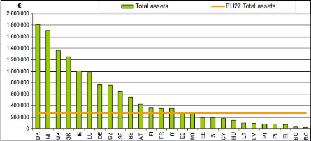
Figure 7: Average asset value per farm by member state
2007 Source: FADN
Some investments cannot be amortized in such small structures,
like methanation units for milk farms or precision farming for field crops. For
a methanation unit, which allows to reduce the impact on the environment by
producing electricity, the total investment is around 1 200 000 € for 250
kWe (AREC, 2011). This type of unit is not very important in terms of
productivity and can be 10 to 20 times bigger, but is already out of reach for
a small farm.
1.3 A New Approach to Find
The CAP has created an artificial market for French farmers.
As seen in Figure 8, the guaranteed wheat price (in blue) was well above the
world market price (in red) before 1992. The price volatility of agricultural
commodities has always existed, with a fall from 165 €/T in 1988 to 80
€/T at the end of 1990, but French farmers were protected from this high
volatility.
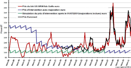
Figure 8: Volatility of the price of wheat after
application of Agenda 2000 Source: Offre et Demande Agricole
In fact, French farmers were affected by the world market
price in 1995/96, when the prices reached 180 €/T, and in 2007 when all
agricultural commodities prices soared... The price fall of 2008 and the new
peak in 2011 and 2012 illustrates well that the volatility is not coming to an
end.
Another element will modify the market for French farmers: the
end of the quotas for milk and sugar beet producers in 2015 (Pinson, 2012;
Hénin, 2011). Nowadays, the volume of production is limited for each
European milk and sugar producers, in order to avoid surpluses and price falls.
This suppression of the quotas will modify the milk and sugar market, and price
volatility will surely increase (
terrenet.fr, 2012; Hénin,
2011).
Moreover, many other countries are more competitive than
France for milk production (Rhein, 2009). The example of Germany is often cited
in France because the price of milk is lower, farms are bigger, more productive
and specialized (You, 2010; Waintrop, 2010). However, even Germany is
considered as non-competitive in the world market (Rhein, 2009). In fact, both
countries are declining in terms of market share for total agricultural
products exportation (see Figure 9). However, the case of France is more
complicated, as from the second world exporter in 1995 we lost market shares
almost continuously because of a lack of competitiveness (Momagri, 2012).
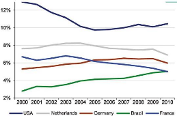
Figure 9: Fluctuation of the share of agro-food exports
by key countries in the global volume of agro-food exports
Finally, the CAP shall be reformed once more in 2014-2015: the
decoupled payments should converge at the European average and more dependant
to environmental conditions (Le Boulanger, 2011; Hénin, 2012). The
effect will be important for French producers, as the decoupled payments will
be reduced on average, particularly for grain producers. Moreover, these
payments will be conditioned to environmental obligations which are not always
respected so far.
Therefore, this is essential for farmers to analyze
the source of their actual profitability if they want to face the challenge of
a globalized agriculture combined with the reduction of subsidies! It
is necessary to evaluate each projects and farms with more accuracy
than before, because all indicators suggest that the market risk will
increase.
2 Literature Review
2.1 Risk
2.1.1 Risk in Agriculture
The risks associated with the agricultural activities can be
divided into 4 types of risks according to the OECD (Harwood, Heifner, Coble,
Perry, & Somwaru, 1999; Holzman & Jorgensen, 2001):
- Market/price risks: these risks can affect directly a farm or a
region through the variation of
the prices of land, inputs, production...
- Production risks: hail or frost can affect directly a plot, but
other climatic hazards can have a
strong impact on production. Technology evolution also can
affect the production risks, by
controlling it (dams to prevent flood, anti-hail net, drainage,
phytosanitary products...)
- Financial risks: some farmers have non agricultural
revenues. A change in these revenues may affect the profitability. Farms are
also exposed to financial risks through the interest rate on their loans.
- Institutional or legal risks: these risks are really hard to
measure, as it goes from the
responsibility risk to the legislation risk and the CAP reform
risk.
Overall, the risks in agriculture are really wide, and farmers
cannot handle them all by themselves. Production risks for example cannot be
covered only by insurance, because reinsurance companies refuse to cover the
risk of insurance companies for this type of multi-risks insurance. The
portfolio risks of these insurance is ten times higher than more conventional
sectors (Chambers, 1989; Miranda & Glauber, 1997). Therefore, policy makers
should integrate these elements into the CAP reform of 2014-2015.
On the other side, the market risks can be managed by the
farmers themselves, the futures markets can be used by farmers to reduce their
risk exposition (OECD, 2009). Actually, only 1% of all transactions made on the
futures markets are effectively physically traded, but not many farmers use
this tool (Rose, 2008). Even if the futures markets are not an efficient tool
to predict the future physical prices, they remain efficient to reduce the risk
exposure (OECD, 2009).
Regarding financial risks, it is harder to handle with
agricultural policies or tools such as the future markets. However, farmers can
with the help of their consultants estimate their financial exposition and
reduce it by choosing fixed interest rates when they subscribe new loans. It is
also possible to act on the optimal leverage level by choosing the appropriated
financing decision for new projects or equipments.
Finally, institutional or legal risks are really hard to
predict or reduce. For responsibility risk of course, it can be reduced through
insurances and the choice of equipments in accordance with the legislation.
However, institutional risks such as CAP reforms cannot be easily managed by
farmers themselves.
2.1.2 Risk Premium
The equity risk premium, also called the risk premium, represents
four different concepts according to the literature as stated by Fernandez
(2010):
- Historical equity premium (HEP): it represents the difference
between the historical results
of the stocks over government bonds or treasuries. This value
really depends on the time-frame chosen. Damodoran (2011) recommends using a
long time frame, as well as the French tax authority (2006).
- Expected equity premium (EEP): it is the expected difference
between the same elements
than the HEP. However, in this case the historical results are
not the base of the calculations. - Required equity premium (REP): this method
is used by investors to estimate the
«incremental return of a diversified portfolio (the market)
over the risk-free rate».
- Implied equity premium (IEP): it is in fact the REP assuming
the market price of the stock
represents the fair and true value of the stock.
Out of the 150 textbooks studied by Fernandez (2010), 129
authors consider that REP has to be equal to EEP. This is the most common
assumption as the CAPM states this assumption too, and 119 authors recommend
using the CAPM (Fernandez, 2010). Out of those 129, 82 consider that EEP is
also equal to HEP. We can consider that this position is the most commonly
used, as 27 authors do not explain in their textbooks how they obtained their
EEP (see Table 2). The overall recommended risk premium average is 6.7%.
However, we can see than the difference between the min and max is really wide,
ranging from 3.0% to 10.0%.
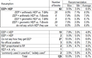
Table 2: Assumptions and recommendations of the 129 books
that assume that REP = EEP. Source: Fernandez 2010
For our calculation, we will retain from this meta-analysis
the minimum and maximum average for the most common assumption which is EEP =
HEP. Therefore, the most probable range for the risk premium would be
[5.5% : 6.7%] for the geometric mean and [7.0% : 8.5%] for the arithmetic mean.
The geometric mean is presented by many authors as less dependent of the
fluctuations and somehow more reliable. Fernandez itself recommends
3.8% to 4.3% for Europe and US.
According to the famous authors Brealey & Myers with Allen
in their editions of Principles of Corporate Finance, they recommend
to use REP between 5.0% and 8.5% (see Table 3). However, the major tendency is
to use a REP between 6.0% and 8.0%.
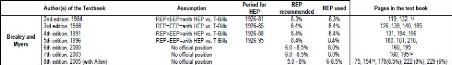
Table 3: Equity premiums recommended and used in
textbooks. Source: Fernandez 2010
What is more interesting is the reduction in the recommended
risk premium in the textbooks over the last years. Figure 10 shows that this
reduction was drastic between 1988 and 1993, and after 2002. Nowadays, the
recommendation seems to be just below 6%. It is common to see in the literature
some claims that these EEP are overvalued at 5.0 or 6.0%. Claus & Thomas
(2001) states that after 1985 it is not realistic to take long period of
centuries, and that the EEP is closer to 3.0% in reality. For France, for the
period 1985-1998, they consider that EEP should be 2.6%, basing their
calculation on the abnormal earnings approach. Quiry & Le Fur (2012) come
to a similar conclusion even with a long time frame (111 years) with a 3.2%
HEP.
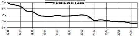
Figure 10: Moving average (last 5 years) of the REP used
or recommended in 150 finance and valuation textbooks. Source: Fernandez
2010
The French tax authority does not have a clear position on the
subject (Direction Générale des Impots, 2006), however it gives
the precision that someone could use the HEP of a long-run period: 5% over the
last 100 year in France. For the French market, Damodoran (2011) and Salomons
& Grootveld (2003) recommend to use 4.91%, using a 1976-2001 timeframe. The
Credit Suisse in its Global Investment Returns Sourcebook of 2011 (Damodoran,
2011) recommends to use 6.0% for France (for a timeframe of 1900-2010,
including the 2008 crisis for short-term Governments). Table 8 summarizes the
different HEP obtained for the French market. Most of the observations are in
the range between 3.8% and 5%.
Claus & Thomas (2001)
Direction Générale des Impôts (2006)
Damodoran (2011)
Salomons & Grootveld (2003) Quiry & Le Fur (2012)
Fernandez (2010) for European markets
1985-1998 2.6%
100 years 5.0%
1900-2010 6.0%
1976-2001 4.91%
1900-2010 3.2%
Long term 3.8% to 4.3%
Average
4.26%
Table 4: Historical Equity Premium for the French
market
The small-capitalization premium is subject to controversies
in the early literature (Damodoran, 2011), however it seems that overall we can
observe some significant premia for small or micro-capitalization. Figure 11
represents the premium observed for micro-capitalization compare to all-US
stocks. We can easily see that during the 1980's and the major part of the
1990's the small firms did not perform more than the overall US stocks.
However, since 1999 it seems that this small firm premium is starting again to
be observed.
The other element we can learn from Figure 11 is that the
variability is really strong. Therefore, it explains easily that we find really
different positions in the literature, ranging from no premium to extreme
values. For example Bergstrom, Frashure & Chisholm (1991) consider that for
the French market this premium is 8.8% for a timeframe of 1955 to 1984. For the
same time frame, they found only 3.0% for the German market.
Dimson & Marsh (2001) considers that the micro-cap
geometric premium is 5.4% over all equities for a time-frame of 1955-1999 in UK
(the EEP obtained is 6.2% for all equities for the same time frame). This
premium for the US market seems to be lower according to Leonard (2009), with a
premium ranging from 2.38% to 2.47% for US micro-cap stocks over the overall
market (time frame: 1938- 2007). This micro-cap US premium has increased after
the Dotcom crisis, reaching 5.63 to 5.83% for the period Oct-2002 to Sept-2007
(Leonard, 2009). Israelsen (2009) found 1.81% premium for small-cap compare to
mid-cap and 2.8% for small-cap compare to large-cap for a 1980-2008 time frame.
Switzer (2010) considers that this premium has even increased more when we
consider a 2001-2010 time frame reaching 7.74% in the US. For the 1926-2010
time frame, this premium is 2.03% for the US. For Canada, this small-cap
premium seems to be lower, ranging from 0.10% (1987-2010) to 4.12% (2001-2010).
The most important finding of this work is that small-stocks have better premia
during the periods of recoveries (after the dotcom crisis, the 2008 crisis, or
the 1975 crisis). This is particularly essential today, as the overall economy
is still recovering from the 2008 financial crisis.
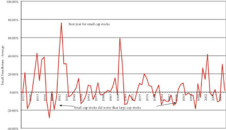
Figure 11: Small firm premium (bottom 10% of market cap
in US) between 1927-2010. Source: Damodoran 2010
Overall, the small and micro-cap premium observed ranges from
0.1% to 8.8%, depending on the market and the time frame studied. However, it
seems that this premium is increasing since 2000, because the economy has
experienced two important crisis since 2001. Moreover, it seems that the
premium seems to be higher in France from what have been observed by Bergstrom,
Franshure and Chisholm (1991). Table 5 presents a summary of our findings in
the literature.
|
Authors
|
|
Time frame
|
Small and micro-cap premium
|
|
Bergstrom, Frashure
|
&
|
1955-1984, France
|
8.8 %
|
|
Chisholm (1991)
|
|
|
|
|
Israelsen (2009)
|
|
1980-2008 US
|
1.8% to 2.8%
|
|
Leonard (2009)
|
|
2001-2007 US
|
5.63% to 5.83%
|
|
Leonard (2009)
|
|
1938-2007 US
|
2.38% to 2.47%
|
|
Switzer
|
|
2001-2010 Canada
|
4.12%
|
|
Switzer
|
|
1926-2010 Canada
|
0.10%
|
|
Switzer
|
|
2001-2010 US
|
7.74%
|
|
Switzer
|
|
1926-2010 US
|
2.03%
|
|
Mean
|
|
|
3.97%
|
Table 5: Historical Equity Premium for small and
micro-cap
For the recent time frame, which is the most appropriate time
frame considering the fact that the economy is in recovery since the major
crisis of 2008, authors considers that the HEP is ranging from 4.12% to 7.74%
(Table 5, Switzer, 2010). Moreover, this choice is supported by the fact that
many analysts agree on the fact that the soft commodities prices should
remain at a higher price in the coming years (OECD-FAO, 2010).
The expected market return should increase in the following years.
2.2 The WACC Theory
2.2.1 The Importance of the WACC Theory.
The WACC is not considered easy to compute, but is one of the
fundamental elements in modern finance (Quiry & Le Fur, 2012; Brealey,
Myers, & Allen, 2008). The NPV calculation and the determination of the
value of the stock are based on the results of the WACC, which underlines its
importance (Quiry & Le Fur, 2012, p. 699). The underlying theory of the
WACC is the CAPM. This model objective is to measures capital assets value
depending on the risk and the expected return of the company. According to
Brealey, Myers & Allen (2008), the after-tax WACC represents more the
reality of the company and can be described as follow:
E
WACC = K(D) . (1 -- Tc) r, + K(E)
K(D): cost of debt, at market value.
Tc: corporate tax rate.
D/V: total debt divided by total firm value. K(E): cost of
equity.
E/V: total equity divided by firm value.
The cost of equity in the WACC theory has to be calculated using
the CAPM, which can be described as follow:
E (Re) = Rf + f3. [E (Rm) -- Rf]
E(Re): expected return on equity. It corresponds to K(E) in the
WACC formula [3: beta. It represents the risk.
E(Rm): expected return of the market in which the company
operates. See part 2.1.2 page 20 on risk premium for the literature review
dealing with risk premium. However, the risk premium is defined as the premium
obtained compare to a risk-free asset.
Rf: risk free rate of return. The risk-free rate of return can be
estimated by the long-term government bond yield (Brealey, Myers, & Allen,
2008; Quiry & Le Fur, 2012).
2.2.2 The Betas for Micro-Capitalizations
In this research, financial techniques are used to estimate
the risk for listed companies to apply it for non-listed small companies. The
bias introduced is consequent, as the beta has a negative relationship with the
size of firms (Binder, 1992; Al-Rjoub, Varela, & Hassan, 2005; Shomir, Pat,
& Jeong-gil, 2011). Therefore, small farms should have a higher Beta
compared to listed companies operating in agriculture, as smaller firms present
little or no diversification (Drew & Veeraraghavan, 2003). Table 6 presents
the results found in the literature comparing large capitalizations and
micro-capitalizations, which can be considered as the right comparison between
the listed companies operating in agriculture which have activities in many
countries and the small farms of Isère.
|
Authors
|
Time frame
|
Number of groups
|
micro-cap Beta
premium
|
|
Al-Rjoub, Varela & Hassan (2005)
|
1970-2000
|
1st decile vs 10th d
|
|
0.51
|
|
Al-Rjoub, Varela & Hassan (2005)
|
1982-2000
|
1st decile vs 10th d
|
|
0.36
|
|
Al-Rjoub, Varela & Hassan (2005)
|
1990-2000
|
1st decile vs 10th d
|
|
0.24
|
|
Shomir, Pat & Jeong-gil (2011)
|
1980-2003
|
1st quartile vs 4th q
|
|
0.21
|
|
Bhardwaj & Brooks (1993)
|
1926-1988
|
1st group vs 5th g
|
|
0.72
|
|
Chan & Chen (1988)
|
1949-1983
|
1st group vs 20th g
|
|
0.69
|
|
Dongcheol (1993)
|
1926-1990
|
1st decile vs 10th d
|
|
0.58
|
|
Jegadeesh (1992)
|
1954-1989
|
1st group vs 20th g
|
0.32
|
- 0.62
|
|
Mean
|
|
|
|
0.47
|
Table 6: Market capitalization effect on the beta for
micro-capitalization
As presented in Table 6, the effect of size is quite important
on the beta. It is important to notice that the standard deviation also
increases with the beta (Drew & Veeraraghavan, 2003; Dongcheol, 1993; Chan
& Chen, 1988). From the results found in the literature, for
micro-capitalizations compare to large capitalizations, the beta increases on
average by 0.47, which is really significant regarding the impact of the beta
on the WACC formula.
2.3 Discount Rates and the CAPM Used in Agriculture
The CAPM and the actualization rates have already been used in
agriculture long ago. The Capital Asset Pricing Model has been tested for
example to test the farm real estate market by Barry P. J. in the 1980's (Barry
P. J., 1980a). His conclusions were that the low betas (0.19 for the US)
observed for farm real estate made this investment valuable as a
diversification tool for portfolios and that the required rate of return for
the US farmland was 8.76%. Other studies have been done on the same subject to
test the interest for investors to diversify into farmland (Hanson & Myers,
1995). It seems that these conclusions remain true nowadays, as the foreign
investments in farmland increased strongly after the rise of the grain market
price in 2007.
Since then, the diversification into agricultural commodities
have been tested either. The results are interesting, because thanks to
negative correlation with other markets, this diversification reduces the risk
and are considered as profitable for investors (Sminou, 2010). The opposite
have been tested also, to see if farmers who own their lands have an interest
to diversify their investments with traditional financial tools (Nartea &
Webster, 2008). According to their results for New Zealand after the
deregulation of the market, the expected return of the farmers would increase
thanks to diversification, even if the expected return on farmland due to
capital gains (9.83%, 1988-2003) were higher than the expected returns of
ordinary shares (5.59%, for the same period). This potential gain comes from
the good diversification of the portfolio which reduces the risk but not the
overall return according to the authors.
On the other side, some studies have been done in agriculture
using the NPV method. Most of them
do not explain clearly how they chose
their discount factors. For example, investments in peach
orchards in India
have been tested with three discount rates proposed by NGOs: 6, 9 and 12% to
compare the NPV method with the amortization method (Gangwar,
Singh, & Mandal, 2008). Finally the authors retained the 12% discount
factor.
Barry P. J., at the beginning of the 1980's, has done a
research to evaluate the impacts of government support price programs on the
financial structure of the farms of US (Barry P. J., 1980b). In his
calculation, he used three pre-tax discount factors of 10%, 12% and 14%,
corresponding to an after tax discount factor of 7.8%, 8.16% and 7.0%
respectively. However, here the author selected the three pre-tax discount
factors arbitrarily.
More recently, Johnson M. R. (Johnson, 2002) presented its
method to calculate the capitalization rate for Kansas in a case study. He
starts first with the loan rate offered to farmers, and then he adds a
discretionary increase based on the risk premium and the tax effect. He obtains
a capitalization rate of 14.71% in 2000 (with a loan rate level of 8.94% and a
corporate tax rate at 30%). Using his method we would obtain around 10.5% of
capitalization rate for France (with a loan rate level of 3.5% and a corporate
tax rate at 33%). The discount factors found in the literature are therefore
ranging from 7.0% for the lowest, to 14.71% for the most recent study found
from the US. However, it would be hard to apply these methods to the French
context, because most of these discount factors are somehow based on
discretionary risk premiums or they are chosen totally arbitrarily.
3 Research Methodology
One of the main objectives of this research is to give new
decision tools for farmers' consultants to evaluate the expected profitability
of their customers' projects or farms. In this section, the preparation of this
research will be presented.
3.1 Survey Construction
A small survey designed to collect different perspectives from
accounting and consulting companies, mainly from the network CEFRANCE:
- First, the network of the CERFRANCE represents more than 50%
of the market of farming consulting. The remaining market shares are shared by
many different organizations with no comparable size to the leader.
- Then, the methodologies used in the different CERFRANCE are
based on the same recommendations from the head of the network (the CNCER).
Therefore, we can obtain a clear view of the methodologies used by consultants
without a large survey.
3.1.1 Questionnaire
The purpose of this questionnaire is twofold:
- Confirm of reject my initial observation which stands
that farm consultants use discount rates based on loan rates plus a risk
premium around 2%.
- Test the willingness of farm consultants to use the
WACC to approximate the cost of capital of their customers in their
region.
To test these hypotheses, an internet-based survey of 9
questions was sent to 25 consultants in France. In order to improve the answer
rate, the questionnaire was sent only to farm consultants who were linked to me
in a professional social network (Viadéo® or Linked
In®). As these consultants are all French, it has been written
in French (see Appendix 3).
This choice of consultants introduces a first bias: mostly
young professionals use professional social networks. However, as young
consultants are less experimented, it is common sense to believe that they are
taught with the last methods developed or chosen by their consulting companies.
Therefore, this choice of population was motivated by its efficiency to collect
up to date information at the minimal cost.
3.1.2 Results Analysis
As the number of participants was reduced, analysis of the
results was only descriptive (percentages, average and medians) and no
statistical tests were performed. However, these results were sufficient to be
conclusive.
3.2 Historical Analysis of the Results of Farms in
Isère
3.2.1 Data Collection
The data used in this part of the research have been extracted
from the database of the CERFRANCE
Isère. This database has 5 years
of results available, for 2 000 farms operating in Isère.
CERFRANCE
Isère is the leading accounting company in the area,
serving more than 50% of the 3 999 professional
farms of the department (Agreste, 2011). Therefore, we can
consider the results extracted from this sample as representative of the
population of farmers of Isère. This is why the inclusion criteria for
the extractions were as wide as possible:
- All companies which are taxed at the
«bénéfice réel», which means that they are
obligated to produce a balance sheet, a profit and loss statement and a cash
flow statement to the tax administration. All the companies with a turnover
above 76 300 € are concerned by this obligation. This inclusion criterion
is obvious because without books accounts profitability or leverage ratios
cannot be calculated.
- All companies that are taxed under the
«Bénéfice agricole» regime, which means that more than
70% of their turnover comes from agricultural activities. This inclusion
criteria has been chosen to minimize the impact of forestry, environmental
services and other activities practiced by some farmers.
The software used at the CERFRANCE Isère (Panda) cannot
produce extractions for several years at one time neither an extraction with
all the data about a year in one file. Therefore, two extractions were made for
each year:
- One excel sheet with all the balance sheet information
available (146 data per farm, from
surface, number of labor units to asset valuation. See Appendix 1
for illustration),
- A second excel sheet with all profit & loss and cash flow
statement information (143 data per farm. See Appendix 2 for illustration)
|
Years of extraction
|
|
Number of farms after extraction Number of farms
selected
|
2006 2007 2008 2009 2010
1 060 620
1 231 620
1 199 620
919 620
1 054 620
Table 7: Primary data for the analysis of farms' results
in Isère
As presented in Table 7, the number of companies available is
not constant. This effect is due to the information system structure: depending
on the way the accounting books are send to the tax administration, the results
of the farm are automatically or manually uploaded into the database. The only
exclusion criterion was to keep a constant sample over the five years.
Therefore all farms which did not have results for 1 or more year were
excluded. This exclusion criterion reduced the population of observed farms to
620.
The 620 farms have been classified into 7 specializations,
based on the production most observed in the department of Isère (see
Figure 12). A farm generating 2/3 of its turnover from one main production was
considered as specialized in this production. Cattle ranching corresponds to
the beef production (sheep or other ruminants were considered as diversified
production as they do not represent enough farms to constitute a group). Walnut
productions, vegetables and fruit growing
were not analyzed as the number of farms observed was too low to
make groups based on their financial leverage.
256
13 28 11
45
141
Dairy farming
Grain
Cattle ranching Diversified production Vegetables
126 Walnut production
Fruit growing
Figure 12: Number of farm for each
specialization
3.2.2 Data Processing
The raw data extracted from the database were to be analyzed.
First, the self-employed labor unit costs are not always taken into accounts
into the books, due to accounting regulations. Therefore, the data have been
transformed to include a labor cost for each labor unit at the SMIC (minimum
salary level in France for a FTE, Table 8):
|
Years
|
2006
|
2007
|
2008
|
2009
|
2010
|
|
SMIC before social tax per month
|
1 254.28€
|
1 280.07€
|
1 308.88€
|
1 337.70€
|
1 343.77€
|
Table 8: Cost of each labor unit per month for the
SMIC
Another element had to be transformed in order to have
reliable results: social security contributions. This cost is tax deductible,
but depending on the legal form of the company it can be treated outside of the
balance sheet and profit & loss statements. The calculation of these
contributions depends on many factors, such as the year of installation of the
farmer, his average profits for the last 3 years (an option exists to calculate
it only with last year results). An important element is that only farmers who
operate in limited liability legal form have the possibility to treat these
contributions off-balance sheet. Their results are most of the time
significantly higher, justifying that the added contributions should be on
average higher than the contributions in books. The contributions were
calculated based on the results of the annual accounting results (in reality,
the years' results are taxed over 3 years: N-1, N-2 and N-3 for most farms).
This recalculation introduced a bias in this research, but the accounting
principles of the company have been adapted to avoid this bias for future
researches. For 2012 and after, all social contributions will be recorded in
the database.
|
Years
|
# of companies without
social security contribution in books
|
Average contribution added
|
|
Average contribution in
books
|
Average
contribution for the population
|
|
2006
|
77
|
(12%)
|
7
|
061
|
€
|
7
|
193 €
|
7
|
176 €
|
|
2007
|
110
|
(18%)
|
11
|
871
|
€
|
7
|
009 €
|
7
|
871 €
|
|
2008
|
139
|
(22%)
|
12
|
633
|
€
|
7
|
371 €
|
8
|
551 €
|
|
2009
|
153
|
(25%)
|
10
|
124
|
€
|
8
|
230€
|
8
|
697 €
|
|
2010
|
162
|
(26%)
|
6
|
539
|
€
|
7
|
488 €
|
7
|
241 €
|
Table 9: Social security contributions
3.2.3 Research Questions
The main goal of this analysis is to test the traditionalist
approach which states that an optimal level of debt helps to reduce the WACC
(Brealey, Myers, & Allen, 2008, p. 485). If this theory holds in
agriculture, a positive link between the debt level and profitability or
productivity should be observed. Therefore, the research question can be stated
with two hypotheses.
The dependant variables tested are:
- ROA: return on asset.
- ROE: return on equity.
The Independent variables tested is:
- Level of debt of the company.
First hypothesis:
H0: ROA and ROE tend to increase with the level of debt
of the farms in Isère.
H1: ROA and ROE have no positive links with the level of
debt of the farms in Isère
Second hypothesis:
H0: Financial distress may occur when leverage increases,
reducing ROA or ROE. H1: No signs of financial distress are clearly observed
when the leverage increases.
The second hypothesis is common sense. However it has to be
tested for agriculture. Milk production was really stable for years, because
the market was controlled thanks to the system of quotas. Therefore, as the
volume of production is somehow easy to control, financial performances of the
farms are easy to predict, limiting strongly the risks of financial
distress.
3.2.4 Data Analysis
The WACC theory assumes that there is an optimal debt level to
reduce the cost of capital of the company and then increase its overall
performance (see Figure 1 page 12). Therefore, ROE and ROA were analyzed by
groups of leverage in order to verify if this theory holds in agriculture. The
groups more leveraged should have better results in terms of ROE and ROA than
low leverage groups. We should also observe more variability and/or lower
results for groups with really high leverages like group 1 or 2 (Table 10).
This observation would be considered as financial distress.
As presented in part 3.2.2, the data had to be processed to be
exploited. The ROE, ROA and leverage also have to be calculated considering the
specificity of the accounting standards used at the CEFRANCE Isère.
Therefore, ROE and ROA were calculated as follow:
E
P -- w E + P c P -- w
-- P
L
- P: Profit,
- Wc: cost of labor (each FTE self-employed unit of labor
received a cost of the SMIC),
- E: shareholders equity. As no financial market exists to
estimate a market value of farm's
equity in agriculture, the book value had
to be retained,
- Pca: partners current accounts. These amounts are considered
as debt from an accounting perspective. However, it is not considered by
convention as a debt but as shareholder's equity from a consultant perspective
because these «partners» are the shareholders,
- A: total assets,
- L: leverage,
- D: total debts. The value retained was book value, as the
database do not includes
information allowing a recalculation at market value. However,
the interest rate was analyzed at the market value,
- tl: total liabilities.
|
Leverage
|
L < 20%
|
20%= L <40%
|
40%= L <60%
|
60%= L <80%
|
80% < L
|
|
Group #
|
5
|
4
|
3
|
2
|
1
|
Table 10: Groups of debt level
In order to compare the groups, a set of statistical tests
were performed with the software Statgraphic Centurion:
- Shapiro Wilk test and Kolmogorov test for the normality of
the datasets. Density trace and histograms were also used for sample sizes
bigger than 2 000 farms (Shapiro Wilk test cannot be performed for this size of
samples). Normality was tested before each test.
- One-way ANOVA and multiple range comparison to compare the
means of the different groups when the assumptions of normality and homogeneity
of variance were verified.
- When the assumption of normality or homogeneity of variance
was rejected, a non parametric test was used (Kruskal-Wallis). As normality and
equivalence of the variance are the base-assumptions of the ANOVA, the means
cannot be compared if these two hypotheses are not verified. The Kruskal-Wallis
test compares the rank of each observation to overcome this limitation, and
tests if the medians are significantly different or not.
- Mood's and Median test to analyses the medians. It is a
non-parametric test which compares the distribution of each sample around the
overall median of all the groups. Therefore, this test can estimate if the
medians are significantly different.
First, the effect of time was tested. As time has an effect on
ROE or ROA, separate tests were performed for each year in order to isolate the
time effect and analyze the effect on leverage more accurately. Then, the
effect of specialization was tested. As specialization has an effect on ROE or
ROA, separate tests were performed for each specialization to improve the
robustness of the results. The risk error (alpha) represents the risk to reject
the null hypothesis tested when it should be
considered actually true. Because 10% is an acceptable level of
risk error in finance, this alpha was used for all statistical tests in this
research.
3.3 Bond Yield Plus Risk Premium Model
The first method to estimate the capitalization rate was the
method used by the French tax authority. Farming consultants have to keep in
mind that their valuation methods can be used as the base of the calculation
for a capital gain on the sale of a company. The tax authority therefore has
the right to modify the tax base if it considers that the results do not
represent a fair value at the time of the transaction. The most common tax
adjustment in those cases is the hidden donation, when the tax authority
considers that the company or its shares (not publicly tradable in the case of
most farms) are undervalued. This is why it is necessary to include the methods
used by the administration in this study. In reality, this method is based on
the CAPM, as the risk premium is the difference with the total expected return
minus the risk-free return. The actualization rate formula can be presented in
this way:

A: Actualization rate,
Rf: Risk free rate,
â: Beta,
Rp: Risk premium for the French market.
3.3.1
Risk-Free Rate
As presented by Sharpe (1964) it was assumed that everyone can
borrow or lend its funds at a «pure rate of interest». This risk-free
rate is considered by the tax authority as the government bonds rate (Direction
Générale des Impots, 2006), and was assumed in this paper as
equivalent to the French government debt reference rate, given by the French
central bank (a 12 month average of the 10 years bonds monthly average was
used).
3.3.2 Beta and Risk premium
The risk free rate has to be increased by a risk premium,
justified by the necessary supplementary yield that a risky asset needs to
deliver compare to a pure interest rate. The tax authority recommends using the
historical risk premium observed in the French economy, which can be increased
to consider the size of the company studied. For the calculations, the
references of the tax authority were used, and an increase to consider that we
are dealing with micro-capitalization.
The first bias that arises is easy to consider, as stated by
Damodoran (2011), would be to include 2008 stock results in our time-frame: the
major crash observed this year would diminish the results significantly,
leading investors to think that the risk would be lower after the 2008 crisis
than before. However, from a pragmatic point of view, this could be considered
as logical: there is less risk of a major historical crisis after it happens
than before, like there are less risks of a centenary flood after ones
happen.
The Beta is used to consider the risk relative to the company
and the sector in which it operates (Direction Générale des
Impots, 2006). Once again, the tax authority produced some recommendation and
we will base our calculation on it. We will compare this beta with the beta
observed by another author for agriculture in France.
3.4 WACC Estimation
Regarding the WACC estimation, 2 types of data will be used:
primary and secondary data. For primary data, we will use:
- Results of the farms from Isère extracted from the
database of the CERFRANCE Isère to calculate the weighted average
leverage by specialization. The time frame of the dataset is 2006-2010, with
620 farms. The characteristics of this dataset are presented in detail in part
3.2.
- Sample collection of 46 recent loan's rate for all
specialization in the database of the
CERFRANCE Isère, to determine the market value of the cost
of debt.
Regarding secondary data, we will use:
- The market capitalization and the beta calculated by Bloomberg
for all the companies listed
in North America and Western Europe for the following
activities: Oilseed farming, grain farming, cattle ranching and farming,
poultry, fruits & vegetables. Those activities have been chosen because
they are really close to the specialization of the farms of Isère.
- Risk-free rate of return: the 10 year government bonds yield
calculated by the French central bank will be used. The 12 month average of
this rate will be used. This choice of long term maturity was determined by the
timeframe of the investments of French farms. Even in grain production,
investments are made for 7 years on average, and the rotation timeframe for the
crops is 3 to 4 years. For dairy farms, constructions are amortized over 20
years on average.
- Risk premium for small companies, as determined in part
2.1.2.
The extraction from Bloomberg helped to identify 41 companies
specialized in agriculture in Western Europe and US (see Table 11). The grain
market is globalized today, and the meat market is really influenced by world
prices either. These statements are not so true for the dairy market, because
the cost of refrigerated transportation is quite high regarding the price of
milk. The European market is a more representative market for dairy production
therefore.
The beta of each firm will be weighted averaged with the
market capitalization, in order to obtain a beta for each specialization and
each region. However, for grain farming we will retain the beta of oilseed and
grain farming for Western Europe and the US together. The grain market is so
interconnected between Europe and US that the market-risk is really close. For
the grain farming in Isère, we will retain the beta of oilseed farming
and grain farming, because oilseed production is considered as grain production
in the French classification. For dairy and cattle farming, we will retain the
beta of cattle ranching and farming of Western Europe. For diversified
production and the average farm of Isère, we will retain the average
beta of the 41 companies extracted from the Bloomberg database.
|
Specialization
|
Total market cap
(M $)
|
# of companies in western Europe
|
# of companies in
the US
|
Total # of companies
|
|
Oilseed farming
|
5 810
|
11
|
0
|
11
|
|
Grain
|
14 421
|
9
|
4
|
13
|
|
Cattle ranching
|
8 196
|
4
|
3
|
7
|
|
poultry
|
2 321
|
1
|
2
|
3
|
|
Fruits & vegetables
|
2 224
|
3
|
4
|
7
|
|
Total
|
32 971
|
28
|
13
|
41
|
Table 11: Number of companies studied for the Beta
estimation. Source: Bloomberg
The last element of the WACC formula is the corporate tax
rate. This element is really hard to determine in agriculture, because farmers
have the choice between the corporate tax rate at 15% (up to 38 120 € of
net income and 33.33% after) and the personal income tax with its progressive
tax rate from 0% to 41%, depending on the total income per capita of the
household. Moreover, the net income is also subject to social tax, at an
average rate of 32.1%. Therefore, to simplify our calculation we will assume a
corporate tax rate at 33.33%, which is the usual corporate tax rate in France
(only companies held at 75% by persons have the benefit of the 15% tax rate up
to 38 120 €). This rate is chosen in most studies about profitability for
other industries in France. Therefore, it will simplify comparisons. As the
French farms are small companies, it is not obvious that this tax rate could
increase in the coming years. The actual government considers that SEM's are
too much taxed compare to the blue chips.
4 Data Analysis
4.1 Results of the Survey
Fourteen farm consultants answered to the survey, from almost all
regions of France (Figure 13). Therefore, the results are not influenced by
only one CERFRANCE.
1 Region of the respondents
2
1
4
1
3

West North

North west East
South east South west
Center
Figure 13: Region of the CERFRANCE of the
respondents
Regarding the age and the gender, the major part of the
respondents are male consultants aged between 26 and 35 years old as we can see
in Table 12.
|
18-25 y
|
26-35 y
|
35-50 y
|
51- and more y
|
|
Age
|
1
|
11
|
2
|
-
|
|
Male
|
1
|
10
|
2
|
-
|
|
Female
|
-
|
1
|
-
|
-
|
Table 12: Age and gender of the respondents
Out of the 14 respondents, 13 said that they realized project
business plans for their customers. However, only 79% said that they used
discount factors to evaluate the value of their customers' companies in
question 5. Less surprising are the answers to question 6, where 89% answered
that they used the NPV method to estimate the profitability of a project (see
Table 13).
Do you realize project business plans for your customers?
Do you use discount factors to evaluate the value of your
customers' companies?
Do you use NPV to evaluate the profitability of your customers'
projects?
|
# of answers
|
Yes
|
No
|
NSP
|
|
14
|
13
|
1
|
-
|
|
14
|
11
|
2
|
1
|
|
9
|
8
|
1
|
-
|
Table 13: answers to question 4, 5 and 6
Regarding question 7, only 9 out of the 14 respondents
answered to the question (Table 14). It seems that the most popular method
among the farm consultants is to choose a discount factor based on the
experience, and loan's rate plus risk premium is the second most popular
method.
|
Percentage
|
# of answers
|
|
Loan's rate + risk premium
|
44%
|
4
|
|
T-bills + risk premium
|
33%
|
3
|
|
WACC
|
33%
|
3
|
|
Estimation based on experience
|
56%
|
5
|
|
Other (please specify)
|
11%
|
1
|
|
TOTAL
|
100%
|
9
|
Table 14: Answers of question 7: «how do you choose
the discount factors you use?»
Regarding the most important question of the survey, the
question 8, not all consultants are specialized in all the fields concerned by
the question. This explains why the number of answers is reduced (9 consultants
gave at least one answer for this question). However, the answers tend to
confirm that almost all farm consultants use really low discount factors (see
Table 15). The highest answer is 15% for grain producers. However, even this
answer is surprising, because this consultant uses a 5% discount factor for
cattle ranching, which seems to be a difference too important. There are merely
no reasons for such a difference in terms of risk premium between the two
different productions, and it is probable that this answer is only a typing
error.
|
# of answers
|
Mean
|
Median
|
Min
|
Max
|
|
Grain producers
|
6
|
5,5%
|
4,0%
|
1,0%
|
15,0%
|
|
Cattle ranching
|
6
|
4,0%
|
4,5%
|
1,0%
|
9,0%
|
|
Wine production
|
4
|
2,8%
|
2,5%
|
1,0%
|
6,0%
|
|
Other
|
7
|
3,3%
|
4,0%
|
1,0%
|
7,0%
|
Table 15: Answers of question8 «what discount factor
do you use usually for your customers? (ex given: 11%)»
Another element is surprising: means and medians are really
low for all production, with discount factors equivalent to the French 10 years
Government bond yield. This rate was recently at its record low at 2.422%
(Dobson, 2012). The risk premiums used by some practitioners are actually lower
than the 2% used at the CERFRANCE Isère. The low number of bankruptcy
observed in the sector (1.6%o in 2011 for Rhone Alpes) may explain that
practitioners using rates based on experience use really low risk premium. Most
of the consultants do not use a loan's rate plus 2% risk premium, as this
method would give results closer to a 5 to 6% interval (regarding the loan's
rate observed in the sector).
|
# of
answers
|
percentage
|
|
Necessary for the discernment of your recommendations
|
7
|
78%
|
|
Useful to improve the discernment of your recommendations
|
2
|
22%
|
|
Not useful regarding the efficiency of the tools you already
use
|
-
|
-
|
|
The WACC and the discount factors are not useful in your
recommendations
|
-
|
-
|
|
TOTAL
|
9
|
100%
|
Table 16: Answers of question 9: «If you were
proposed a tool to estimate the WACC of the farms of your region to use it as a
discount factor, how would you consider this tool?»
Finally, question 9 (Table 16) implicitly confirmed that
consultants are not really secured with the tools they use. 78% of the
respondents considered that a tool to estimate the WACC of the farms of their
region would be necessary to improve the discernment of their recommendation,
and the remaining 22% considered it as useful.
The major highlights of the survey are:
- Consultants use the loan rate plus risk premium model.
The risk premiums used seem to be lower than 2%,
- The most popular method it to choose estimation based
on the experience,
- Most of the consultants would find necessary to have
new tools to improve their methods.
4.2 Calculation of the Historical Results Using the
Data from CERFRANCE Isère
The objective of these calculations is to see if the
hypothesis of the traditionalist's approach is verified in agriculture: does
the performance of the firm increases with leverage? Therefore, the results of
firms divided in 5 groups of leverage were analyzed (group 1 high leverages,
group 5 lowest leverages. See section 3.2.4 page 31 for details).
4.2.1 Normality of the Datasets
Figure 14 presents the distribution of values for ROE to
compare it with a normal distribution. The distribution does not fit with the
normal distribution line looking at the histogram, because the central values
have an abnormally high frequency. This impression is confirmed by the
KolmogorovSmirnov test, because the P-Value is lower than 0.000. We can reject
with 99% confidence that ROE comes from a normal distribution. The Shapiro-Wilk
test cannot be performed because the sample is bigger than 2000 values.
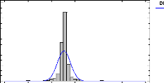
Figure 14: histogram of frequency for ROE
The distributions of ROE have been tested for each year's
separately, and within each year's for each
production either. Over the 25
tests, ROE could come from a normal distribution only for dairy
Dstrbuon
Normal
producers and cattle producers in 2010. Therefore, only the
Kruskal-Wallis and Mood's Median tests were used to analyze ROE, and the
results of the Anova's were not presented.
Figure 15 presents a histogram of the frequency of the
distribution for ROA to compare it with a normal distribution. From a graphic
perspective, it seems that ROA is closer than ROE to a normal distribution, as
the normal distribution line is closer to the frequency histogram. However, the
Kolmogorov-Smirnov test P-Value was lower than 0.000 as well, therefore we can
also reject at 99% confidence that ROA comes from a normal distribution.
-3 -1 1 3 5 7


Figure 15: Histogram of frequency for ROA
Same as the ROE, the distributions of ROA have been tested for
each year and within each year for each production separately. All the tests
performed reported the same results: ROA does not come from a normal
distribution at 99% confidence. Therefore, only the results of the
Kruskal-Wallis and Mood's Median tests were discussed for ROA.
4.2.2 ROE
4.2.2.1 ROE Tested by Time and Specialization
The dataset have been tested first to see if time had an effect
on ROE. The results of the Mood's
median and Kruskal-Wallis tests were quite
logical: as someone could have predicted, time has a
significant effect on
the ROE, with really low P-Values. The years 2006 and 2009 were two years of
isra A
bad results for farmers in Isère. The price of
agricultural commodities soared in 2007 and 2008,
explaining that these two
years were better. The effect was similar in 2010, when commodity prices
Dstributon
recovered from the severe fall of 2009. .
Mood's Median Test for ROE by YEAR Total n =
2840
Grand median = 0,0583012
|
YEAR
|
Sample Size
|
n<=
|
n>
|
Median
|
90,0% lower CL
|
90,0% upper CL
|
|
2006
|
568
|
326
|
242
|
0,0195117
|
0,00305438
|
0,041546
|
|
2007
|
568
|
245
|
323
5
|
0,0910952
55
|
0,0759334
|
0,110756
|
|
2008
|
568
|
250
|
318
|
0,0837851
|
0,065602
|
0,0957051
|
|
2009
|
568
|
328
|
240
|
0,0176906
|
0,00193535
|
0,0337506
|
|
2010
|
568
|
271
|
297
|
0,0734001
|
0,0512998
|
0,091961
|
Test statistic = 46,0986 P-Value = 2,3492E-9
Kruskal-Wallis Test for ROE by YEAR
|
YEAR
|
Sample Size
|
Average Rank
|
|
2006
|
568
|
1275,31
|
|
2007
|
568
|
1547,93
|
|
2008
|
568
|
1517,84
|
|
2009
|
568
|
1287,11
|
|
2010
|
568
|
1474,32
|
Test statistic = 57,0073 P-Value = 1,2328E-11
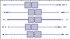
Figure 16: Box and whisker plots with median notch for
ROE by year (means are shown with a red cross)
Figure 16 presents the box and whisker plots with median notch
at 90% confidence intervals, showing that the results of the years 2006 and
2009 were significantly lower than in 2007, 2008 or 2010. Therefore, in order
to isolate the time effect, ROE has to be analyzed year by year.
ROE has been analyzed by specialization:
- Dairy production,
- Cattle ranching,
Bnd
- Grain production,
- Diversified production.
Mood's Median Test for ROE by SPECIALIZATION
Total n = 2840
Grand median = 0,0583012
|
SPECIALIZATION
|
Sample Size
|
n<=
|
n>
|
Median
|
90,0% lower CL
|
90,0% upper CL
|
|
Dairy
|
705
|
326
|
379
|
0,0747834
|
0,0595245
|
0,0896643
|
|
Cattle
|
225
|
154
|
71
|
-0,00274151
|
-0,0266764
|
0,0162487
|
|
Grains
|
630
|
299
|
331
|
0,0769898
|
0,0493805
|
0,103964
|
|
Diversified
|
1280
|
641
|
639
|
0,0580287
|
0,0458927
|
0,0699453
|
Test statistic = 36,2307 P-Value = 6,69281E-8
|
Dairy
Cattle
Grains
Diversified
|
|
Figure 17: Box and whisker plots with median notch for
ROE by specialization (means are shown with a red cross)
The Mood's median test for ROE by specialization illustrates
that the specialization has a significant impact on the ROE, with a really low
P-Value illustrating that we cannot reject the hypothesis that the medians are
different at 99% confidence. The cattle production has a median ROE lower than
the other productions. The P-Value for the Kruskal-Wallis test is 3,96451E-8,
giving the same results. Therefore, ROE was tested separately for each
specialization and each year, in order to isolate the effect of time and
specialization.
4.2.2.2 ROE for Dairy Producers
The group of dairy producers represents 141 different farms
studied over the 5 years. The Figure 18 presents the results of the Mood's
median tests performed for the ROE of the different groups. First, we can see
that the groups 4 and 5, which are the lowest leverages, have the lowest
medians. Then, the group 1 shows sign of financial distress: it has the best
results in 2007 with a ROE higher than 15%, but is close to be the worst group
in 2006 with a ROE close to 0,0%. Groups 2 and 3 seem to be more stable and
closer in terms of results, with an advantage for group 2 which is higher than
group 3 (except in 2006, a bad year for agriculture in Isère as already
presented, explaining that financial distress may have occurs for the most
leveraged farms).
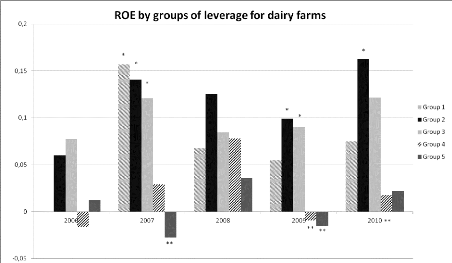
Figure 18: Median ROE for each year and each group of
leverage for dairy * means significantly higher than **
In 2007, group 1, 2 and 3 were significantly better than group
5. In 2009, it was group 2 and 3 which were significantly better than groups 4
and 5. In 2010, only the group 2 over performed the group 4. For all the other
years, there is no statistical difference between groups, and the differences
between the medians cannot be interpreted due to high standard deviation (see
Appendix 8 for details page 89).
4.2.2.3 ROE for Grain Producers
The group of grain producers represents 126 farms of
Isère. The sample is constant over the 5 years.
The Figure 19
represents the ROE for each year and each group. First, group 1 over performed
in
2006, 2009 and 2010. This is quite surprising, because 2009 wasn't a good
year in terms of price of
grains, and we could have expected signs of financial
distress. However, except in 2010, there is no statistical difference showing
that group 1 is better than any other groups. This could be surprising
regarding the major difference seen in the histograms, but standard deviations
are really high for group 1, with a lot of extreme values (see Appendix 10 page
99 for standard deviations).
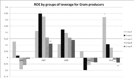
Figure 19 : Median ROE for each year and each group of
leverage for grain * means significantly higher than **
In 2007, the group 2 has significantly better results than the
group 5. For 2010, it is group 1 which has better results than groups 4 and 5.
For 2006, 2008 and 2009, no statistical conclusion can be made because the
Mood's Median and Kruskal-Wallis tests did not reveal any significant results,
with P-Values higher than 10% (see Appendix 10 page 99).
4.2.2.4 ROE for Cattle Ranching
For the group of cattle producers, only 45 specialized
producers were represented. As the sample is really small, the differences
between the groups are in most cases not significant due to the limited number
of values in each group of leverage (see Appendix 9 page 95). In figure 18
group 2 seems to over perform the other groups. Years 2007, 2008 and 2010 seem
to illustrate that performance increases with leverage, up to a limit at 80%
where financial distress may occurs. However, Group 2 is significantly higher
than group 5 only in 2008. We cannot conclude anything else from the results of
the statistical tests.
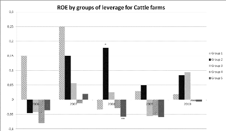
Figure 20: Median ROE for each year and each group of
leverage for cattle * means significantly higher than **
4.2.2.5 ROE for diversified production
This group is the biggest in terms of number of values, with
256 farms analyzed for 5 years. However, this is a really heterogeneous group,
with farms that cannot be compared between each others. Therefore the
diversified group was not analyzed in details because the results would not be
useful in terms of managerial implications.
4.2.2.6 Results Summary for ROE by Groups of
Leverage
Table 17 presents a summary of the results of the statistical
tests. The group 2 showed the best results in terms of ROE, followed by group
3. Groups 4 and 5 on the contrary have really often significantly lower results
than groups 2, 3 and in one case group 1.
|
Year
|
|
Dairy
|
|
|
Grain
|
Cattle
|
|
Diversified
|
|
2006 2007 2008 2009 2010
|
1
2
|
& 2
& 3
2
|
-
& 3 -
> 4
> 4
|
>
&
|
5
5
|
-
2 >
- 2 > 2 >
|
5
4
4
|
-
-
2 > 5
-
-
|
2
|
& 3
2
2
|
-
> 4 -
> 5
> 5
|
& 5
|
Table 17: Results of the Mood's median tests summary for
ROE by groups of leverage for each years
Table 18 presents the average ROE for all specializations and
all years. Diversified and dairy farming have really close results regarding
their overall means. However, it seems that diversified production is much more
volatile, moving from 13.9% ROE on average in 2007 to 4.0% in 2009. For milk,
the range starts from 5.4% in 2006 and goes to 11.7% in 2008. It seems that
this specialization is less risky than diversified production or grain farming.
Cattle's farming, on the contrary, has always the lowest results except in
2010. It seems that the economical performances of these farms are
chronically insufficient. 2010 is an exception, with the rise
of the price of meat linked with the new export opportunities to Turkey. This
improvement of the market conditions for cattle farming still has to be
confirmed, because it depends so far on a customer representing more than 50%
of the exports: if Turkey stops its importations as it did in the past, prices
could fall sharply.
|
Specialization
|
2006
|
2007
|
2008
|
2009
|
2010
|
Mean
|
|
Dairy
|
5,4%
|
9,3%
|
11,7%
|
7,8%
|
5,6%
|
8,4%
|
|
Cattle
|
-5,4%
|
3,5%
|
3,6%
|
1,5%
|
13,7%
|
2,2%
|
|
Grain
|
2,0%
|
21,2%
|
18,6%
|
2,7%
|
7,7%
|
11,3%
|
|
Diversified
|
4,0%
|
8,7%
|
13,9%
|
4,3%
|
12,3%
|
8,3%
|
|
Mean
|
3,2%
|
10,3%
|
13,0%
|
4,8%
|
10,1%
|
8,2%
|
Table 18: Weighted average ROE for all specialization and
by years
However, a really different outcome can be observed looking at
Table 19, which presents the ROE by specialization and by groups of leverage
(all years are considered in this table). The cattle specialization, which
obtains low results every year except in 2010, is profitable when the leverage
is higher than 40%. On average, the farms of Isère are economically more
profitable when the leverage increases, particularly for milk and cattle. We
can observe a fall in the results for group 1, particularly for dairy farms,
which can be explained by the financial distress that can occurs when leverage
is too high.
|
Specialization
|
Group 1
|
Group 2
|
Group 3
|
Group 4
|
Group 5
|
Mean
|
|
Dairy
|
-2,4%
|
11,7%
|
9,3%
|
6,3%
|
3,7%
|
8,4%
|
|
Cattle
|
1,2%
|
7,3%
|
7,4%
|
1,3%
|
-4,8%
|
2,2%
|
|
Grain
|
9,4%
|
12,5%
|
11,5%
|
12,0%
|
10,5%
|
11,3%
|
|
Diversified
|
5,7%
|
12,4%
|
11,1%
|
4,4%
|
5,4%
|
8,3%
|
|
Mean
|
4,6%
|
11,8%
|
10,2%
|
5,9%
|
4,8%
|
8,2%
|
Table 19: Average ROE by specialization and by
group
These results are totally consistent with the initial
hypothesis which states that there is an optimal level of debt for farming.
From the ROE results, group 2 and group 3 obtain the best results, which is an
indication that the optimal leverage lies between 40% and 80%. Group 3 has
similar results than group 2, except for dairy production. Therefore, the
optimal leverage must be higher for this specialization.
The major highlights for the analysis of the ROE are:
- Performance increases significantly with financial
leverage,
- Financial distress may occur for all production for
leverage higher than 80%.
4.2.3 ROA
4.2.3.1 ROA Tested by Time and Specialization
We applied the same tests for ROA than for ROE. The time effect
was first tested as well as
specialization to see if it was necessary to
isolate their effects on the ROA. The results were very
similar than for the
ROE, which is really logical as ROE and ROA have the same numerator. Again,
the
box and whisker plot in Figure 21 illustrates that year 2006
and 2009 were bad in terms of results for farming in Isère with ROA
median close to 1%, which is lower than the 1.5% inflation in 2006 (Le
Monde.fr, 2007).
Kruskal-Wallis Test for ROA by YEAR
|
YEAR
|
Sample Size
|
Average Rank
|
|
2006
|
568
|
1253,72
|
|
2007
|
568
|
1552,39
|
|
2008
|
568
|
1545,22
|
|
2009
|
568
|
1269,77
|
|
2010
|
568
|
1481,39
|
Test statistic = 73,6591 P-Value = 0 Mood's Median Test
for ROA by YEAR Total n = 2840
Grand median = 0,034619
|
YEAR
|
Sample Size
|
n<=
|
n>
|
Median
|
90,0% lower CL
|
90,0% upper CL
|
|
2006
|
568
|
339
|
229
|
0,00945275
|
-0,000555481
|
0,0218933
|
|
2007
|
568
|
242
|
326
|
0,0570648
|
0,0460463
|
0,0689174
|
|
2008
|
568
|
248
|
320
|
0,0528593
|
0,0436125
|
0,0621654
|
|
2009
|
568
|
327
|
241
|
0,0121847
|
0,000872383
|
0,0184358
|
|
2010
|
568
|
264
|
304
|
0,044225
|
0,0338877
|
0,0561194
|
Test statistic = 58,6901 P-Value = 5,46618E-12

B-andW hier P
Figure 21 : Box and whisker plots with median notch for
ROA by years (means are shown with a red cross)
Therefore, we had to isolate the time effect to isolate its
effect on the ROA.
Regarding the effect of specialization, once again the
P-Values were really low, illustrating that we cannot reject the hypothesis
that medians are significantly different at 99% confidence. The two tables of
the Kruskal-Wallis and Mood's median tests illustrate that cattle's ranching
presented significantly lower results than all other production in
Isère.
Kruskal-Wallis Test for ROA by SPECIALIZATION
|
SPECIALIZATION
|
Sample Size
|
Average Rank
|
|
Dairy production
|
705
|
1487,12
|
|
Cattle ranching
|
225
|
1124,15
|
|
-0i4 -0i3
-0i
Grains production
|
630
|
0i2
1494,56
|
|
Diversified production
|
RO
1280
|
1399,45
|
Test statistic = 40,0263 P-Value = 1,05194E-8
Mood's Median Test for ROA by SPECIALIZATION
Total n = 2840
Grand median = 0,034619
|
SPECIALIZATION
|
Sample Size
|
n<=
|
n>
|
Median
|
90,0% lower CL
|
90,0% upper CL
|
|
Dairy production
|
705
|
331
|
374
|
0,0427384
|
0,0344119
|
0,0510433
|
|
Cattle ranching
|
225
|
153
|
72
|
-0,00207533
|
-0,0192198
|
0,012193
|
|
Grains production
|
630
|
292
|
338
|
0,0464268
|
0,0350341
|
0,0583288
|
|
Diversified production
|
1280
|
644
|
636
|
0,0337455
|
0,0277409
|
0,0419674
|
Test statistic = 35,1914 P-Value = 1,10992E-7
Therefore, we had to isolate the effect of specialization also on
ROA. The tests were performed for each specialization and each year
separately.
4.2.3.2 ROA for Dairy Producers
The farms analyzed here are the same than the ones for the ROE
for dairy producers: 141 dairy farms of Isère. Figure 22 presents the
results of the different tests performed to compare the median ROA for dairy
farms between 2006 and 2010. The results are close to what can be observed for
the ROE: groups 2 and 3 seem to over-perform the other groups.
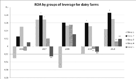
Figure 22 : ROA for each year and each group of leverage
for dairy producers * means significantly higher than **
For year 2007, the group 2 and 3 are significantly better than
the group 5. For 2009 and 2010, group
2 is significantly higher than group 4 and 5. Group 1 median on
the contrary is lower than group 2 or
3 for all years, and has the lowest median of all groups in
2006, 2008 and 2009. We cannot affirm that this difference is significant as
the standard deviations are really high for group 1 (Appendix 11 page 103).
However, these elements are clear signs of financial distress.
4.2.3.3 ROA for Grain Producers
Figure 23 represents the ROA medians for each group of
leverage for the grain producers. For this specialization, the results are not
really similar with what we can observe for the ROE. First of all, group 2 is
never statistically higher than any other groups, and is even the lowest
performance in 2008 and 2009 (without a statistical difference however). Only
2006 and 2010 tend to be consistent with the theory which states that
performance increases with leverage. In 2010 group 1 was
significantly higher than group 4. However, there was no
significant difference with group 5 even if its median was lower, because of
the higher standard deviation in group 5 (see appendix Appendix 13 page
111).
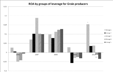
Figure 23: ROA for each year and each group of leverage
for grain producers * means significantly higher than **
The only statistical difference between groups tends to prove
that leverage increases ROA, but only one year out of five. Therefore, it will
be hard to make conclusions on these results for grain producers, except that
it seems that the optimal leverage range is 40-60% for this specialization.
4.2.3.4 ROA for Cattle Farming
The results for the ROA are consistent with what have been
observed for the ROE for cattle farming. Group 2 has a higher median than group
4 and 5 in 2008, and performance seems to increases with the leverage (see
Figure 24). Once again, group 1 do not present stable results over the year,
which could be the consequence of financial distress for those farms which are
more leveraged than 80%. However, it will be hard to make more interpretation
from these results as only 45 farms are studied for this specialization, and
significant differences are observed only in 2008.
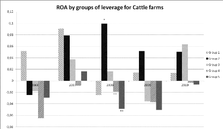
Figure 24: ROA for each year and each group of leverage
for cattle farming * means significantly higher than **
4.2.3.5 Results Summary for ROA by Groups of
Leverage
The median of group 2 is usually significantly higher than the
medians of groups 4 and 5 (Table 20). Group 3 in two cases over-performs group
4 or 5, and group 1 is better than group 4 in one case. The same elements are
observed for the ROA than for the ROE: the performance increases with the
leverage, even if the differences between groups are not always significant.
The high heterogeneity intragroup and between groups, illustrated by the high
standard deviations (see Appendix 11, Appendix 12 and Appendix 13 page 103, 107
and 111) explains why the differences cannot be considered as significant even
if it could have been anticipated so only by looking at the means and medians
of the different groups.
|
Year
|
|
Dairy
|
|
Grain
|
|
Cattle
|
|
Diversified
|
|
2006
|
|
-
|
|
|
-
|
|
-
|
|
-
|
|
|
2007
|
2
|
&3
|
>
|
5
|
-
|
|
-
|
|
3 >
|
4
|
|
2008
|
|
-
|
|
|
-
|
2
|
> 4 &
|
5
|
-
|
|
|
2009
|
2
|
> 4
|
&
|
5
|
-
|
|
-
|
|
2 >
|
5
|
|
2010
|
2
|
> 4
|
&
|
5
|
1 > 4
|
|
-
|
|
-
|
|
Table 20: results of the Mood's median tests summary for
ROA by groups of leverage for each years
Table 21 presents the average ROA for all specializations and
all years for the studied farms. The first point that can be noticed is that
the average ROA is 3.1% for the average farm in Isère. The ROA reaches
13% for grain farms in 2007, but fall to 1.7% in 2009 for the same
specialization. It is interesting to compare the dairy and the grain
production: both have a close weighted average for ROA, but variability is
really higher for grain than for dairy farming (standard deviation for dairy is
1.7%, but reaches 5.6% for Grain). Grain farming can be considered as a riskier
specialization. In 2008, the average farm in Isère reaches an ROA of
8.2%, 6.4% in 2007, and 6.2% in 2010. However,
the average cattle farm on the long term has an ROA close to the
level of inflation. 2010 is the exception with the best result of all
specialization with 9.0% ROA.
|
Specialization
|
2006
|
2007
|
2008
|
2009
|
2010
|
Mean
|
|
Dairy
|
3,3%
|
5,8%
|
7,3%
|
4,8%
|
3,4%
|
5,2%
|
|
Cattle
|
-3,6%
|
2,4%
|
2,5%
|
1,0%
|
9,0%
|
1,5%
|
|
Grain
|
1,1%
|
13,0%
|
11,9%
|
1,7%
|
5,1%
|
6,9%
|
|
Diversified
|
2,4%
|
5,3%
|
8,5%
|
2,5%
|
7,3%
|
5,0%
|
|
Mean
|
1,9%
|
6,4%
|
8,2%
|
2,9%
|
6,2%
|
3,1%
|
Table 21: Average ROA by specialization and by
years
Table 22 presents the results from a different perspective:
the high leverage groups obtain better results, except for group 1 which
presented strong signs of financial distress. The grain specialization on the
contrary have opposite results, with an ROA decreasing with the leverage.
However, when we consider this element year by year, this result cannot be
observed, showing that time has to be taken in consideration. Except for the
grain specialization, these results are consistent with what we observed for
the ROE, showing that the economical performance increases with the leverage,
and that 80% is a higher limit. Even cattle production obtains positive results
when the leverage is between 40% and 80% (group 2 and 3). In the case of this
specialization, the results of group 3 are better (without significant
difference however) than group 2.
|
Specialization
|
Group 1
|
Group 2
|
Group 3
|
Group 4
|
Group 5
|
Mean
|
|
Dairy
|
-1,1%
|
6,1%
|
5,7%
|
4,5%
|
3,3%
|
5,2%
|
|
Cattle
|
0,7%
|
4,0%
|
4,8%
|
0,9%
|
-4,2%
|
1,5%
|
|
Grain
|
3,8%
|
5,8%
|
6,8%
|
8,6%
|
9,0%
|
6,9%
|
|
Diversified
|
2,2%
|
6,6%
|
6,6%
|
3,2%
|
4,8%
|
5,0%
|
|
Global Mean
|
2,0%
|
6,2%
|
6,2%
|
4,3%
|
4,2%
|
3,1%
|
Table 22: Average ROA by specialization and by
groups
Finally, we can say that H0 cannot be rejected for the first
hypothesis and the second hypothesis tested:
- ROA and ROE tend to increase with the level of debt of
the farms in Isère.
- Financial distress may occur when leverage
increases, reducing ROA or ROE. Looking at the ROE, 80% seem
to be the upper limit. The results for the ROA tend to show that 60% is
probably more appropriate (except for dairy production).
4.3 Calculation of the Capitalization Rate Using Bond
Yields Plus Risk Premium
This method, presented in part 3.3, estimates the capitalization
or actualization rate through this equation:

A: Actualization rate Rf: Risk free rate
â: Beta
Rp: Risk premium for the French market. It has to be increased
for the micro-capitalization premium
The risk-free rate of the 10 years Governments bonds average
is 3.00% (Source French central bank, average of monthly
average from July 2011 to June 2012). It is interesting to notice that this
rate reached an average of 2.569 % in June 2012, and it has never been so low
(Dobson, 2012). The 12 month average will surely decrease in the following
months, but on the long term it cannot be considered that this rate will remain
at this low level.
Regarding the Beta, the tax authority recommends 0.8
to 1.1 for the food-processing and agricultural sector (Direction
Générale des Impots, 2006). On their side, Fama & Fench
(Laur, 2010) consider that the beta for the agricultural sector is 0.81
(time frame 1929-2009). For shorter periods of time, the agricultural
sector beta remains around 0.70 to 0.91 (Laur, 2010). In our calculation the
value of 0.8 was retained because it both answers to the
necessity to cope with the recommendation of the tax authority and the
necessity to be easy to used for consultants (these information are easy to
access).
The Risk premium is composed with two elements:
- The risk premium for the French market: from the literature
review, we found a range of [3.8% : 5.0%] (see part 2.1.2)
- The small or micro-cap premium: from the literature review, we
found a range of [4.12% : 7.74%] (see part 2.2.2).
Therefore the actualization rate has to be contained in
the following range:

The results obtained with this method are really higher than
what consultants use normally. The benefit of this fact is the
following: consultants are not exposed to tax adjustment, because the
administration cannot consider their results as hidden donation. The
administration itself would retain a lower tax base for its calculations (as
the overall price of the company is reduced by a higher actualization rate).
However, this method is only an approach based on secondary data, and need to
be compared with other approaches such as the WACC.
4.4 Approach of the WACC for Farming in Isère
4.4.1 Calculation of the Betas
Table 23 presents the results of the calculation of the betas
for the grain farming specialization. Over the 24 companies concerned, the
average beta obtained is 0.804, really close to the 0.8 to 1.1 proposed by the
tax authorities. However, it is important to notice that this beta is a
weighted average for the companies operating in grain and oilseed, with an
average market capitalization of 843 M$ (around 693 M€ for 2012). The
average total assets of the farms concerned in our study is 279 000 €.
Another element is worth noticing: the company size. The Average
grain company in Western Europe has a market capitalization of 714 M$, compared
to 1 997 M$ for North America.

|
Member Name
|
Total Mkt Cap ($)
|
adjusted beta
|
R2
|
SE beta
|
â weigthed average
|
|
SOCFIN
|
440 363 745
|
1.106
|
0.425
|
0.134
|
|
|
ODET
|
1 990 689 644
|
0.622
|
0.176
|
0.093
|
|
|
SIPEF NV
|
550 707 800
|
0.729
|
0.152
|
0.139
|
|
|
SOCFINASIA
|
598 033 371
|
0.419
|
0.010
|
0.126
|
|
|
ANGLO-EAST PLNTS
|
395 519 023
|
0.574
|
0.056
|
0.147
|
|
|
SOCFINAF
|
383 174 522
|
0.626
|
0.100
|
0.131
|
|
|
REA HOLDINGS
|
224 078 524
|
0.641
|
0.054
|
0.191
|
|
|
ADECOAGRO SA
|
834 190 505
|
1.220
|
0.246
|
0.289
|
|
|
M P EVANS GROUP
|
331 529 995
|
0.517
|
0.048
|
0.123
|
|
|
CONTINENTAL FARM
|
47 960 000
|
0.289
|
0.003
|
0.173
|
|
|
NARBOROUGH PLTNS
|
14 030 701
|
0.352
|
0.000
|
0.137
|
|
|
5 810 277 829
|
|
|
0.144*
|
0,722
|
|
ADECOAGRO SA
|
834 190 505
|
1.220
|
0.246
|
0.289
|
|
|
TRIGON AGRI A/S
|
106 214 029
|
0.870
|
0.175
|
0.174
|
|
|
BLACK EARTH-SDR
|
129 321 577
|
1.017
|
0.217
|
0.194
|
|
|
SOCFINASIA
|
598 033 371
|
0.419
|
0.010
|
0.126
|
|
|
SOCFIN
|
440 363 745
|
0.499
|
0.020
|
0.182
|
|
|
BONIFICA FERR
|
190 783 713
|
0.574
|
0.010
|
0.353
|
|
|
CONTINENTAL FARM
|
47 960 000
|
0.289
|
0.003
|
0.173
|
|
|
AGRICOLE DE CRAU
|
29 847 642
|
-0.166
|
0.008
|
1.226
|
|
|
BOLLORE
|
4 053 210 291
|
0.785
|
0.344
|
0.093
|
|
|
6 429 924 873
|
|
|
0.145*
|
0,780
|
|
ANDERSONS INC
|
663 031 853
|
1.132
|
0.377
|
0.153
|
|
|
VITERRA INC
|
4 573 354 378
|
0.834
|
0.142
|
0.184
|
|
|
SANDERSON FARMS
|
928 292 250
|
0.501
|
0.023
|
0.162
|
|
|
SEABOARD CORP
|
1 826 143 352
|
1.106
|
0.425
|
0.134
|
|
|
7 990 821 833
|
|
|
0.167*
|
0.882
|
|
20 231 024 535
|
|
|
0.154*
|
0.804
|
industry
oilseed farming in w europe
oilseed farming in w europe
oilseed farming in w europe
oilseed farming in w europe
oilseed farming in w europe
oilseed farming in w europe
oilseed farming in w europe
oilseed farming in w europe
oilseed farming in w europe
oilseed farming in w europe
oilseed farming in w europe
Total oilseed farming in WE
grain western europe
grain western europe
grain western europe
grain western europe
grain western europe
grain western europe
grain western europe
grain western europe
grain western europe
Total grain western europe
grain north america
grain north america
grain north america
grain north america
Total grain north america
TOTAL grain & Oilseed
Table 23: Calculation of the Beta for the grain
specialization (oilseed is considered as grain farming in France). Source:
Bloomberg
*weighted average of the SE for each company
For the cattle ranching, presented in Table 24, we see that
there is more difference between Europe and North America. The average beta is
really higher for the four European companies, with a beta close to 1. Once
more, the range of references proposed by the Tax authorities corresponds to
what is observed in Bloomberg. It is worth noticing the difference of the size
of the companies between the two continents, but in the opposite direction with
the grain specialization. European companies are more important, with an
average market capitalization of 319 M$ compared with an average of 68 M$ for
North America. However, the market capitalization of the listed companies
operating in cattle ranching and farming is smaller than the companies
operating in grain.
|
Member Name
|
Total Mkt Cap ($)
|
adjusted beta
|
R2
|
SE beta
|
â weigthed average
|
|
YASHENG GROUP
|
71 968 101
|
0.517
|
0.007
|
0.331
|
|
|
ALICO INC
|
133 115 937
|
0.929
|
0.259
|
0.150
|
|
|
CANAL CAPITAL CO
|
39 135
|
-2.083
|
0.018
|
3.955
|
|
|
205 123 173
|
|
|
0.214*
|
0.784
|
|
NATIONAL MILK
|
3 871 194
|
0.274
|
0.011
|
0.085
|
|
|
ADECOAGRO SA
|
834 190 504
|
1.222
|
0.246
|
0.289
|
|
|
TRIGON AGRI A/S
|
106 214 028
|
0.870
|
0.175
|
0.174
|
|
|
M P EVANS GROUP
|
331 529 994
|
0.517
|
0.048
|
0.123
|
|
|
1 275 805 720
|
|
|
0.236*
|
1.007
|
|
1 480 928 893
|
|
|
0.233*
|
0.976
|
industry
cattle ranching and farming NA
cattle ranching and farming
NA
cattle ranching and farming NA
Total cattle ranching and farming NA
cattle ranching and farming WE cattle ranching and farming WE
cattle ranching and farming WE cattle ranching and farming WE
Total cattle ranching and farming WE
TOTAL cattle ranching
Table 24: Calculation of the beta for the cattle ranching
and farming specialization. Source: Bloomberg
*weighted average of the SE of each companies
Table 25 presents the companies specialized in poultry and
fruits and vegetables. These
specializations are not studied in this paper,
because the number of farms concerned is lower in
Isère. However, some regions are more concerned with these
types of farms, and some consultants will find useful to work on these beta.
|
Member Name
|
Total Mkt Cap ($)
|
adjusted beta
|
R2
|
SE beta
|
â weigthed average
|
|
CAL-MAINE FOODS
|
|
715 100 119
|
0.814
|
0.238
|
0.128
|
|
|
SANDERSON FARMS
|
|
928 292 250
|
0.501
|
0.023
|
0.162
|
|
|
1
|
643 392 369
|
|
|
0.147*
|
0.637
|
|
LDC
|
|
677 446 072
|
0.512
|
0.083
|
0.088
|
|
|
|
677 446 072
|
|
|
0.088*
|
0.512
|
|
DOLE FOOD CO INC
|
|
633 782 418
|
1.081
|
0.254
|
0.191
|
|
|
VILLAGE FARMS IN
|
|
27 137 995
|
0.479
|
0.014
|
0.182
|
|
|
FRESH DEL MONTE
|
1
|
106 613 718
|
0.881
|
0.401
|
0.100
|
|
|
ALICO INC
|
|
133 115 937
|
0.929
|
0.259
|
0.150
|
|
|
1
|
900 650 068
|
|
|
0.135*
|
0.945
|
|
CAMPOSOL HOLDING
|
|
84 172 880
|
0.558
|
0.043
|
0.159
|
|
|
CONTINENTAL FARM
|
|
47 960 000
|
0.289
|
0.003
|
0.173
|
|
|
BONIFICA FERR
|
|
190 783 713
|
0.574
|
0.010
|
0.353
|
|
|
|
322 916 593
|
|
|
0.276*
|
0.528
|
industry
poultry north america
poultry north america
Total poultry north america
poultry western europe
Total poultry western europe
fruits&vegetables NA fruits&vegetables NA
fruits&vegetables NA fruits&vegetables NA
Total fruits&vegetables NA
fruits&vegetables WE
fruits&vegetables
WE
fruits&vegetables WE
Total fruits&vegetables WE
Table 25: Calculation of the beta for poultry and fruits
& vegetables Source: Bloomberg
* weighted average of the SE of each company
Table 26 presents a summary of the beta for the companies
specialized in agriculture for each specialization. It is interesting to notice
that the average market capitalization of North American companies is bigger
than the Western European ones, but their beta is higher. This element is not
consistent with what can be found in the literature about the relationship
between the market size of a company and its beta. Therefore, we can conclude
that the risk must be lower for farming in Western Europe than in North
America.
|
industry
|
|
|
# of companies Average Mkt
Cap ($)
|
SE beta* â weigthed
average
|
TOTAL grain & Oilseed western Europe and North
America
TOTAL cattle ranching western Europe and North
America
TOTAL Western Europe
Total oilseed farming in WE Total grain western europe Total
grain north america
Total poultry North America
Total poultry Western Europe
Total fruits&vegetables North America Total
fruits&vegetables Western Europe
|
11
9
4
24
3
4
7
2
1
4
3
28
|
1
|
528 714 997 842
68 318 211
821 677 475 107
518
|
207 436 705 959
374
951
561
696 446 162 638
441
|
075 097 458 356
391
430
270
185 072 517 864
825
|
0.144 0.145 0.167 0.154
0.214
0.236
0.169
0.147 0.088 0.135 0.276
0.153
|
Total cattle ranching and farming NA
Total cattle
ranching and farming WE
0.722
0.780
0.882
0.804
0.784
1.007
0.976
0.637
0.512
0.945
0.528
0.758

13 903 075 957 0.160 0.856
41 804 179 869 0.156 0.802
TOTAL North America
TOTAL North America + Western Europe
Table 26: Summary of the beta for the different
specialization and regions Source: Bloomberg
* weighted average of the SE of each company
4.4.2 Calculation of the WACC for the Different
Specialization
Table 27 presents the results of the different leverage for
each specialization. This leverage was be
used in the calculation of the
estimation of the WACC for each specialization. Other financial
information
are presented in this table, such as the net salary per capita (in
€/month) which can be
compared to the SMIC which is around 1 029 € net per month
for the time period 2006-2010. Therefore, the average cattle farmers in
Isère earn less than the minimum salary in France.
The average leverage is really similar for each
specialization, around 50%, but the debt coverage on the contrary is different
depending on the specialization. The grain farmers have a debt coverage of
3.16, which is really different than the 2.08 for the cattle farmers. It shows
again that cattle farming was the less profitable specialization in
Isère for 2006-2010.
|
Specialization
|
Leverage
|
Net salary per capita
|
EBITDA/turnover
|
Debt coverage*
|
|
Dairy
|
52.7%
|
1 230 €
|
41%
|
2.44
|
|
Cattle farming
|
49.5%
|
1 015 €
|
42%
|
2.08
|
|
Grain
|
49.9%
|
1 478 €
|
46%
|
3.16
|
|
Diversified
|
54.6%
|
1 277 €
|
35%
|
2.49
|
|
Weighted average
|
52.8%
|
1 279 €
|
39%
|
2.54
|
Table 27: Characteristic of each specialization in
Isère *EBITDA/total annuity
Regarding the WACC, Table 28 presents the details of the
calculation and the range of WACC for each specialization. First, the cost of
debt is really low for farmers in France (see Appendix 14 page 115).
The first element which could explain this fact is that loans are
guaranteed by the assets in the farming business, reducing therefore the risk
for the bank and the interest rate as well. The other element which
can explain this fact is that the first bank in agriculture is the
Crédit Agricole, which is really linked with the agricultural sector.
His regional boards are mostly composed with farmers.
One could object that this low cost of debt doesn't reflect
the real risk associated with the debt in Agriculture because of the
specificity of this sector. However, the rate bankruptcy is really low: 1.6%o
in Rhone Alpes (Coface, 2011). This element is linked with the culture of the
French farmers. Going bankrupt is clearly not conceivable for most of them, and
we can put this statement in relation with their level of salary. As
presented in table 27, cattle farmers on average earn less than the minimum
salary in France, but they maintain their activity and continue to pay their
annuities. From an economical perspective, this attitude is totally
counter-productive, because selling the farm and getting whatever job would
generates higher returns. This fact illustrates the farmers' attachment
to their farm and may explain the really good interest rates they obtain from
their banks.
|
Specialization
|
rE. E/V (low)
|
rE. E/V (high)
|
rD.(1-Tc).D/V
|
WACC (low an high range)
|
|
Dairy
|
7,0%
|
10,3%
|
1,3%
|
8,3%
|
11,7%
|
|
Cattle
|
7,4%
|
11,0%
|
1,2%
|
8,6%
|
12,2%
|
|
Grain
|
6,6%
|
9,6%
|
1,2%
|
7,7%
|
10,8%
|
|
Diversified
|
5,9%
|
8,7%
|
1,3%
|
7,2%
|
10,0%
|
|
Mean
|
6,2%
|
9,1%
|
1,3%
|
7,4%
|
10,3%
|
Table 28: WACC estimation for each specialization
(leverage is based on table 27)
The cost of equity is higher for dairy and cattle farms (see
Table 28), linked with the higher beta observed for these specializations.
Finally, the WACC range for the average farm in Isère is [7.4% ; 10.3%].
This method gives lower results than the method proposed by the tax
authorities. However, for some specializations, the range is almost similar,
particularly for cattle and dairy production.
Another element has to be considered. As a matter of fact, the
WACC methodology takes into
account the leverage, which reduces the overall
cost of capital. Table 29 presents the WACC for the
farms of the group 5, for which the leverage range is 0-20%. Here
the WACC increases tremendously, reaching almost 20% for the higher estimation
for cattle and dairy production.
|
Specialization
|
rE. E/V (low)
|
rE. E/V (high)
|
rD.(1-Tc).D/V
|
WACC (low and high range)
|
|
Dairy
|
13,2%
|
19,6%
|
0,3%
|
13,5%
|
19,9%
|
|
Cattle
|
13,2%
|
19,6%
|
0,2%
|
13,5%
|
19,9%
|
|
Grain
|
11,8%
|
17,3%
|
0,2%
|
12,0%
|
17,5%
|
|
Diversified
|
11,8%
|
17,3%
|
0,2%
|
12,0%
|
17,5%
|
|
Mean
|
11,8%
|
17,3%
|
0,2%
|
12,0%
|
17,5%
|
Table 29 : WACC estimation for each specialization for
group 5 (0 to 20% leverage)
Group 2 (60-80% leverage) was usually the best group in terms
of results (see parts 4.2.2 and 4.2.3). Regarding this group, the WACC falls to
lower levels, between 5.6% and 7.4% for the average farm in Isère. This
massive reduction of the WACC is due to the really low cost of debt observed in
agriculture in France. The level is still higher for cattle and dairy farms of
course, pushed by the higher beta for this production. The WACC for this group
of leverage is closer to the actualization rate used by practitioners
(2.5-4.5%), but still significantly higher.
|
Specialization
|
rE. E/V (low)
|
rE. E/V (high)
|
rD.(1-Tc).D/V
|
WACC (low and high range)
|
|
Dairy
|
4,4%
|
6,5%
|
1,8%
|
6,2%
|
8,3%
|
|
Cattle
|
4,4%
|
6,5%
|
1,7%
|
6,1%
|
8,2%
|
|
Grain
|
3,9%
|
5,8%
|
1,6%
|
5,5%
|
7,4%
|
|
Diversified
|
3,9%
|
5,8%
|
1,7%
|
5,6%
|
7,4%
|
|
Mean
|
3,9%
|
5,8%
|
1,7%
|
5,6%
|
7,4%
|
Table 30: WACC estimation for each specialization for
group 2 (60 to 80% leverage)
As presented in the previous sections, the signs of financial
distress are strong in group 1 (leverage higher than 80%), and even for the
group 2. Therefore, the real optimal WACC is maybe closer to the
results presented in Table 28 for leverages around 50%. Farming
consultants should use these ranges of WACC to determine their actualization
rates in their feasibility studies.
5 Discussion
5.1 Survey Results
The results of the survey confirmed my initial observations:
farm consultants do not often use the WACC method, and the discount factors
used are really low generally, around 2.5% to 4.5%. Moreover, the estimations
based on experience are the most popular, and we can make the assumption that
they are influenced by the low level of bankruptcy in the sector. The means of
the discount factors used by practitioners was compared to the ROE and ROA
statistically observed in Isère and the required risk premium based on
our calculation. As practitioners use lower discount factors than the required
risk premium, it signifies that the estimations they produce are overestimated,
which would lead farmers to base their decisions on overoptimistic
simulations.
5.2 ROE and ROA Analysis the Farms of Isère
The statistical tests performed in part 4 confirm the
underlying hypothesis of the WACC methodology: firm's performance increases
with leverage up to a certain limit where financial distress occurs. The
standard deviation increases in group 1, with lower median results. It can be
safely assumed that 80% leverage is a limit that should not be exceeded in
agriculture.
Groups 2 and 3 are the groups which have results significantly
better than the lower groups, meaning that the optimal level of debt could be
between 40% and 80%. As group 3 shows good results either, better than group 1
which shows strong signs of financial distress some years, it is common sense
to think that the optimal debt level is closer to 60% than 80%. Except for the
dairy specialization, it could be recommended to target a leverage of 40 to
60%.
For grain and cattle producers, the optimal level of debt is
surely between 40% and 60%. The median ROA of the group 2 is never
significantly higher than any other groups, and is even lower some years
(without significant differences). The group 3 on the contrary presents more
stable results in terms of ROA for these specializations (grain vs cattle).
This element may be explained by the difference in nature between these two
productions: dairy farms have to invest in expensive buildings and equipments,
necessary to increase the volume of production (the size of the animal housing
is directly linked with the level of production); However, for grain
production, the most expensive equipments are the tractors, and there is no
such linear relationship between the investment and the productivity. Land is
more linked with the productivity, but availability of land is not linked with
the financial capacity of farmers, and most of the time farmers rent the land.
Therefore, lands are most of the time not financed by loans and have no impact
on the leverage. For cattle farming, the animal housing is less necessary than
for dairy farms, depending on the surface of pasture available for the herd.
Therefore, a high leverage for these farms does not directly guarantee that the
farm will benefit of a higher potential of production.
Other elements can be learned from the results of the analysis
of the ROE and ROA of farms in Isère. The average farm in Isère
has not so low results in terms of ROE and ROA: 8.2% and 3.1% respectively. ROE
and ROA reaches respectively 11.8% and 6.2% for group 2, which is higher than
what consultants use. If we consider that the historical ROA should be the
minimum actualization rate, the difference with the actualization rate used by
practitioners is quite high.
On average, the respondents answered that they used discount
factors around 2.5% to 4.5% depending on the specialization. Moreover, the
results obtained in this analysis are based on historical results: it does not
take all the risks into account and reflects only the past results of the farms
of Isère. Therefore, most agricultural consultants use overoptimistic
discount factors, leading them to consider that some projects are profitable
when not.
5.3 Capitalization Using the Bond Yield Plus Risk
Premium
The range obtained using this method is [9.3% ; 12.7%], far
from the 2.5% to 4.5% commonly used by the practitioners in agriculture, and
even the historical ROA around 4.0% to 6.8% observed for the groups 2 and 3 of
the farms from Isère (leverage between 40 and 80%). On the contrary,
some specializations reached this range in terms of ROE, with 11.3% for grain.
The first conclusion we can draw from these results is that farmers of
Isère do not reach the required rate of return calculated for some
specializations. The second conclusion is that we can now safely assume that
most practitioners do not use the appropriate actualization rate in their
consulting activities, leading farmers to base their decisions on
overoptimistic results.
It is common sense to think that the first observation comes
partially from the second. As a matter of fact, most of the farmers from the
database studied in this research based their financial decision partially on
the business plans calculated by the CERFRANCE Isère. Now, it is
established that the risk premium was not enough taken into account in these
business plans, leading some farmers to start a project without an appropriate
economical assessment. This statement is particularly true when farms are sold
to new farmers, because the valuation methods used by practitioners tend to
overestimate the value of the company. In this case, the new farmer buys a farm
which is too expensive regarding its expected performances, which decreases
strongly the net present value of his investment. Eventually, this leads the
overall sector to underperform on the long run.
This eventuality is hard to prove, but has to be considered.
In Isère, the consultants calculate the price of farm using two
valuation methods, as recommended by the tax authorities (Direction
Générale des Impots, 2006). The most commonly used are the
patrimonial method and the profitability method. The first one is easy to
implement and requires the evaluation of the net assets of the farm. Buildings
and equipments are valued at their resale price. In one sense, this is the
value of the company if it had to be sold parts by parts. The second one is
based on the actualization rate: we divide the reproducible net cash flow
generated by the actualization rate. It is the NPV of a perpetual cash flow. A
difference between 3% and 9% multiplies the value of the farm by 3 with this
method! The most usual discount factors used by practitioners are 2 to 4 times
lower than the range [9.3% ; 12.7%] obtained with the method recommended by the
tax authorities, which means that the difference can be really important.
5.4 The WACC Methodology
The elements observed in part 5.3, regarding the results of
the method bond yield plus risk premium proposed by the tax authorities, are
consistent but higher than what is obtained with the WACC methodology for the
average farm in Isère. This method confirms that the actualization rates
used by practitioners are undervalued. However, it gives really different
results depending on the leverage of the companies. Therefore, it gives a
strong advantage to this approach for the practitioner, who will be able to
adapt his actualization rate to the particularity of each farm. Another
advantage is the possibility to choose the best financing solution for a new
investment, considering the overall
leverage of the farm in order to modify its capital structure to
reduce the WACC. The consequence of this modification should be the increase of
the profit generated by the farm.
On the other side, the method proposed by the tax authorities
has the strong advantage to be easier to implement and to learn for the
consultants. The other advantage of the bond yield plus risk premium as
presented by the French tax authority is its origin itself: in case of
litigation with the administration, the choice of the actualization rate will
be easier to defend with the method they recommend. The power of this argument
is reduced by the recognition of legitimacy of other methods from the
administration itself, without describing or citing them however (Direction
Générale des Impots, 2006).
Finally, we can observe that the WACC methodology should be
more accepted by the practitioners, as it gives lower results for the average
farms in Isère. This element has to be considered, because such a strong
modification of the actualization rates used by the consultants would signify
that all their previous studies were significantly wrong. It could lead to a
movement of rejection from these practitioners.
6 Utilization of These Results
6.1 Managerial Implications
The first conclusion that can be learned from this research is
that agricultural consultants do not use adapted discount factors. The lack of
research and publication on the subject is leading consultants to adopt
discount factors based on the cost of debt or inflation or even only on
risk-free assets, and not on the cost of capital or a real risk premium. The
first managerial implication that should be drawn is the necessity of further
research on the topic. CERFRANCE developed a partnership with a network of
engineering school in agriculture to specialize 40 students in consulting for
farmers every year (CNCER, 2012). This partnership with teaching and research
facilities could be the base of the discussion about the necessity to improve
the knowledge on the topic. The engineering schools in agriculture are the
perfect support for a deeper research on the subject, and this option should be
considered as the partnership with the CERFRANCE would help the researchers to
access a unique database that contains all economical results of more than 50%
of all French farmers. Finally, the CNCER (the central element of the CERFRANCE
network) should initiate a project to uniform the practices among the different
members of the network. It is clearly a weakness of the network so far.
The other implication induced by this research is the
necessity to improve the methods actually used by most practitioners of the
CERFFRANCE. Our survey is not exhaustive, therefore it cannot be said that all
the CERFRANCE are concerned, neither all its consultants. Some answers prove
that some of them use higher rates. However, generally speaking it is obvious
that the different methods to determine appropriate actualization rate are not
well understood by most of the consultants. In-house training should be more
focused on these methods, as well as on the consequences of choosing extremely
low discount factors. This type of training could start without waiting for
other results, because even the descriptive statistics show that for some
groups of leverage the average ROE and ROA are really higher than the discount
factors used by practitioners. The ROE cannot be the right estimation for a
discount factor. However, it seems to be misleading to choose it two times
lower than the ROA for the best groups of farms.
Consultants and farmers should also adapt their methodologies
for the management of the working capital. This element is really important in
agriculture, and represents 34.5% of the total assets in dairy farming in
Isère and 43% for the cattle farms. This working capital is principally
composed by the animals (66% for dairy, and 79% for cattle farms). This working
capital, for the farms that are not enough leveraged, could be financed with
debt instead of being financed with equities, which is usually the case in
agriculture. This financing is possible to put in place, as the financial
institutions could take a guarantee on the herd of cattle. The farmers would be
able to recuperate in cash a part of its equities, as well as reducing its
overall cost of capital. The benefit could be important, both for the financial
institution which would increase its activities, and also for the farmers who
would be able to increase the NPV of their farms and their personal wealth. An
estimation of the possible gain for the farmer is presented in Table 31. The
hypotheses of this calculation are:
- 4% interest rate, higher than the average rate for farms from
Isère, because the loan would be riskier for the bank than a loan
guaranteed by lands or constructions,
- 40 000 € total loan, (45% of the total value of the
animals for an average dairy farm), - 10% actualization rate,
- 6 years maturity, considering that a herd is renewed at 25%
each year on average and calves become productive in their third year.
Year
net cash flow (total)
Present Value at 10%
Positive cash flow
annual payment (4% interest) tax relief on interests (at 33%)
discount rate
NPV
|
0
|
|
1
|
|
2
|
|
3
|
|
4
|
|
5
|
|
6
|
|
40
|
000
|
|
|
|
|
|
|
|
|
|
|
|
|
|
|
-7
|
510
|
-7
|
510
|
-7
|
510
|
-7
|
510
|
-7
|
510
|
-7
|
510
|
|
|
|
429
|
|
356
|
|
281
|
|
203
|
|
122
|
|
44
|
|
40
|
000
|
-7
|
080
|
-7
|
153
|
-7
|
229
|
-7
|
307
|
-7
|
388
|
-7
|
466
|
|
1,000
|
0,909
|
0,826
|
0,751
|
0,683
|
0,621
|
0,564
|
|
40 000
|
-6 437
|
-5 912
|
-5 431
|
-4 991
|
-4 587
|
-4 214
|
|
8 429 €
|
|
|
|
|
|
|
Table 31: NPV of a refinancing operation to reduce the
WACC and increase the wealth of a dairy farm
The example presented in table 31 would not be interesting if
the actualization rate was set at 3% like most consultants do. However, it
becomes really interesting when the actualization rate is set in a normal range
for dairy farms (between 8.3% and 11.7% as presented in section 4).
The only limitation of this strategy is to get the acceptation
of the financial institution which would increase its risk exposure. So far,
the risk associated with the working capital was mostly supported by the farmer
itself. However, this limitation could be reduced if the farmers subscribe to a
predefined percentage of the cash generated by the new loan on a financial
product offered by the institution. This solution would also be interesting for
the preparation of the retirement of the farmers, who are most of the time not
well prepared considering the low level of the pensions in the sector.
6.2 Agricultural Policies Implications
The actual Common Agricultural Policy (CAP) does not take into
consideration many elements of the risk in agriculture:
- The climate risk (some subsidies are now conditioned to the
subscription to climatic
insurance, but this is a marginal phenomena yet),
- The variability of the soft commodities price.
Our results show that some years are profitable, when we
consider 2007, 2008 or even 2010. However, 2006 and 2009 were really poor in
terms of results. The future CAP will be reformed in 2014 or 2015, depending on
the complexity of the negotiations to reach a consensus among European
countries. It could be a great opportunity to consider the evolution of the
risk in agriculture during this reform. Some analysts suggest that
countercyclical tools could help farmers to maintain their revenue during
downturns and limit the overall cost of the CAP (Momagri, 2012b). This paper
shows that cyclicality of revenues and profitability are really strong.
Instability comes from the price inelasticity regarding the soft commodities: 1
or 2% change in the level of global production can lead to a price variation of
50 to 100%, and even more (Momagri, 2012b). Therefore, the opportunity of
changing the CAP to integrate countercyclical tools should be strongly
considered, even if this would lead to add complexity to a system already
considered as opaque and complex by non-initiated observers.
Other policies should be included in the CAP, which are the
public subsidies for new farmers. So far, only the French government subsidizes
the new farmers through loans at low interest rates and a front subsidy for the
first year of activity. These elements could be generalized at the European
level, particularly for the loan subsidy which could be an easy way to redirect
the CAP payments to more socially acceptable subsidies. Lower interest rates
and public support for loan's access can be as profitable in the long term for
farming activities as decoupled payments or direct aids which represent a large
part of the cost of the CAP (see Figure 6, page 16).This type of support would
have a lower impact on the price of the grains than direct payments, as it
would be more oriented on maintaining the number of young farmers high enough
to maintain the age pyramid of this population.
7 Limitations and Further Research Implications
7.1 Survey Construction
The purpose of this survey is not to have an exhaustive view
of the tools used by the practitioners in the field. As the questionnaire was
sent to consultants of different CERFRANCE, the answers cannot be considered as
representative for all accounting companies working with farmers. However, the
CERFRANCE has a dominant position in this particular market all over the
country and serve more than 50% of the farmers. Therefore, it could be
appropriate for the CNCER to intensify its researches on the subject to uniform
the practices across all CERFRANCE.
7.2 ROE and ROA Analysis
As we can see in Table 7 page 29, some years like 2009 count
fewer companies available for analysis, even if the number of books accounts
produced by the CERFRANCE Isère increased constantly over the 5 years.
Therefore, some companies were not included in the research because of
limitations of the information system. However, this limitation cannot be
considered as enough relevant to invalidate the results obtained, mainly
because the non-inclusion in the database for a company occurs randomly (there
is no reason not to include results in the database).
Another limitation comes from the decision to work on a
constant population. This constant population enables an interpretation of the
results over several years, but it also removes the companies that went
bankrupt during the studied period. Therefore, this exclusion criterion may
have an effect on the results for the hypothesis 2 which analyses the effect of
financial distress. However, the number of bankruptcy in agriculture is really
low: only 63 farms went bankrupt in 2011 in Rhone Alpes (Coface, 2011) over 39
020 farms (Agreste, 2011), which represents 1.6%o bankruptcy in the sector for
the year.
Another limitation comes from the number of farms available
for the cattle specialization. These farms, specialized in beef production are
not enough represented in Isère to obtain reliable results. Other
regions such as Côtes d'Or or Saône-et-Loire should work on the
subject.
Finally repeated measure statistical test could have been
performed to test the data to try to evaluate more precisely the ideal debt
leverage ratio. However, these mixed models are not available with traditional
statistical software as they do no compare means or medians but probabilities
(here probability to fall in financial distress in year N+1 depending on the
debt level of year N). As this research paper tries to serve as a base for all
the consultants of the CERFRANCE network, this analysis needs to be replicable
with the results of other departments without expensive tools such as SAS or
SPSS. However, this limitation justifies further researches on the topic.
7.3 Bond Yield Plus risk Premium Model
The bond yield plus risk premium model is easier to calculate
than the WACC for the farms, which represents a strong advantage for this
method. However, this model does not take into account the financial structure
of the companies studied. This strong limitation reduces its applicability to
the farms of Isère, which are really diversified.
The research was based on elements found in the literature for
this part of the research. It has been
decided to choose this method in
order to try to estimate what actualization rate could be chosen
without exhaustive researches on the subject. The purpose of
this choice is to compare the actualization rate used by practitioners with the
rates the tax authorities could use in case of litigation.
7.4 The WACC Methodology
The first limitation of this methodology is really easy to
identify: this method, based on the CAPM, is really dependent on the beta of
the company studied. However, the beta cannot be calculated for non listed
companies, and it is necessary to extrapolate the results of listed companies
to obtain an appropriate beta for the small and medium farming businesses
studied in this paper. The other limitation of the method is directly linked to
the first one: the market value of the firm should be estimated by its market
capitalization. However, for non-listed companies this value cannot be
calculated. The book value used in our research cannot replace fully the market
capitalization, because it does not reflect the opinion of the market on the
company.
The second limitation of this method is the size of the farms
studied compare to the size of the listed companies used to calculate the
betas. Even if a premium was added to the betas of the listed companies, it
remains a bias not considered by the WACC methodology.
The last limitation is more linked with the choice of the
expected return. It has been chosen on purpose to adopt the risk premium to
estimate E(Rm) - Rf, in order to be able to compare the results of the two
methodologies. However, it could have chosen to use the historical results of
the farms from Isère of the first quartile (the 25% most performing
farms).
7.5 Further Research Implications
First, there is a clear necessity to intensify the research
about the optimal level of debt in Agriculture. Repeated measure statistical
tests could be used to work deeper on the subject, in order to identify more
clearly the optimal level of debt, but also to identify what are the other
factors that have a strong impact on the financial performance of farms. It
seems obvious that the productivity of farmers (number of hectares or cows per
FTE) and the surface of the farm play a great role in the results. However, it
is really hard to find quantitative research on the subject in France, at least
researches that could be used easily by financial consultants.
The other further research implication is the necessity to
test the methods presented here in the long run, in order to compare them. It
would be interesting to follow many projects evaluated with the NPV method in
order to see finally which method gave the most appropriate actualization rate.
Moreover, other methods should be tested either to identify which ones should
be chosen by practitioners. So far, this research tends to prove that the WACC
methodology can be used by consultants, even if some theoretical limitations
arose.
Finally, the same research methodology should be applied in
other departments than Isère, with other specializations also. This
would give further indications on the adaptability of the WACC methodology to
the agricultural sector. It would allow also consultants to estimate the
appropriate discount factors for farms specialized in fruits, wines or
vegetables.
Conclusion
The WACC methodology tested in this research presents real
limitations due to its underlying theories based on the market efficiency. This
assumption holds only for the listed companies, introducing a bias in the
calculation presented in this paper. However, the results obtained are
consistent with the initial expectations regarding the relationship between
leverage and financial performance or financial distress. Therefore,
consultants should take more consideration for this methodology and use it in
their feasibility studies.
The other achievement of this paper concerns the discount
rates actually used by practitioners. All signs clearly indicate that many of
them use abnormally low actualization rates, ranging from 2.5 to 4.5%. The
impact of these low actualization rates in valuation methods, such as the
profitability method, can be really important. The NPV of a farm can be
over-estimated by two to four using such discount factors! Some consultants use
more appropriate rates, but it is far from being a generality according to the
results of the survey.
Then, it appears clearly that leverage has a positive impact
on the financial performance of the farms of Isère. These expected
results confirm that the WACC methodology should hold in the context of small
and medium farming business. Therefore, consultants should consider the capital
structure of the farms into consideration not only to avoid the risk of
financial distress, but also to look for the optimal leverage, which appears to
range between 40 and 60%. From the results presented in this paper, the 60-80%
leverage group presented really good performances, but also more variability.
Moreover, the bankruptcy risk was not studied because a sample of farms studied
had to be constant. Therefore, it is safer to consider that the optimal debt
level lies in the group 40-60%, may be closer to 60% regarding the good
performance of the 60-80% group, particularly for the dairy specialization.
Finally, the consultants of the CERFRANCE Isère do not
need to wait for other researches on the field to modify their methods. Main
recommendation is to increase significantly their actualization rates. On the
other side, it must be acknowledge that further researches on the topic are
necessary to improve the methodology and determine more precisely the
hypothesis that should be taken, regarding the risk premiums and the beta for
example. The productivity constraints of the consultants working in the
different CERFRANCE militate in favor of a partnership with the engineering
schools specialized in agriculture. This partnership, already implemented in
some schools, could be the starting point of others researches about the
financial performances of farming businesses.
Bibliography
Agreste. (2011 b). Agreste Primeur, France
Métropolitaine, Recensement agricole 2010. Montreuil Sous Bois:
Agreste.
Agreste. (2011). Commerce extérieur agroalimentaire.
Agreste Conjoncture , 2 (12), pp. 1-5.
Agreste. (2010). Memento de la statistique agricole.
Retrieved 03 23, 2012, from
www.agreste.agriculture.gouv.fr:
http://www.agreste.agriculture.gouv.fr/reperes/memento-de-lastatistique-agricole/
Agreste. (2011, September). Mémento de la statistique
agricole. Retrieved May 28, 2012, from
www.agreste.agriculture.gouv.fr:
http://www.agreste.agriculture.gouv.fr/IMG/pdf_R8212C01.pdf
Agreste. (2011 c). Premiers résultats en Isère.
Agreste Rhône Alpes, Coup d'Oeil , 129, 4 p.
Al-Rjoub, S., Varela, O., & Hassan, M. (2005). The size
effect reversal in the USA. Applied Financial Economics , 15 (17),
1189-1197.
Ambassade de France à Washington. (2009). Les Etats
Unis en chiffre. Washington DC: République Française.
AREC. (2011). la méthanisation en Poitou-Charentes
- Enjeux et perspectives. Retrieved March 29, 2012, from
www.arecpc.com:
www.arecpc.com/f245_la_methanisation_en_poitou_charentes_enjeux_et_perspectives.html
Barry, P. J. (1980a). Capital Asset Pricing and Farm Real Estate.
American Agricultural Economics Association , 62 (3), 549.
Barry, P. J. (1981). Capital Asset Pricing and Farm Real Estate:
Reply. American Agricultural Economics Association , 63 (3), 580.
Barry, P. J. (1980b). Financial Impacts of Government Support
Price Programs: Comment. American Journal Of Agricultural Economics ,
62 (3), 599-604.
Bergstrom, G., Frashure, R., & Chisholm, J. (1991).
The Gains from international small-company in Global Portfolios:
Quantiative Strategies for Maximum Performance. Homewood: R.Z. Aliber and
B.R. Bruce, Business One Irwin.
Bhardwaj, R. K., & Brooks, L. D. (1993). DUAL BETAS FROM BULL
AND BEAR MARKETS: REVERSAL OF THE SIZE EFFECT. Journal of Financial
Research , 16 (4), 269-284.
Binder, J. J. (1992). BETA, FIRM SIZE, AND CONCENTRATION.
Economic Inquiry , 30 (3), 556-563.
Birner, R., Davis, K., Pender, J., Nkonya, E.,
Anandajayasekeram, P., & Ekboir, J. (2009). From best practice to best lit:
a framework for designing and anlyzing pluralistic agricultural advisory
services worldwide. Journal of Agricultural Education and Extension ,
15, 341-355.
Borrel, B., & Hubbard, L. (2000). Global Economic Effects of
the EU Common Agricultural Policy. Economic Affaris , 20 (2),
18-26.
Brealey, R. A., Myers, S. C., & Allen, F. (2008).
Principles of corporate finance (Ninth international edition ed.). New
York: McGraw Hill.
Breisinger, C., Ecker, O., & Al-Riffai, P. (2011). Economie
du Printemps Arabe. De la révolution à la transformation et la
sécurité alimentaire. Politiques alimentaires en perspective
, 18, 2-4.
Carter, C. (1981). Capital Asset Pricing and Farm Real Estate:
Comment. American Agricultural Economics Association , 63 (3), 578.
CCI Rhône Alpes. (2011). Les Chiffres Clés de
l'Isère, édition 2010-2011. Grenoble: Chambre de Commerce et
d'Industrie de Grenoble.
Chambers, R. G. (1989). Insurability and Moral Hazard in
Agricultural Insurance Markets. American Journal of Agricultural Economics
, 85 (2), 604-616.
Chan, K., & Chen, N.-F. (1988). An Unconditional
Asset-Pricing Test and the Role of Firm Size as an Instrumental Variable for
Risk. Journal of Finance , 43 (2), 309-325.
Claus, J., & Thomas, J. (2001). ). Equity Premia as Low as
Three Percent? Evidence from Analysts' Earnings Forecasts for Domestic and
International Stock Markets. Journal of Finance , 56 (5), 1629-
1666.
Clipici, E. (2011). Directions of Common Agricultural Policy.
Agricultural Management , 13 (1), 173- 178.
CNCER. (2012, February). CERFRANCE, conseil et expertise
comptable. Retrieved June 30, 2012, from
www.reseau-cerfrance.fr:
http://www.reseau-cerfrance.fr/emploi-formation/?p=jeunes-diplomes
Coface. (2011). Observatoire des défaillances.
Retrieved May 28, 2012, from
www.coface.fr:
http://www.coface.fr/CofacePortal/ShowBinary/BEA%20Repository/FR_fr_FR/documents/observato
ire/observatoire-des-defaillances.pdf
Damgé, M. (2012, July 20). Sécheresse aux
Etats-Unis, les cours des céréales flambent. Retrieved July
21, 2012, from
www.lemonde.fr:
http://www.lemonde.fr/economie/article/2012/07/20/secheresseaux-etats-unis-les-cours-des-cereales-flambent_1736460_3234.html?xtmc=cereales&xtcr=1
Damodoran, A. (2011, February 23). Equity Risk Premiums
(ERP): Determinants, Estimation and Implication? Retrieved June 23, 2012,
from Social Science Research Network:
http://papers.ssrn.com/sol3/papers.cfm?abstract_id=1769064
Dimson, E., & Marsh, P. (2001). U.K. Financial Market
Returns, 1955-2000. Journal of Business , 74 (1), 1-31.
Direction Générale des Impots. (2006, November).
fiche descriptive 4166. Retrieved June 20, 2012,
from
www.impots.gouv.fr:
http://www.impots.gouv.fr/portal/deploiement/p1/fichedescriptive_4166/fichedescriptive_4166.pdf
Dobson, P. (2012, May 25). French 10-Year Government yield
drops to to record low 2,422. Retrieved June 03, 2012, from
www.bloomberg.com:
http://www.bloomberg.com/news/2012-05-25/french10-year-government-bond-yield-drops-to-record-low-2-422-.html
Dongcheol, K. (1993). The Extent of Nonstationarity of Beta.
Review of Quantitative Finance & Accounting , 3 (2), 241-254.
Drew, M. E., & Veeraraghavan, M. (2003). Beta, Firm Size,
Book-to-Market Equity and Stock Returns. Journal of the Asia Pacific
Economy , 8 (3), 354-380.
Elekes, A., & Halmai, P. (2009). The "Hottest Topic" of the
budgetary review: Will the CAP survive? Intereconomics , 44 (5),
300-308.
Evans, G. (2008, August 4). N.Z. Forecasts. Retrieved
March 29, 2012, from
www.bloomberg.com:
http://www.bloomberg.com/apps/news?pid=newsarchive&sid=a4O5KrquIb90
FAO. (2012, February 23). FAOSTAT. Retrieved March 23,
2012, from
faostat.fao.org:
http://faostat.fao.org/site/567/DesktopDefault.aspx?PageID=567#ancor
FAO. (2012). Major food and agricultural commodities
producers. Retrieved March 29, 2012, from
www.fao.org:
http://www.fao.org/es/ess/top/commodity.html?item=1012&lang=en&year=2005
Faure, G., & Compagnone, C. (2011). Les Transformations du
conseil face à une nouvelle agriculture. Cahiers de l'Agriculture ,
20 (5), 321-326.
Faure, G., Desjeux, V., & Gasselin, P. (2011). Revue
Bibliographique sur les recherches menées dans le monde sur le conseil
en agriculture. Cahiers de l'Agriculture , 20 (5), 327-342.
Fernandez, P. (2010, November 16). Retrieved June 30, 2012, from
Social Science Research Network:
http://papers.ssrn.com/sol3/papers.cfm?abstract_id=1473225
Gangwar, L., Singh, D., & Mandal, G. (2008). Economic
Evaluation of Peach Cultivation in North Indian Plains. Agricultural
Economics Research Review , 21 (1), 123-129.
Gardner, B. L. (1994). Liberalization in New-Zealand agriculture:
Discussion. American Journal of Agricultural Economics , 76 (5),
1053.
Hanson, S. D., & Myers, R. J. (1995). Testing for a
time-varying risk premium in the returns to U.S. farmland. Journal of
Empirical Finance , 2 (3), 265-276.
Harwood, J., Heifner, R., Coble, K., Perry, J., & Somwaru, A.
(1999). Managing Risk in Farming: Concepts Research and Analysis.
Agricultural Economic Report , 774.
Hénin, F. (2011, August 30). Fin des quotas
laitiers - PAC 2015 - Projet européen des JA -
Elevagenet.fr. Retrieved
March 31, 2012, from
www.web-agri.fr:
http://www.web-agri.fr/actualite-agricole/politique-syndicalisme/article/le-projet-europeen-de-ja-pour-installer-et-maintenir-du-lait-sur-tout-le-territoire-1145-73874.html
Hénin, F. (2011, December 10). Impact de la fin des
quotas sur les accords de prêts aux éleveurs. Retrieved April
01, 2012, from
www.web-agri.fr:
http://www.web-agri.fr/actualite-
agricole/economie-social/article/les-banques-apprennent-a-travailler-avec-la-fin-des-quotas-1142-
76501.html
Hénin, F. (2012, March 26). Réforme de la
PAC - DPU - Verdissements. Retrieved March 27, 2012, from
www.terrenet.fr:
http://www.terre-net.fr/actualite-agricole/politique-syndicalisme/article/le-nouveau-calcul-des-paiements-directs-portera-sur-55-de-l-enveloppe-des-soutiens-publics-affectes-205-79048.html
Holzman, & Jorgensen. (2001). Social Risk management: A New
conceptual framework for social protection, and beyond. International Tax
and public Finance , 8, 529-556.
Howarth, R. (2000). The CAP: History and attempts at reform.
Economic Affairs , 20 (2), 4.
IMF.Stat. (2012, 03 23). Principal Global Indicators.
Consulté le 03 23, 2012, sur
www.principalglobalindicators.org:
http://www.principalglobalindicators.org/default.aspx
Israelsen, C. (2009). The Value Premium. Financial Planning ,
39 (6), 108-110.
Jegadeesh, N. (1992). Does Market Risk Really Explain the Size
Effect? Journal Of Financial & Quantitative Analysis , 27 (3),
337-351.
Johnson, M. R. (2002). Kansas's Agricultural Use Value Method.
Assessment Journal , 9 (3), 23-29.
Laur, P. (2010). Le Beta varie-t-il pour de bonnes raisons
? L'influence des caractéristiques spécifiques des firmes et du
contexte macroéconomique sur le coefficient de risque
systématique ß. Retrieved July 10, 2012, from
www.vernimmen.net:
http://www.vernimmen.net/ftp/Memoire_Pierre_Laur.pdf
Le Boulanger, A. (2011, November 29). La PAC 2014 au coeur
des crises. Retrieved January 15, 2012, from
www.cerfrance.fr:
http://www.cerfrance.fr/blog-agri/2011/11/29/la-pac-2014-au-coeur-descrises/
Le Monde.fr. (2007, February 27). L'inflation
française est restée mesurée en 2006. Retrieved June
20, 2012, from
www.lemonde.fr:
http://www.lemonde.fr/economie/article/2007/01/12/l-inflationfrancaise-est-restee-mesuree-en-2006_854975_3234.html
Leonard, S. (2009). U.S. Equity Returns After Major Market
Crashes. Journal of Financial Planning , 22 (10), 84-94.
Miranda, M., & Glauber, J. (1997). Systemic Risk,
Reinsurance, and Failure of Crop Insurance Markets. American Journal of
Agricultural Economics , 79, 206-215.
Momagri. (2012b, June 26). Another CAP is possible.
Retrieved July 21, 2012, from
www.momagri.org:
http://www.momagri.org/PDF/momagri-GB-autre-PAC-est-possible-26-06-12.pdf
Momagri. (2012, February 27). France is gradually losing its
place among major agricultural export powerhouses. Retrieved April 02,
2012, from
www.momagri.org:
http://www.momagri.org/UK/agriculture-s-key-figures/France-is-gradually-losing-its-place-amongmajor-agricultural-export-powerhouses-_1058.html
Moravcsik, A. (1999). Le grain et la grandeur : les origines
économiques de la politique européenne du général
de Gaulle (1ère partie). Revue Française de Science Politique
, 49 (4-5), 507-544.
Mundler, P., Labarthe, P., & Laurent, C. (2006). Les
disparités d'accès au conseil: le cas de la région
Rhône-Alpes. Economie Rurale (291), 26-34.
Nartea, G., & Webster, P. (2008). Should farmers invest in
financial assets as a risk management strategy? Some evidence from New Zealand.
Australian Journal Of Agricultural & Resource Economics ,
52 (2), 183-202.
OECD. (2009). Managing Risk in Agriculture: a Holistic
Approach. Paris: Editions OCDE.
OECD. (2011). Risk management in agriculture. Retrieved
November 10, 2011, from
www.oecd.org:
www.oecd.org/agriculture/policies/risk
OECD-FAO. (2010). Agricultural Outlook 2010-2019.
Marston Gate: OECD.
Petit, M. (2006). L'exploitation agricole familiale:
leçons actuelles de débats anciens. Cahiers Agricultures ,
15 (6), 486-490.
Pinson, V. (2012, March 22). Fin des quotas laitiers:
quels enjeux pour les abattoirs? Retrieved April 01, 2012, from
www.lequotidienlesmarches.fr:
http://www.lequotidienlesmarches.fr/marches/findes-quotas-laitiers-quel-enjeu-pour-les-abattoirs-art329564-39.html
Quiry, P., & Le Fur, Y. (2012). Finance d'Entreprise.
Pierre Vernimmen 10ème édition. Paris: Dalloz.
Rhein, E. (2009, September 11). The UE needs a competitive
dairy production. Retrieved March 31, 2012, from
rhein.blogactiv.eu:
http://rhein.blogactiv.eu/2009/09/11/the-eu-needs-a-competitivedairy-industry/
Rickard, S. (2001). Time to scrap the CAP? Accountancy ,
128 (1298), 83.
Rose, F. (2008). A note on the role of investment capital in
the US agricultural futures markets and the possible effect on cash prices.
Groupe sur les céréales, les aliments du bétail et le
sucre. OECD.
Salomons, R., & Grootveld, H. (2003). The equity risk
premium: Emerging vs Developed Markets. Emerging Markets Review , 4,
121-144.
Sandrey, R. A., & Scobie, G. M. (1994). Changing
international competitiveness and trade: Recent experience in New Zealand
agriculture. American Journal Of Agricultural Economics , 76 (5),
1041.
Saunders, C., Wreford, A., & Cagatay, S. (2006). Trade
Liberalisation and greenhouse gas emissions: the case of the dayring in the
European Union and New-Zealand. Australian Journal of Agricultural &
Resources Economics , 50 (4), 538-555.
Sharpe, W. F. (1964). Capital asset prices: a theory of market
equilibrium under conditions of risk. Journal of Finance , 19 (3),
425-442.
Shomir, S., Pat, O., & Jeong-gil, C. (2011). FURTHER
INVESTIGATION ON THE VARIABILITY OF INDIVIDUAL STOCK BETA AND PORTFOLIO SIZE.
International Journal Of Business, Accounting, & Finance , 5 (1),
91-102.
Sminou, K. (2010). Stock Market and Agricultural Futures
Diversification: An International Perspective. Journal Of Alternative
Investments , 12 (4), 36-57.
Spencer, D. (2003). An agreement to deal. Economist ,
368 (8337), 65.
Switzer, L. (2010). The behaviour of small cap vs. large cap
stocks in recessions and recoveries: Empirical evidence for the United States
and Canada. The North American Journal of Economics and Finance , 21
(3), 332-346.
terrenet.fr. (2012, January 31).
mobilisation de la filière betterave contre la fin des quotas de
production. Retrieved March 31, 2012, from
www.terrenet.fr:
http://www.terre-
net.fr/cours_marches_agricoles/article/la-filiere-betterave-se-mobilise-contre-la-reforme-europeenne-du-marche-du-sucre-1395-77463.html
Waintrop, M. (2010, August 18). Pourquoi le lait Allemand
est-il moins cher que le Français. Retrieved March 15, 2012, from
www.la-croix.com:
http://www.la-croix.com/Actualite/S-
informer/Economie/Pourquoi-le-lait-allemand-est-moins-cher-que-le-francais-_NG_-2010-08-18-
555741
WTO. (2011). International Trade Statistics 2011.
Geneva: World Trade Organization.
You, G. (2010, August 17). Institut de l'Elevage: une
filière lait "low-cost". Retrieved March 20, 2012, from
www.web-agri.fr:
http://www.web-agri.fr/actualite-agricole/economie-social/article/lait-prixtroisieme-trimestre-filiere-allemande-low-cost-1142-64110.html
Zaharia, I., Tudorescu, N., & Zaharia, C. (2009). Have the
Cap Reforms Delivered Significant Changes. Economics, Management &
Financial Markets , 4 (2), 107-110.
|
Appendices
Appendix 1: Illustration of the database extraction.
File name: "extraction 2006_1"
|
|
|
70
|
|
Appendix 2: Illustration of the database extraction,
balance sheet information. File name: "extraction 2006_2"
|
|
|
71
|
Appendix 3: Questionnaire
L'objectif de cette enquête est d'avoir un aperçu
des techniques utilisées par les conseillers d'entreprise agricole pour
actualiser les flux. Les résultats de cette enquête seront
analysés de manière anonyme, et seront utilisés dans le
mémoire « L'utilisation du CMPC en vue d'optimiser
l'évaluation du coût du capital dans les exploitations agricoles
en France. Constatations empiriques à partir des résultats
économiques d'exploitations Iséroises ». Une version
électronique de ce mémoire pourra être distribuée
aux personnes intéressées d'ici octobre.

Nom de votre compagnie: Age: Sexe:
Question 1: Quelle est votre profession ?
Question 2: Pouvez-vous décrire succinctement votre
activité ?
Question 3: Dans le cadre de votre profession, rédigez
vous des études prévisionnelles pour vos adhérents afin
d'estimer la rentabilité de leurs projets ?

Question 4: est-ce que vous utilisez des taux d'actualisation
pour évaluer la valeur d'une entreprise agricole ? (actualiser un flux
perpétuel: flux prévisionnel reproductible / taux
d'actualisation)

Question 5: Est-ce que vous utilisez la méthode de la
Valeur Actuelle Nette (VAN) pour estimer la rentabilité d'un projet ?
(projet photovoltaïque ou méthanisation par exemple)

Question 6: comment choisissez vous un taux d'actualisation ?
Cochez les méthodes utilisées dans votre structure.

Question 7: Dans quelle fourchette de pourcentage se situent les
taux d'actualisation que vous utilisez principalement pour votre
clientèle agricole ?
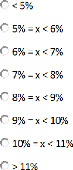
Question 8: Comment qualifieriez vous les méthodes
utilisées dans votre structure pour comparer et évaluer des
projets d'investissement ?

Question 9: Si l'on vient a vous proposer un outil pour
estimer le coût moyen pondéré du capital des exploitations
de votre région afin de l'utiliser comme taux d'actualisation, comment
considéreriez vous cet outil ?

P-Value
Appendix 4: Normality test of the datasets for ROE,
extraction from statgraphics
Uncensored Data - ROE
Data variable: ROEc
The Shapiro Wilk test for normality cannot be performed.
Therefore we observed the data graphically, and considered that the data follow
a normal distribution (density trace and histogram of frequency look
normal).
2800 values ranging from -4,78806 to 4,81454 Fitted
Distributions
Normal
mean = 0,0444249
standard deviation = 0,628166
The StatAdvisor
This analysis shows the results of fitting a normal
distribution to the data on ROEc. The estimated parameters of the fitted
distribution are shown above. You can test whether the normal distribution fits
the data adequately by selecting Goodness-ofFit Tests from the list of Tabular
Options. You can also assess visually how well the normal distribution fits by
selecting Frequency Histogram from the list of Graphical Options. Other options
within the procedure allow you to compute and display tail areas and critical
values for the distribution. To select a different distribution, press the
alternate mouse button and select Analysis Options.
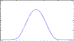
Tests for Normality for ROEc
Den
Test
Statistic
Too much data
The StatAdvisor
This pane shows the results of several tests run to determine
whether ROEc can be adequately modeled by a normal
03
distribution. The Shapiro-Wilk test is based upon comparing the
quantiles of the fitted normal distribution to the quantiles of the data. The
Shapiro-Wilk test was not performed because the sample size was greater than
2000.
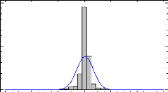
Goodness-of-Fit Tests for ROEc
Kolmogorov-Smirnov Test
|
Normal
|
|
DPLUS
|
0,187571
|
|
DMINUS
|
0,203456
|
|
DN
|
0,203456
|
|
P-Value
|
0,0
|
The StatAdvisor
This pane shows the results of tests run to determine whether
ROEc can be adequately modeled by a normal distribution. Since the smallest
P-value amongst the tests performed is less than 0,05, we can reject the idea
that ROEc comes from a normal distribution with 95% confidence.
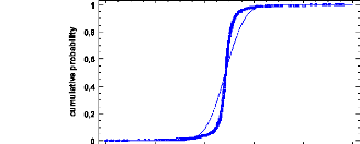
ce for RO
P-Value
Appendix 5: Normality tests of the datasets for ROA,
extraction from statgraphics Uncensored Data - ROA by time
Data variable: ROA
Too much data for the Shapiro test. We do it visually, and we can
conclude that it is normally distributed! 3046 values ranging from -4,37674 to
3,08145
Fitted Distributions
Normal
mean = 0,0569658
standard deviation = 0,485766
The StatAdvisor
This analysis shows the results of fitting a normal
distribution to the data on ROA. The estimated parameters of the fitted
distribution are shown above. You can test whether the normal distribution fits
the data adequately by selecting Goodness-ofFit Tests from the list of Tabular
Options. You can also assess visually how well the normal distribution fits by
selecting Frequency Histogram from the list of Graphical Options. Other options
within the procedure allow you to compute and display tail areas and critical
values for the distribution. To select a different distribution, press the
alternate mouse button and select Analysis Options.
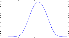
Tests for Normality for ROA
Test
Shapiro-Wilk W
Statistic D
Too much data
The StatAdvisor
This pane shows the results of several tests run to determine
whether ROA can be adequately modeled by a normal
distribution. The
Shapiro-Wilk test is based upon comparing the quantiles of the fitted normal
distribution to the quantiles of
0,3
the data. The Shapiro-Wilk test was not performed because the
sample size was greater than 2000.
|
G
K
xn
|
oodness-of-Fit Tests for ROA olmogorov-Smirnov
Test
,
|
|
Normal
|
|
DPLUS
|
0,148105
|
|
0,1
DMINUS
|
0,170935
|
|
DN
|
0,170935
|
|
P-Value
0
|
0,0
|
The StatAdvisor
This pane shows the results of tests run to determine whether ROA
can be adequately modeled by a normal distribution.
Since the smallest P-value amongst the tests performed is less
than 0,05, we can reject the idea that ROA comes from a normal distribution
with 95% confidence.
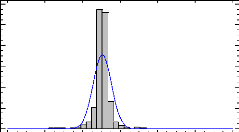
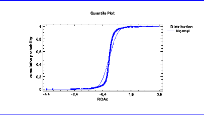
Appendix 6: ROE by year
One-Way ANOVA - ROE by ANNEE
Dependent variable: ROE Factor: ANNEE
Number of observations: 2840 Number of levels: 5
The StatAdvisor
This procedure performs a one-way analysis of variance for ROE.
It constructs various tests and graphs to compare the mean values of ROE for
the 5 different levels of ANNEE. The F-test in the ANOVA table will test
whether there are any significant differences amongst the means. If there are,
the Multiple Range Tests will tell you which means are significantly different
from which others. If you are worried about the presence of outliers, choose
the Kruskal-Wallis Test which compares medians instead of means. The various
plots will help you judge the practical significance of the results, as well as
allow you to look for possible violations of the assumptions underlying the
analysis of variance.
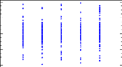
Summary Statistics for ROE
|
ANNEE
|
Count
|
Average
|
Standard deviation
|
Coeff. of variation
|
Minimum
|
Maximum
|
Range
|
Stnd. skewness
|
|
2006
|
568
|
-0,0079864
|
0,541224
|
-6776,82%
|
-3,25
|
3,7011
|
6,9511
|
1,84708
|
|
2007
|
568
|
0,0882099
|
0,498518
|
565,15%
|
-3,90675
|
3,31882
|
7,22556
|
-5,94064
|
|
2008
|
568
|
Scat
0,07103
|
by Leve
0,60985
|
858,581%
|
-3,3045
|
3,703
|
7,0075
|
-0,658518
|
|
2009
|
568
|
0,00166802
|
0,489926
|
29371,7%
|
-3,68929
|
3,90305
|
7,59234
|
-11,2575
|
|
4 2010
|
568
|
0,0906529
|
0,628869
|
693,71%
|
-3,47483
|
3,57
|
7,04483
|
3,45006
|
|
Total
|
2840
|
0,0487149
|
0,557841
|
1145,11%
|
-3,90675
|
3,90305
|
7,80979
|
-2,20759
|
|
2
ANNEE
|
Stnd. kurtosis
|
|
2006
|
72,8003
|
|
2007
|
101,535
|
|
0
2008
|
78,8042
|
|
2009
|
114,527
|
|
2010
2
|
67,3229
|
|
Total
|
187,103
|
The StatAdvisor
4
This table shows various statistics for ROE for each of the 5
levels of ANNEE. The one-way analysis of variance is
2006 2007 2008 2009 2010
primarily intended to compare the means of the different levels,
listed here under the Average column. Select Means Plot
ANNEE
from the list of Graphical Options to display the means
graphically.
WARNING: The standardized skewness and/or kurtosis is outside the
range of -2 to +2 for 5 levels of ANNEE. This indicates some significant
nonnormality in the data, which violates the assumption that the data come from
normal distributions. You may wish to transform the data or use the
Kruskal-Wallis test to compare the medians instead of the means.
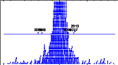
ANOVA Table for ROE by ANNEE
|
Source
|
Sum of Squares
|
Df
|
Mean Square
|
F-Ratio
|
P-Value
|
|
Between groups
|
5,2512
|
4
|
1,3128
|
4,24
|
0,0020
|
|
Within groups
|
878,206
|
2835
|
0,309773
|
|
|
|
Total (Corr.)
|
883,457
|
2839
|
|
|
|
The StatAdvisor
The ANOVA table decomposes the variance of ROE into two
components: a between-group component and a within-group component. The
F-ratio, which in this case equals 4,23794, is a ratio of the between-group
estimate to the within-group estimate. Since the P-value of the F-test is less
than 0,05, there is a statistically significant difference between the mean ROE
from one level of ANNEE to another at the 95,0% confidence level. To determine
which means are significantly different from which others, select Multiple
Range Tests from the list of Tabular Options.
ANOVA for ROE


2
Table of Means for ROE by ANNEE with 90,0 percent LSD
intervals
0,04
|
|
|
Stnd. error
|
|
|
|
ANNEE
|
Count
|
Mean
|
(pooled s)
|
Lower limit
|
Upper limit
|
|
0
2006
|
568
|
-0,0079864
|
0,0233533
|
-0,0351483
|
0,0191755
|
|
2007
|
568
|
0,0882099
|
0,0233533
|
0,061048
|
0,115372
|
|
2008
004
|
568
|
0,07103
|
0,0233533
|
0,043868
|
0,0981919
|
|
2009
|
568
|
0,00166802
2007
|
,233533
2008 2
|
-0,0254939
2010
|
0,0288299
|
|
2010
|
568
|
0,0906529
|
0,0233533
NNEE
|
0,063491
|
0,117815
|
|
Total
|
2840
|
0,0487149
|
|
|
|
The StatAdvisor
This table shows the mean ROE for each level of ANNEE. It also
shows the standard error of each mean, which is a measure of its sampling
variability. The standard error is formed by dividing the pooled standard
deviation by the square root of the number of observations at each level. The
table also displays an interval around each mean. The intervals currently
displayed are based on Fisher's least significant difference (LSD) procedure.
They are constructed in such a way that if two means are the same, their
intervals will overlap 95,0% of the time. You can display the intervals
graphically by selecting Means Plot from the list of Graphical Options. In the
Multiple Range Tests, these intervals are used to determine which means are
significantly different from which others.
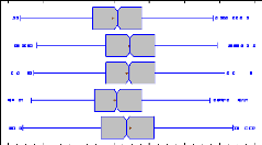
Multiple Range Tests for ROE by ANNEE Method:
90,0 percent LSD
|
ANNEE
|
Count
|
Mean
|
Homogeneous Groups
|
|
2006
|
568
|
-0,0079864
|
X
|
|
2009
|
568
|
0,00166802
|
X
|
|
2008
|
568
|
0,07103
|
X
|
|
2007
|
568
|
0,0882099
|
X
|
|
2010
|
568
|
Box-
0,0906529
|
W h
X
|
|
Contrast
|
Sig.
|
Difference
|
+/- Limits
|
|
2006 - 2007
2006
|
*
|
-0,0961963
|
0,0543239
|
|
2006 - 2008
|
*
|
-0,0790164
|
0,0543239
|
|
2006 - 2009
|
|
-0,00965442
|
0,0543239
|
|
2007
2006 - 2010
|
*
|
-0,0986393
|
0,0543239
|
|
2007 - 2008
|
|
0,0171799
|
0,0543239
|
|
2008
2007 - 2009
|
*
|
0,0865419
|
0,0543239
|
|
2007 - 2010
|
|
-0,00244305
|
0,0543239
|
|
28 - 2009
2009
|
*
|
0,0693619
|
0,0543239
|
|
2008 - 2010
|
|
-0,019623
|
0,0543239
|
|
2009 - 2010
2010
|
*
|
-0,0889849
|
0,0543239
|
* denotes a statistically significant difference.
The StatAdvisor
This table applies a multiple comparison procedure to determine
which means are significantly different from which others. The bottom half of
the output shows the estimated difference between each pair of means. An
asterisk has been placed next to 6 pairs, indicating that these pairs show
statistically significant differences at the 95,0% confidence level. At the top
of the page, 2 homogenous groups are identified using columns of X's. Within
each column, the levels containing X's form a group of means within which there
are no statistically significant differences. The method currently being used
to discriminate among the means is Fisher's least significant difference (LSD)
procedure. With this method, there is a 5,0% risk of calling each pair of means
significantly different when the actual difference equals 0.
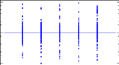
Variance Check
|
Test
|
P-Value
|
|
Levene's
|
1,56665
|
0,180425
|
|
Comparison
|
Sigma1
|
Sigma2
|
F-Ratio
|
P-Value
|
|
2006 / 2007
|
0,541224
|
0,498518
|
1,17867
|
0,0506
|
|
2006 / 2008
|
0,541224
|
0,60985
|
0,787605
|
0,0045
|
|
2006 / 2009
|
0,541224
|
0,489926
|
1,22038
|
0,0179
|
|
2006 / 2010
|
0,541224
|
0,628869
|
0,740685
|
0,0004
|
|
2007 / 2008
|
0,498518
|
0,60985
|
0,668216
|
0,0000
|
|
2007 / 2009
|
0,498518
|
0,489926
|
1,03539
|
0,6790
|
|
2007 / 2010
|
0,498518
|
0,628869
|
0,628409
|
0,0000
|
|
2008 / 2009
|
0,60985
|
0,489926
|
1,54948
|
0,0000
|
|
2008 / 2010
|
0,60985
|
0,628869
|
0,940428
|
0,4649
|
|
2009 / 2010
|
0,489926
|
0,628869
|
0,606932
|
0,0000
|
The StatAdvisor
The statistic displayed in this table tests the null hypothesis
that the standard deviations of ROE within each of the 5 levels of
4
ANNEE is the same. Of particular interest is the P-value. Since
the P-value is greater than or equal to 0,05, there is not a
statistically significant difference amongst the standard
deviations at the 95,0% confidence level.
The table also shows a comparison of the standard deviations for
each pair of samples. P-Values below 0.05, of which there are 7, indicate a
statistically significant difference between the two sigmas at the 5%
significance level.
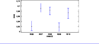
Kruskal-Wallis Test for ROE by ANNEE
|
ANNEE
|
Sample Size
|
Average Rank
|
|
2006
|
568
|
1275,31
|
|
2007
|
568
|
1547,93
|
|
2008
|
568
|
1517,84
|
|
2009
|
568
|
1287,11
|
|
2010
|
568
|
1474,32
|
Test statistic = 57,0073 P-Value = 1,2328E-11
The StatAdvisor
The Kruskal-Wallis test tests the null hypothesis that the
medians of ROE within each of the 5 levels of ANNEE are the same. The data from
all the levels is first combined and ranked from smallest to largest. The
average rank is then computed for the data at each level. Since the P-value is
less than 0,05, there is a statistically significant difference amongst the
medians at the 95,0% confidence level. To determine which medians are
significantly different from which others, select Box-and-Whisker Plot from the
list of Graphical Options and select the median notch option.
Mood's Median Test for ROE by ANNEE Total n =
2840
Grand median = 0,0583012
0,12
|
0,1
ANNEE
|
Sample Size
|
n<=
|
n>
|
Median
|
90,0% lower CL
|
90,0% upper CL
|
|
2006
|
568
|
326
|
242
|
0,0195117
|
0,00305438
|
0,041546
|
|
0,08
2007
|
568
|
245
|
323
|
0,0910952
|
0,0759334
|
0,110756
|
|
2008
|
568
|
250
|
318
|
0,0837851
|
0,065602
|
0,0957051
|
|
0,06
2009
|
568
|
328
|
240
|
0,0176906
|
0,00193535
|
0,0337506
|
|
2010
004
|
568
|
271
|
297
|
0,0734001
|
0,0512998
|
0,091961
|
Test statistic = 46,0986 P-Value = 2,3492E-9
The StatAdvisor
Mood's median test tests the hypothesis that the medians of all 5
samples are equal. It does so by counting the number of
0
observations in each sample on either side of the grand median,
which equals 0,0583012. Since the P-value for the chi-
2006 2007 2008 2009 2010
square test is less than 0,1, the medians of the samples are
significantly different at the 90,0% confidence level. Also
ANNEE
included (if available) are 90,0% confidence intervals for each
median based on the order statistics of each sample.
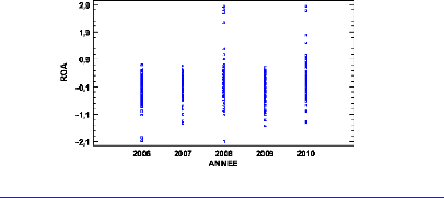
Appendix 7:ROA by year
One-Way ANOVA - ROA by ANNEE
Dependent variable: ROA Factor: ANNEE
Number of observations: 2840 Number of levels: 5
The StatAdvisor
This procedure performs a one-way analysis of variance for ROA.
It constructs various tests and graphs to compare the mean values of ROA for
the 5 different levels of ANNEE. The F-test in the ANOVA table will test
whether there are any significant differences amongst the means. If there are,
the Multiple Range Tests will tell you which means are significantly different
from which others. If you are worried about the presence of outliers, choose
the Kruskal-Wallis Test which compares medians instead of means. The various
plots will help you judge the practical significance of the results, as well as
allow you to look for possible violations of the assumptions underlying the
analysis of variance.
Summary Statistics for ROA
|
ANNEE
|
Count
|
Average
|
Standard deviation
|
Coeff. of variation
|
Minimum
|
Maximum
|
Range
|
Stnd. skewness
|
|
2006
|
568
|
-0,013372
|
0,223258
|
-1669,59%
|
-2,05464
|
0,701545
|
2,75619
|
-31,7124
|
|
2007
|
568
|
0,045657
|
0,198647
|
435,086%
|
-1,41503
|
0,677594
|
2,09262
|
-20,8092
|
|
2008
|
568
|
Scatte
0,0677319
|
by Level
0,328621
|
485,179%
|
-2,07651
|
2,83152
|
4,90803
|
33,4605
|
|
2009
|
568
|
-0,0042941
|
0,204192
|
-4755,18%
|
-1,50563
|
0,600911
|
2,10654
|
-23,9402
|
|
2,9
2010
|
568
|
0,0572362
|
0,292304
|
510,697%
|
-1,41254
|
2,82314
|
4,23567
|
28,9587
|
|
Total
|
2840
|
0,0305918
|
0,256688
|
839,075%
|
-2,07651
|
2,83152
|
4,90803
|
33,8379
|
|
ANNEE
|
Stnd. kurtosis
|
|
2006
|
118,296
|
|
0,9
2007
|
63,4508
|
|
2008
|
169,523
|
|
-0,1
209
|
65,4003
|
|
2010
|
147,887
|
|
-1,1
Total
|
386,057
|
The StatAdvisor
21
This table shows various statistics for ROA for each of the 5
levels of ANNEE. The one-way analysis of variance is
2006 2007 2008 2009 2010
primarily intended to compare the means of the different levels,
listed here under the Average column. Select Means Plot
ANNEE
from the list of Graphical Options to display the means
graphically.
WARNING: The standardized skewness and/or kurtosis is outside the
range of -2 to +2 for 5 levels of ANNEE. This indicates some significant
nonnormality in the data, which violates the assumption that the data come from
normal distributions. You may wish to transform the data or use the
Kruskal-Wallis test to compare the medians instead of the means.
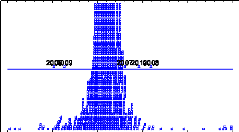
ANOVA Table for ROA by ANNEE
|
Source
|
Sum of Squares
|
Df
|
Mean Square
|
F-Ratio
|
P-Value
|
|
Between groups
|
3,10475
|
4
|
0,776188
|
11,96
|
0,0000
|
|
Within groups
|
183,953
|
2835
|
0,0648865
|
|
|
|
Total (Corr.)
|
187,058
|
2839
|
|
|
|
The StatAdvisor
The ANOVA table decomposes the variance of ROA into two
components: a between-group component and a within-group component. The
F-ratio, which in this case equals 11,9622, is a ratio of the between-group
estimate to the within-group estimate. Since the P-value of the F-test is less
than 0,05, there is a statistically significant difference between the mean ROA
from one level of ANNEE to another at the 95,0% confidence level. To determine
which means are significantly different from which others, select Multiple
Range Tests from the list of Tabular Options.
ANOVA for ROA
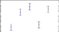
0,2 0,8 1,
Table of Means for ROA by ANNEE with 90,0 percent LSD
intervals
0,03
|
|
|
Stnd. error
|
|
|
|
0,01
ANNEE
|
Count
|
Mean
|
(pooled s)
|
Lower limit
|
Upper limit
|
|
2006
0,01
|
568
|
-0,013372
|
0,0106882
|
-0,0258033
|
-0,000940728
|
|
2007
|
568
|
0,045657
|
0,0106882
|
0,0332257
|
0,0580883
|
|
2008
003
|
568
|
0,0677319
|
0,0106882
|
0,0553006
|
0,0801632
|
|
2009
|
568
|
-0,0042941
2007
|
0,106882
2008 2
|
-0,0167254
2010
|
0,00813719
|
|
2010
|
568
|
0,0572362
|
0,0106882
NNEE
|
0,0448049
|
0,0696675
|
|
Total
|
2840
|
0,0305918
|
|
|
|
The StatAdvisor
This table shows the mean ROA for each level of ANNEE. It also
shows the standard error of each mean, which is a measure of its sampling
variability. The standard error is formed by dividing the pooled standard
deviation by the square root of the number of observations at each level. The
table also displays an interval around each mean. The intervals currently
displayed are based on Fisher's least significant difference (LSD) procedure.
They are constructed in such a way that if two means are the same, their
intervals will overlap 95,0% of the time. You can display the intervals
graphically by selecting Means Plot from the list of Graphical Options. In the
Multiple Range Tests, these intervals are used to determine which means are
significantly different from which others.
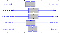
Multiple Range Tests for ROA by ANNEE Method:
90,0 percent LSD
|
ANNEE
|
Count
|
Mean
|
Homogeneous Groups
|
|
2006
|
568
|
-0,013372
|
X
|
|
2009
|
568
|
-0,0042941
|
X
|
|
2007
|
568
|
0,045657
|
X
|
|
2010
|
568
|
0,0572362
|
X
|
|
2008
|
568
|
Box-
0,0677319
|
X h
X
|
|
Contrast
|
Sig.
|
Difference
|
+/- Limits
|
|
2006 - 2007
2006
|
*
|
-0,059029
|
0,0248626
|
|
2006 - 2008
|
*
|
-0,0811039
|
0,0248626
|
|
2006 - 2009
|
|
-0,00907792
|
0,0248626
|
|
2007
2006 - 2010
|
*
|
-0,0706082
|
0,0248626
|
|
2007 - 2008
|
|
-0,0220748
|
0,0248626
|
|
2008
2007 - 2009
|
*
|
0,0499511
|
0,0248626
|
|
2007 - 2010
|
|
-0,0115791
|
0,0248626
|
|
28 - 2009
2009
|
*
|
0,072026
|
0,0248626
|
|
2008 - 2010
|
|
0,0104957
|
0,0248626
|
|
2009 - 2010
2010
|
*
|
-0,0615303
|
0,0248626
|
* denotes a statistically significant difference.
The StatAdvisor
This table applies a multiple comparison procedure to determine
which means are significantly different from which others. The bottom half of
the output shows the estimated difference between each pair of means. An
asterisk has been placed next to 6 pairs, indicating that these pairs show
statistically significant differences at the 95,0% confidence level. At the top
of the page, 2 homogenous groups are identified using columns of X's. Within
each column, the levels containing X's form a group of means within which there
are no statistically significant differences. The method currently being used
to discriminate among the means is Fisher's least significant difference (LSD)
procedure. With this method, there is a 5,0% risk of calling each pair of means
significantly different when the actual difference equals 0.
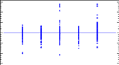
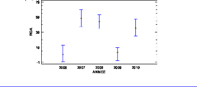
Variance Check
|
Test
|
P-Value
|
|
Levene's
|
2,58661
|
0,0352025
|
|
Comparison
|
Sigma1
|
Sigma2
|
F-Ratio
|
P-Value
|
|
2006 / 2007
|
0,223258
|
0,198647
|
1,26314
|
0,0055
|
|
2006 / 2008
|
0,223258
|
0,328621
|
0,461557
|
0,0000
|
|
2006 / 2009
|
0,223258
|
0,204192
|
1,19546
|
0,0337
|
|
2006 / 2010
|
0,223258
|
0,292304
|
0,583375
|
0,0000
|
|
2007 / 2008
|
0,198647
|
0,328621
|
0,365405
|
0,0000
|
|
2007 / 2009
|
0,198647
|
0,204192
|
0,946424
|
0,5123
|
|
2007 / 2010
|
0,198647
|
0,292304
|
0,461846
|
0,0000
|
|
2008 / 2009
|
0,328621
|
0,204192
|
2,59007
|
0,0000
|
|
2008 / 2010
|
0,328621
|
0,292304
|
1,26393
|
0,0054
|
|
2009 / 2010
|
0,204192
|
0,292304
|
0,48799
|
0,0000
|
The StatAdvisor
The statistic displayed in this table tests the null hypothesis
that the standard deviations of ROA within each of the 5 levels of
3
ANNEE is the same. Of particular interest is the P-value. Since
the the P-value is less than 0,05, there is a statistically significant
difference amongst the standard deviations at the 95,0% confidence level. This
violates one of the important
2
assumptions underlying the analysis of variance and will
invalidate most of the standard statistical tests.
The table also shows a comparison of the standard deviations for
each pair of samples. P-Values below 0.05, of which there are 9, indicate a
statistically significant difference between the two sigmas at the 5%
significance level.
0
Kruskal-Wallis Test for ROA by ANNEE
|
ANNEE
|
Sample Size
|
Average Rank
|
|
2006
|
568
|
1253,72
|
|
2007
|
568
|
1552,39
|
|
2008
|
568
|
1545,22
|
|
2009
|
568
|
1269,77
|
|
2010
|
568
|
1481,39
|
Test statistic = 73,6591 P-Value = 0
The StatAdvisor
The Kruskal-Wallis test tests the null hypothesis that the
medians of ROA within each of the 5 levels of ANNEE are the same. The data from
all the levels is first combined and ranked from smallest to largest. The
average rank is then computed for the data at each level. Since the P-value is
less than 0,05, there is a statistically significant difference amongst the
medians at the 95,0% confidence level. To determine which medians are
significantly different from which others, select Box-and-Whisker Plot from the
list of Graphical Options and select the median notch option.
Mood's Median Test for ROA by ANNEE Total n =
2840
0001
Grand median = 0,034619
79
|
ANNEE
|
Sample Size
|
n<=
|
n>
|
Median
|
90,0% lower CL
|
90,0% upper CL
|
|
59
2006
|
568
|
339
|
229
|
0,00945275
|
-0,000555481
|
0,0218933
|
|
2007
|
568
|
242
|
326
|
0,0570648
|
0,0460463
|
0,0689174
|
|
2008
|
568
|
248
|
320
|
0,0528593
|
0,0436125
|
0,0621654
|
|
39
2009
|
568
|
327
|
241
|
0,0121847
|
0,000872383
|
0,0184358
|
|
2010
|
568
|
264
|
304
|
0,044225
|
0,0338877
|
0,0561194
|
Test statistic = 58,6901 P-Value = 5,46618E-12
19
The StatAdvisor
Mood's median test tests the hypothesis that the medians of all 5
samples are equal. It does so by counting the number of
1
observations in each sample on either side of the grand median,
which equals 0,034619. Since the P-value for the chi-square
2006 2007 2008 2009 2010
test is less than 0,1, the medians of the samples are
significantly different at the 90,0% confidence level. Also included (if
ANNEE
available) are 90,0% confidence intervals for each median based
on the order statistics of each sample.
Appendix 8: ROE by groups for dairy
production
One-Way ANOVA - ROE by Groups
(ANNEE=2010&SPECIALISATION="Bovins lait")
Dependent variable: ROE
Factor: Groups
Selection variable: ANNEE=2010&SPECIALISATION="Bovins
lait"
Number of observations: 141 Number of levels: 5
Summary Statistics for ROE
|
Groups
|
Count
|
Average
|
Standard deviation
|
Coeff. of variation
|
Minimum
|
Maximum
|
Range
|
Stnd. skewness
|
|
1
|
10
|
-0,0069795
|
0,262229
|
-3757,13%
|
-0,484615
|
0,252975
|
0,73759
|
-1,14121
|
|
2
|
48
|
0,142481
|
0,180874
|
126,946%
|
-0,412968
|
0,474718
|
0,887686
|
-2,98642
|
|
3
|
43
|
0,123011
|
0,208889
|
169,813%
|
-0,37387
|
0,642566
|
1,01644
|
0,773958
|
|
4
|
28
|
0,0362009
|
0,195441
|
539,878%
|
-0,268354
|
0,67475
|
0,943103
|
2,75521
|
|
5
|
12
|
0,0452324
|
0,0883501
|
195,325%
|
-0,0649112
|
0,241946
|
0,306857
|
1,52055
|
|
Total
|
141
|
0,0965617
|
0,197818
|
204,861%
|
-0,484615
|
0,67475
|
1,15936
|
-0,42451
|
|
Groups
|
Stnd. kurtosis
|
|
1
|
-0,367154
|
|
2
|
2,91906
|
|
3
|
0,924502
|
|
4
|
3,11992
|
|
5
|
0,672821
|
|
Total
|
2,31948
|
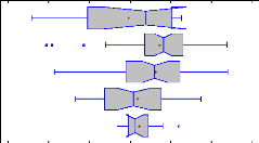
Kruskal-Wallis Test for ROE by Groups
|
Groups
|
Sample Size
|
Average Rank
|
|
2
1
|
10
|
59,3
|
|
2
Cs)
|
48
|
83,875
|
|
3
|
43
|
75,2093
|
|
4
|
28
|
53,7857
|
|
5
|
12
|
54,3333
|
Test statistic = 13,0166 P-Value = 0,0111951
Mood's Median Test for ROE by Groups Total n =
141
6 04
Grand median = 0,104137
|
Groups
|
Sample Size
|
n<=
|
n>
|
Median
|
90,0% lower CL
|
90,0% upper CL
|
|
1
|
10
|
6
|
4
|
0,0749859
|
-0,379136
|
0,23285
|
|
2
|
48
|
17
|
31
|
0,162987
|
0,111378
|
0,214087
|
|
3
|
43
|
20
|
23
|
0,121517
|
0,0528025
|
0,196325
|
|
4
|
28
|
19
|
9
|
0,0175846
|
-0,083556
|
0,106835
|
|
5
|
12
|
9
|
3
|
0,0220671
|
-0,0257561
|
0,128591
|
Test statistic = 11,2575 P-Value = 0,0238171
One-Way ANOVA - ROE by Groups
(ANNEE=2009&SPECIALISATION="Bovins lait")
Dependent variable: ROE
Factor: Groups
Selection variable: ANNEE=2009&SPECIALISATION="Bovins
lait"
Number of observations: 141 Number of levels: 5
Summary Statistics for ROE
|
Groups
|
Count
|
Average
|
Standard deviation
|
Coeff. of variation
|
Minimum
|
Maximum
|
Range
|
Stnd. skewness
|
|
1
|
10
|
-0,17879
|
1,37918
|
-771,394%
|
-3,68929
|
1,89707
|
5,58636
|
-2,33501
|
|
2
|
42
|
0,11621
|
0,185857
|
159,932%
|
-0,376288
|
0,596295
|
0,972584
|
0,502
|
|
3
|
39
|
0,0630057
|
0,137776
|
218,672%
|
-0,181477
|
0,29342
|
0,474897
|
-0,76982
|
|
4
|
36
|
0,0100035
|
0,175893
|
1758,32%
|
-0,318248
|
0,462527
|
0,780774
|
2,18408
|
|
5
|
14
|
-0,0197315
|
0,0917217
|
-464,848%
|
-0,213078
|
0,123559
|
0,336637
|
-0,648606
|
|
Total
|
141
|
0,0399575
|
0,389822
|
975,59%
|
-3,68929
|
1,89707
|
5,58636
|
-26,7144
|
|
Groups
|
Stnd. kurtosis
|
|
1
|
3,83774
|
|
2
|
1,17713
|
|
3
|
-1,46433
|
|
4
|
0,88851
|
|
5
|
0,0493783
|
|
Total
|
153,54
|
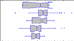
Kruskal-Wallis Test for ROE by Groups
|
Groups
3
|
Sample Size
|
Average Rank
|
|
1
|
10
|
65,2
|
|
2
|
42
|
85,5952
|
|
3
|
39
|
76,3077
|
|
4
|
36
|
57,1389
|
|
5
|
14
|
52,2143
|
Test statistic = 13,3289 P-Value = 0,00977558 Mood's
Median Test for ROE by Groups
ROE
Total n = 141
Grand median = 0,0435052
|
Groups
|
Sample Size
|
n<=
|
n>
|
Median
|
90,0% lower CL
|
90,0% upper CL
|
|
1
|
10
|
5
|
5
|
0,0550638
|
-0,618245
|
0,387143
|
|
2
|
42
|
13
|
29
|
0,099151
|
0,0719154
|
0,155127
|
|
3
|
39
|
16
|
23
|
0,0898162
|
0,0108911
|
0,150199
|
|
4
|
36
|
26
|
10
|
-0,00936615
|
-0,0647502
|
0,0233567
|
|
5
|
14
|
11
|
3
|
-0,0151896
|
-0,103506
|
0,0445331
|
Test statistic = 19,0281 P-Value = 0,000776032
One-Way ANOVA - ROE by Groups
(ANNEE=2008&SPECIALISATION="Bovins lait")
Dependent variable: ROE
Factor: Groups
Selection variable: ANNEE=2008&SPECIALISATION="Bovins
lait"
Number of observations: 141 Number of levels: 5
Summary Statistics for ROE
|
Groups
|
Count
|
Average
|
Standard deviation
|
Coeff. of variation
|
Minimum
|
Maximum
|
Range
|
Stnd. skewness
|
|
1
|
6
|
0,075066
|
2,21034
|
2944,52%
|
-3,267
|
3,703
|
6,97
|
0,288721
|
|
2
|
33
|
0,106858
|
0,284379
|
266,127%
|
-1,04792
|
0,891704
|
1,93962
|
-3,53472
|
|
3
|
48
|
0,103257
|
0,150159
|
145,423%
|
-0,177508
|
0,584271
|
0,761778
|
2,14386
|
|
4
|
40
|
0,0920779
|
0,125932
|
136,767%
|
-0,156094
|
0,329752
|
0,485846
|
-0,006572
|
|
5
|
14
|
0,121409
|
0,358122
|
294,972%
|
-0,115502
|
1,34073
|
1,45623
|
5,31902
|
|
Total
|
141
|
0,101531
|
0,4658
|
458,776%
|
-3,267
|
3,703
|
6,97
|
3,27998
|
|
Groups
|
Stnd. kurtosis
|
|
1
|
1,24469
|
|
2
|
10,951
|
|
3
|
1,51367
|
|
4
|
-0,748698
|
|
5
|
9,66003
|
|
Total
|
108,366
|
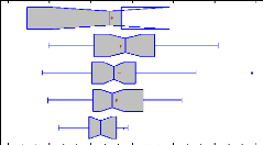
Kruskal-Wallis Test for ROE by Groups
3
|
Groups
|
Sample Size
|
Average Rank
|
|
1
|
6
|
58,1667
|
|
2
|
33
|
79,0303
|
|
3
|
48
|
71,7083
|
|
4
|
40
|
70,575
|
|
5
|
14
|
56,3571
0
, ,
|
Test statistic = 3,68552 P-Value = 0,450235
ROE
Mood's Median Test for ROE by Groups Total n =
141
Grand median = 0,0900887
|
Groups
|
Sample Size
|
n<=
|
n>
|
Median
|
90,0% lower CL
|
90,0% upper CL
|
|
1
|
6
|
3
|
3
|
0,0677642
|
|
|
|
2
|
33
|
11
|
22
|
0,125305
|
0,0811245
|
0,185447
|
|
3
|
48
|
25
|
23
|
0,0847578
|
0,0506366
|
0,131847
|
|
4
|
40
|
22
|
18
|
0,0781741
|
0,0264757
|
0,146814
|
|
5
|
14
|
10
|
4
|
0,0356748
|
-0,0276925
|
0,118881
|
Test statistic = 6,71467 P-Value = 0,151757
One-Way ANOVA - ROE by Groups
(ANNEE=2007&SPECIALISATION="Bovins lait")
Dependent variable: ROE
Factor: Groups
Selection variable: ANNEE=2007&SPECIALISATION="Bovins
lait"
Number of observations: 141 Number of levels: 5
Summary Statistics for ROE
|
Groups
|
Count
|
Average
|
Standard deviation
|
Coeff. of variation
|
Minimum
|
Maximum
|
Range
|
Stnd. skewness
|
|
1
|
7
|
-0,20666
|
1,02638
|
-496,653%
|
-2,52135
|
0,386503
|
2,90785
|
-2,79018
|
|
2
|
34
|
0,177157
|
0,250627
|
141,472%
|
-0,362507
|
1,06101
|
1,42352
|
3,11097
|
|
3
|
49
|
0,0841043
|
0,146422
|
174,096%
|
-0,481832
|
0,37319
|
0,855022
|
-3,64391
|
|
4
|
38
|
0,0371798
|
0,147275
|
396,114%
|
-0,270465
|
0,39789
|
0,668355
|
0,0203899
|
|
5
|
13
|
-0,0100111
|
0,0819924
|
-819,015%
|
-0,105939
|
0,165918
|
0,271857
|
1,15795
|
|
Total
|
141
|
0,0707839
|
0,28493
|
402,535%
|
-2,52135
|
1,06101
|
3,58236
|
-24,7291
|
|
Groups
|
Stnd. kurtosis
|
|
1
|
3,6496
|
|
2
|
5,01567
|
|
3
|
4,98283
|
|
4
|
0,0175206
|
|
5
|
0,00589768
|
|
Total
|
120,25
|
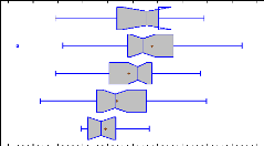
Kruskal-Wallis Test for ROE by Groups
4
|
Groups
|
Sample Size
|
Average Rank
|
|
1
|
7
|
84,1429
|
|
2
|
34
|
87,8529
|
|
3
|
49
|
74,4898
|
|
4
|
38
|
1 0
59,1053
|
|
5
|
13
|
41,4615
|
Test statistic = 16,8905 P-Value = 0,00202995
Mood's Median Test for ROE by Groups Total n =
141
Grand median = 0,0919618
|
Groups
|
Sample Size
|
n<=
|
n>
|
Median
|
90,0% lower CL
|
90,0% upper CL
|
|
1
|
7
|
2
|
5
|
0,1569
|
|
|
|
2
|
34
|
10
|
24
|
0,140842
|
0,102307
|
0,193956
|
|
3
|
49
|
23
|
26
|
0,120696
|
0,0469401
|
0,164298
|
|
4
|
38
|
24
|
14
|
0,0287984
|
-0,0153515
|
0,119707
|
|
5
|
13
|
12
|
1
|
-0,0275842
|
-0,0825783
|
0,0486049
|
Test statistic = 19,1672 P-Value = 0,000728654
One-Way ANOVA - ROE by Groups
(ANNEE=2006&SPECIALISATION="Bovins lait")
Dependent variable: ROE
Factor: Groups
Selection variable: ANNEE=2006&SPECIALISATION="Bovins
lait"
Number of observations: 141 Number of levels: 5
Summary Statistics for ROE
|
Groups
|
Count
|
Average
|
Standard deviation
|
Coeff. of variation
|
Minimum
|
Maximum
|
Range
|
Stnd. skewness
|
|
1
|
8
|
-0,143292
|
0,641699
|
-447,826%
|
-1,38481
|
0,676675
|
2,06148
|
-1,25734
|
|
2
|
35
|
0,0225383
|
0,240142
|
1065,48%
|
-1,09395
|
0,276005
|
1,36996
|
-7,54682
|
|
3
|
50
|
0,0475295
|
0,194926
|
410,116%
|
-0,699781
|
0,443904
|
1,14368
|
-3,02011
|
|
4
|
34
|
0,00565164
|
0,126919
|
2245,71%
|
-0,254159
|
0,257111
|
0,511269
|
0,526975
|
|
5
|
14
|
0,0271876
|
0,10212
|
375,611%
|
-0,0965745
|
0,303625
|
0,4002
|
2,70992
|
|
Total
|
141
|
0,0183813
|
0,233466
|
1270,13%
|
-1,38481
|
0,676675
|
2,06148
|
-12,3857
|
|
Groups
|
Stnd. kurtosis
|
|
1
|
0,679283
|
|
2
|
16,2943
|
|
3
|
4,88459
|
|
4
|
-0,227566
|
|
5
|
2,80584
|
|
Total
|
31,5881
|
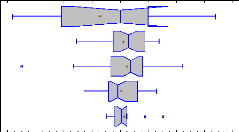
Kruskal-Wallis Test for ROE by Groups
|
Groups
5
|
Sample Size
|
Average Rank
|
|
1
|
8
|
67,5
|
|
2
|
35
|
76,2286
-02
|
|
3
|
50
|
75,86
|
|
4
|
34
|
61,1471
|
|
5
|
14
|
66,5
|
Test statistic = 3,48819 P-Value = 0,479676
Mood's Median Test for ROE by Groups Total n =
141
Grand median = 0,0333134
|
Groups
|
Sample Size
|
n<=
|
n>
|
Median
|
90,0% lower CL
|
90,0% upper CL
|
|
1
|
8
|
5
|
3
|
-0,000383141
|
-1,3004
|
0,615859
|
|
2
|
35
|
14
|
21
|
0,0600382
|
-0,0171497
|
0,142537
|
|
3
|
50
|
20
|
30
|
0,0771671
|
0,00399078
|
0,126858
|
|
4
|
34
|
22
|
12
|
-0,0159893
|
-0,0583432
|
0,0413279
|
|
5
|
14
|
10
|
4
|
0,0124171
|
-0,0434617
|
0,0456193
|
Test statistic = 9,40599 P-Value = 0,0517153
Appendix 9: ROE by groups for cattle
specialization
One-Way ANOVA - ROE by Groups
(ANNEE=2006&SPECIALISATION="Bovins viande")
Dependent variable: ROE
Factor: Groups
Selection variable: ANNEE=2006&SPECIALISATION="Bovins
viande"
Number of observations: 45 Number of levels: 5
Summary Statistics for ROE
|
Groups
|
Count
|
Average
|
Standard deviation
|
Coeff. of variation
|
Minimum
|
Maximum
|
Range
|
Stnd. skewness
|
|
1
|
7
|
-0,0824401
|
0,59067
|
-716,484%
|
-1,40816
|
0,248772
|
1,65693
|
-2,73727
|
|
2
|
6
|
-0,133896
|
0,230839
|
-172,402%
|
-0,567189
|
0,0267818
|
0,593971
|
-1,70149
|
|
3
|
7
|
-0,100753
|
0,239325
|
-237,537%
|
-0,526313
|
0,16275
|
0,689062
|
-1,00633
|
|
4
|
16
|
-0,158071
|
0,283015
|
-179,042%
|
-1,0385
|
0,149503
|
1,188
|
-3,41863
|
|
5
|
9
|
-0,138262
|
0,411863
|
-297,886%
|
-1,21844
|
0,131187
|
1,34963
|
-3,43557
|
|
Total
|
45
|
-0,130205
|
0,34697
|
-266,48%
|
-1,40816
|
0,248772
|
1,65693
|
-6,25348
|
|
Groups
|
Stnd. kurtosis
|
|
1
|
3,53339
|
|
2
|
1,45072
|
|
3
|
0,225223
|
|
4
|
4,876
|
|
5
|
5,01709
|
|
Total
|
7,65586
|
Kruskal-Wallis Test for ROE by Groups
|
Groups
|
Sample Size
|
Average Rank
|
|
1
|
7
|
33,7143
|
|
2
|
6
|
20,6667
|
|
3
|
7
|
22,2857
|
|
4
|
16
|
19,1875
|
|
5
|
9
|
23,5556
|
Test statistic = 6,23275 P-Value = 0,182427
Mood's Median Test for ROE by Groups Total n =
45
Grand median = -0,0364259
|
Groups
|
Sample Size
|
n<=
|
n>
|
Median
|
90,0% lower CL
|
90,0% upper CL
|
|
1
|
7
|
1
|
6
|
0,149788
|
|
|
|
2
|
6
|
3
|
3
|
-0,0463576
|
|
|
|
3
|
7
|
4
|
3
|
-0,0429657
|
|
|
|
4
|
16
|
10
|
6
|
-0,0797749
|
-0,286345
|
0,0373879
|
|
5
|
9
|
5
|
4
|
-0,0364259
|
-0,719997
|
0,122984
|
Test statistic = 4,80555 P-Value = 0,307838
One-Way ANOVA - ROE by Groups
(ANNEE=2007&SPECIALISATION="Bovins viande")
Dependent variable: ROE
Factor: Groups
Selection variable: ANNEE=2007&SPECIALISATION="Bovins
viande"
Number of observations: 45 Number of levels: 5
Summary Statistics for ROE
|
Groups
|
Count
|
Average
|
Standard deviation
|
Coeff. of variation
|
Minimum
|
Maximum
|
Range
|
Stnd. skewness
|
|
1
|
5
|
0,350147
|
0,452136
|
129,127%
|
-0,0783535
|
0,965862
|
1,04422
|
0,501517
|
|
2
|
4
|
0,0319552
|
0,274144
|
857,902%
|
-0,374624
|
0,203506
|
0,57813
|
-1,52757
|
|
3
|
10
|
-0,00885641
|
0,230547
|
-2603,16%
|
-0,436945
|
0,272862
|
0,709807
|
-1,60867
|
|
4
|
14
|
-0,0810269
|
0,28336
|
-349,711%
|
-1,03602
|
0,134314
|
1,17033
|
-5,12914
|
|
5
|
12
|
-0,119093
|
0,347957
|
-292,173%
|
-1,08706
|
0,167536
|
1,25459
|
-3,22219
|
|
Total
|
45
|
-0,0171888
|
0,329044
|
-1914,29%
|
-1,08706
|
0,965862
|
2,05292
|
-2,20465
|
|
Groups
|
Stnd. kurtosis
|
|
1
|
-0,792416
|
|
2
|
1,43611
|
|
3
|
0,476563
|
|
4
|
9,17569
|
|
5
|
3,97617
|
|
Total
|
6,68529
|
Kruskal-Wallis Test for ROE by Groups
|
Groups
|
Sample Size
|
Average Rank
|
|
1
|
5
|
31,0
|
|
2
|
4
|
30,25
|
|
3
|
10
|
26,1
|
|
4
|
14
|
18,1429
|
|
5
|
12
|
20,3333
|
Test statistic = 6,0404 P-Value = 0,196151
Mood's Median Test for ROE by Groups Total n =
45
Grand median = 0,0260234
|
Groups
|
Sample Size
|
n<=
|
n>
|
Median
|
90,0% lower CL
|
90,0% upper CL
|
|
1
|
5
|
2
|
3
|
0,250584
|
|
|
|
2
|
4
|
1
|
3
|
0,149469
|
|
|
|
3
|
10
|
3
|
7
|
0,0563751
|
-0,408074
|
0,18652
|
|
4
|
14
|
10
|
4
|
-0,0117706
|
-0,0781489
|
0,0366616
|
|
5
|
12
|
7
|
5
|
0,0195701
|
-0,364224
|
0,0845263
|
Test statistic = 5,68535 P-Value = 0,223911
One-Way ANOVA - ROE by Groups
(ANNEE=2008&SPECIALISATION="Bovins viande")
Dependent variable: ROE
Factor: Groups
Selection variable: ANNEE=2008&SPECIALISATION="Bovins
viande"
Number of observations: 45 Number of levels: 5
Summary Statistics for ROE
|
Groups
|
Count
|
Average
|
Standard deviation
|
Coeff. of variation
|
Minimum
|
Maximum
|
Range
|
Stnd. skewness
|
|
1
|
3
|
-0,137126
|
0,268858
|
-196,066%
|
-0,442407
|
0,0643751
|
0,506782
|
-1,04524
|
|
2
|
6
|
0,200511
|
0,0814852
|
40,6389%
|
0,124808
|
0,341432
|
0,216623
|
1,16574
|
|
3
|
12
|
0,193629
|
0,925176
|
477,808%
|
-0,481933
|
3,053
|
3,53493
|
4,4236
|
|
4
|
10
|
-0,0391609
|
0,0765327
|
-195,431%
|
-0,166521
|
0,0709146
|
0,237435
|
-0,429557
|
|
5
|
14
|
-0,233825
|
0,391322
|
-167,357%
|
-1,13931
|
0,081154
|
1,22046
|
-2,50106
|
|
Total
|
45
|
-0,0122204
|
0,546856
|
-4474,94%
|
-1,13931
|
3,053
|
4,19231
|
10,3766
|
|
Groups
|
Stnd. kurtosis
|
|
1
|
|
|
2
|
0,433379
|
|
3
|
7,37526
|
|
4
|
-0,621184
|
|
5
|
1,23119
|
|
Total
|
31,9128
|
Kruskal-Wallis Test for ROE by Groups
|
Groups
|
Sample Size
|
Average Rank
|
|
1
|
3
|
19,0
|
|
2
|
6
|
40,8333
|
|
3
|
12
|
24,6667
|
|
4
|
10
|
21,0
|
|
5
|
14
|
16,2143
|
Test statistic = 15,5023 P-Value = 0,0037652
Mood's Median Test for ROE by Groups Total n =
45
Grand median = -0,00954206
|
Groups
|
Sample Size
|
n<=
|
n>
|
Median
|
90,0% lower CL
|
90,0% upper CL
|
|
1
|
3
|
2
|
1
|
-0,0333468
|
|
|
|
2
|
6
|
0
|
6
|
0,177259
|
|
|
|
3
|
12
|
5
|
7
|
0,0251912
|
-0,299153
|
0,149681
|
|
4
|
10
|
6
|
4
|
-0,0288041
|
-0,128674
|
0,0316859
|
|
5
|
14
|
10
|
4
|
-0,0589653
|
-0,468499
|
0,0204429
|
Test statistic = 9,62062 P-Value = 0,0473268
One-Way ANOVA - ROE by Groups
(ANNEE=2009&SPECIALISATION="Bovins viande")
Dependent variable: ROE
Factor: Groups
Selection variable: ANNEE=2009&SPECIALISATION="Bovins
viande"
Number of observations: 45 Number of levels: 5
Summary Statistics for ROE
|
Groups
|
Count
|
Average
|
Standard deviation
|
Coeff. of variation
|
Minimum
|
Maximum
|
Range
|
Stnd. skewness
|
|
1
|
7
|
0,0674309
|
0,133599
|
198,127%
|
-0,0885807
|
0,339021
|
0,427602
|
1,678
|
|
2
|
6
|
-0,00554691
|
0,302544
|
-5454,28%
|
-0,536908
|
0,316999
|
0,853907
|
-1,1561
|
|
3
|
7
|
0,0118722
|
0,235413
|
1982,89%
|
-0,321133
|
0,434852
|
0,755984
|
0,734801
|
|
4
|
13
|
-0,0072047
|
0,257595
|
-3575,37%
|
-0,37133
|
0,729829
|
1,10116
|
2,94153
|
|
5
|
12
|
-0,204717
|
0,385528
|
-188,322%
|
-1,13015
|
0,0444478
|
1,1746
|
-2,77536
|
|
Total
|
45
|
-0,0450762
|
0,292856
|
-649,69%
|
-1,13015
|
0,729829
|
1,85998
|
-3,41959
|
|
Groups
|
Stnd. kurtosis
|
|
1
|
1,87505
|
|
2
|
0,748515
|
|
3
|
0,758146
|
|
4
|
4,36867
|
|
5
|
1,95883
|
|
Total
|
7,26813
|
Kruskal-Wallis Test for ROE by Groups
|
Groups
|
Sample Size
|
Average Rank
|
|
1
|
7
|
30,2857
|
|
2
|
6
|
26,1667
|
|
3
|
7
|
24,4286
|
|
4
|
13
|
21,3077
|
|
5
|
12
|
18,1667
|
Test statistic = 4,4266 P-Value = 0,35134
Mood's Median Test for ROE by Groups Total n =
45
Grand median = -0,030158
|
Groups
|
Sample Size
|
n<=
|
n>
|
Median
|
90,0% lower CL
|
90,0% upper CL
|
|
1
|
7
|
1
|
6
|
0,0295297
|
|
|
|
2
|
6
|
3
|
3
|
0,0492473
|
|
|
|
3
|
7
|
4
|
3
|
-0,0559836
|
|
|
|
4
|
13
|
8
|
5
|
-0,0533762
|
-0,147412
|
0,0818418
|
|
5
|
12
|
7
|
5
|
-0,0593088
|
-0,518098
|
0,0304725
|
Test statistic = 4,72004 P-Value = 0,317248
One-Way ANOVA - ROE by Groups
(ANNEE=2010&SPECIALISATION="Bovins viande")
Dependent variable: ROE
Factor: Groups
Selection variable: ANNEE=2010&SPECIALISATION="Bovins
viande"
Number of observations: 45 Number of levels: 5
Summary Statistics for ROE
|
Groups
|
Count
|
Average
|
Standard deviation
|
Coeff. of variation
|
Minimum
|
Maximum
|
Range
|
Stnd. skewness
|
|
1
|
5
|
-0,0655322
|
0,312964
|
-477,572%
|
-0,608197
|
0,156568
|
0,764764
|
-1,74174
|
|
2
|
8
|
0,0281413
|
0,327645
|
1164,28%
|
-0,58715
|
0,465494
|
1,05264
|
-0,979147
|
|
3
|
7
|
0,058023
|
0,17472
|
301,122%
|
-0,122793
|
0,384158
|
0,506951
|
1,1234
|
|
4
|
15
|
0,033406
|
0,200963
|
601,577%
|
-0,152073
|
0,678656
|
0,830729
|
4,12163
|
|
5
|
10
|
-0,111302
|
0,656989
|
-590,277%
|
-1,49246
|
1,18739
|
2,67985
|
-0,314283
|
|
Total
|
45
|
-0,00685106
|
0,368239
|
-5374,92%
|
-1,49246
|
1,18739
|
2,67985
|
-2,12124
|
|
Groups
|
Stnd. kurtosis
|
|
1
|
1,74629
|
|
2
|
0,476915
|
|
3
|
0,634647
|
|
4
|
6,42088
|
|
5
|
2,12482
|
|
Total
|
10,2089
|
Kruskal-Wallis Test for ROE by Groups
|
Groups
|
Sample Size
|
Average Rank
|
|
1
|
5
|
23,6
|
|
2
|
8
|
27,125
|
|
3
|
7
|
25,0
|
|
4
|
15
|
22,2
|
|
5
|
10
|
19,2
|
Test statistic = 1,85464 P-Value = 0,762472
Mood's Median Test for ROE by Groups Total n =
45
Grand median = 0,0147703
|
Groups
|
Sample Size
|
n<=
|
n>
|
Median
|
90,0% lower CL
|
90,0% upper CL
|
|
1
|
5
|
2
|
3
|
0,0190313
|
|
|
|
2
|
8
|
3
|
5
|
0,0835481
|
-0,544271
|
0,440487
|
|
3
|
7
|
3
|
4
|
0,094098
|
|
|
|
4
|
15
|
9
|
6
|
-0,00436701
|
-0,0863766
|
0,091969
|
|
5
|
10
|
6
|
4
|
-0,00584826
|
-0,622008
|
0,214118
|
Test statistic = 1,82153 P-Value = 0,76854
Appendix 10: ROE by groups for grain
specialization
One-Way ANOVA - ROE by Groups
(ANNEE=2006&SPECIALISATION="Grandes cultures")
Dependent variable: ROE
Factor: Groups
Selection variable: ANNEE=2006&SPECIALISATION="Grandes
cultures"
Number of observations: 126 Number of levels: 5
Summary Statistics for ROE
|
Groups
|
Count
|
Average
|
Standard deviation
|
Coeff. of variation
|
Minimum
|
Maximum
|
Range
|
Stnd. skewness
|
|
1
|
26
|
0,179213
|
1,2686
|
707,873%
|
-2,7905
|
3,7011
|
6,4916
|
1,73148
|
|
2
|
25
|
-0,0607359
|
0,608729
|
-1002,26%
|
-1,40621
|
1,22074
|
2,62696
|
-0,970494
|
|
3
|
28
|
-0,229362
|
0,671868
|
-292,929%
|
-3,25
|
0,240467
|
3,49047
|
-7,95841
|
|
4
|
28
|
-0,0463455
|
0,30485
|
-657,778%
|
-0,85709
|
0,622275
|
1,47936
|
-0,288213
|
|
5
|
19
|
0,00180915
|
0,119182
|
6587,76%
|
-0,343083
|
0,196914
|
0,539997
|
-1,78401
|
|
Total
|
126
|
-0,0360658
|
0,728705
|
-2020,49%
|
-3,25
|
3,7011
|
6,9511
|
2,59487
|
|
Groups
|
Stnd. kurtosis
|
|
1
|
3,16843
|
|
2
|
0,267322
|
|
3
|
17,0465
|
|
4
|
1,31149
|
|
5
|
2,74246
|
|
Total
|
26,5316
|
Kruskal-Wallis Test for ROE by Groups
|
Groups
|
Sample Size
|
Average Rank
|
|
1
|
26
|
73,5769
|
|
2
|
25
|
66,48
|
|
3
|
28
|
53,6071
|
|
4
|
28
|
59,75
|
|
5
|
19
|
65,8947
|
Test statistic = 4,57832 P-Value = 0,333361
Mood's Median Test for ROE by Groups Total n =
126
Grand median = -0,00516469
|
Groups
|
Sample Size
|
n<=
|
n>
|
Median
|
90,0% lower CL
|
90,0% upper CL
|
|
1
|
26
|
9
|
17
|
0,127062
|
-0,323749
|
0,515738
|
|
2
|
25
|
11
|
14
|
0,0162612
|
-0,214373
|
0,217584
|
|
3
|
28
|
16
|
12
|
-0,0916287
|
-0,169954
|
0,051114
|
|
4
|
28
|
17
|
11
|
-0,0583804
|
-0,168101
|
0,083301
|
|
5
|
19
|
10
|
9
|
-0,00722626
|
-0,0502325
|
0,077573
|
Test statistic = 4,73131 P-Value = 0,315994
One-Way ANOVA - ROE by Groups
(ANNEE=2007&SPECIALISATION="Grandes cultures")
Dependent variable: ROE
Factor: Groups
Selection variable: ANNEE=2007&SPECIALISATION="Grandes
cultures"
Number of observations: 126 Number of levels: 5
Summary Statistics for ROE
|
Groups
|
Count
|
Average
|
Standard deviation
|
Coeff. of variation
|
Minimum
|
Maximum
|
Range
|
Stnd. skewness
|
|
1
|
17
|
0,313318
|
1,35468
|
432,366%
|
-2,42969
|
3,31882
|
5,74851
|
-0,0972392
|
|
2
|
20
|
0,387628
|
0,374057
|
96,4989%
|
-0,302679
|
1,03553
|
1,33821
|
0,0513675
|
|
3
|
28
|
0,224728
|
0,341117
|
151,791%
|
-0,76952
|
0,759663
|
1,52918
|
-2,12864
|
|
4
|
30
|
0,0938323
|
0,434063
|
462,594%
|
-1,607
|
0,727135
|
2,33414
|
-4,80535
|
|
5
|
31
|
0,144244
|
0,188682
|
130,808%
|
-0,161782
|
0,682598
|
0,84438
|
1,8683
|
|
Total
|
126
|
0,211571
|
0,58687
|
277,387%
|
-2,42969
|
3,31882
|
5,74851
|
0,152769
|
|
Groups
|
Stnd. kurtosis
|
|
1
|
0,947297
|
|
2
|
-0,338419
|
|
3
|
1,27225
|
|
4
|
8,34027
|
|
5
|
1,03053
|
|
Total
|
24,1497
|
Kruskal-Wallis Test for ROE by Groups
|
Groups
|
Sample Size
|
Average Rank
|
|
1
|
17
|
68,4118
|
|
2
|
20
|
80,1
|
|
3
|
28
|
68,5
|
|
4
|
30
|
56,2333
|
|
5
|
31
|
52,6129
|
Test statistic = 8,90878 P-Value = 0,0634204
Mood's Median Test for ROE by Groups Total n =
126
Grand median = 0,217189
|
Groups
|
Sample Size
|
n<=
|
n>
|
Median
|
90,0% lower CL
|
90,0% upper CL
|
|
1
|
17
|
9
|
8
|
0,212239
|
-0,312194
|
1,10676
|
|
2
|
20
|
4
|
16
|
0,349002
|
0,227342
|
0,615027
|
|
3
|
28
|
11
|
17
|
0,324976
|
0,0618571
|
0,425479
|
|
4
|
30
|
18
|
12
|
0,159329
|
0,0492383
|
0,243204
|
|
5
|
31
|
21
|
10
|
0,110928
|
0,0475332
|
0,22415
|
Test statistic = 13,6478 P-Value = 0,0085084
One-Way ANOVA - ROE by Groups
(ANNEE=2008&SPECIALISATION="Grandes cultures")
Dependent variable: ROE
Factor: Groups
Selection variable: ANNEE=2008&SPECIALISATION="Grandes
cultures"
Number of observations: 126 Number of levels: 5
Summary Statistics for ROE
|
Groups
|
Count
|
Average
|
Standard deviation
|
Coeff. of variation
|
Minimum
|
Maximum
|
Range
|
Stnd. skewness
|
|
1
|
11
|
-0,0327873
|
1,60727
|
-4902,11%
|
-2,50663
|
3,0111
|
5,51773
|
0,0378886
|
|
2
|
19
|
-0,0564867
|
0,93133
|
-1648,76%
|
-2,69078
|
0,844573
|
3,53535
|
-3,89846
|
|
3
|
31
|
0,140444
|
0,397205
|
282,82%
|
-0,854586
|
0,968828
|
1,82341
|
-1,36906
|
|
4
|
36
|
0,173722
|
0,249045
|
143,359%
|
-0,480456
|
0,918507
|
1,39896
|
-0,402512
|
|
5
|
29
|
0,270691
|
0,585796
|
216,408%
|
-0,181367
|
3,181
|
3,36237
|
10,2369
|
|
Total
|
126
|
0,13511
|
0,690238
|
510,871%
|
-2,69078
|
3,181
|
5,87178
|
-2,50975
|
|
Groups
|
Stnd. kurtosis
|
|
1
|
0,226125
|
|
2
|
3,87705
|
|
3
|
0,740814
|
|
4
|
3,45077
|
|
5
|
25,9989
|
|
Total
|
23,3753
|
Kruskal-Wallis Test for ROE by Groups
|
Groups
|
Sample Size
|
Average Rank
|
|
1
|
11
|
59,0909
|
|
2
|
19
|
64,8421
|
|
3
|
31
|
64,2903
|
|
4
|
36
|
64,1111
|
|
5
|
29
|
62,6897
|
Test statistic = 0,224908 P-Value = 0,994132
Mood's Median Test for ROE by Groups Total n =
126
Grand median = 0,158119
|
Groups
|
Sample Size
|
n<=
|
n>
|
Median
|
90,0% lower CL
|
90,0% upper CL
|
|
1
|
11
|
6
|
5
|
0,106996
|
-2,13698
|
1,11392
|
|
2
|
19
|
9
|
10
|
0,222666
|
-0,0259652
|
0,468206
|
|
3
|
31
|
13
|
18
|
0,19585
|
0,00799357
|
0,346097
|
|
4
|
36
|
18
|
18
|
0,157943
|
0,121049
|
0,248522
|
|
5
|
29
|
17
|
12
|
0,140075
|
0,0642507
|
0,268611
|
Test statistic = 1,81206 P-Value = 0,770275
One-Way ANOVA - ROE by Groups
(ANNEE=2009&SPECIALISATION="Grandes cultures")
Dependent variable: ROE
Factor: Groups
Selection variable: ANNEE=2009&SPECIALISATION="Grandes
cultures"
Number of observations: 126 Number of levels: 5
Summary Statistics for ROE
|
Groups
|
Count
|
Average
|
Standard deviation
|
Coeff. of variation
|
Minimum
|
Maximum
|
Range
|
Stnd. skewness
|
|
1
|
16
|
-0,125603
|
0,867811
|
-690,918%
|
-3,0875
|
0,623308
|
3,71081
|
-4,80476
|
|
2
|
30
|
-0,127775
|
0,699474
|
-547,427%
|
-3,04993
|
1,08441
|
4,13434
|
-5,23813
|
|
3
|
24
|
-0,169858
|
0,567433
|
-334,063%
|
-2,0637
|
0,486368
|
2,55007
|
-3,81864
|
|
4
|
29
|
0,00564268
|
0,177867
|
3152,17%
|
-0,226196
|
0,608902
|
0,835098
|
4,06886
|
|
5
|
27
|
-0,0230683
|
0,343156
|
-1487,57%
|
-1,23032
|
0,707247
|
1,93757
|
-2,58084
|
|
Total
|
126
|
-0,0823706
|
0,547235
|
-664,357%
|
-3,0875
|
1,08441
|
4,17191
|
-13,5848
|
|
Groups
|
Stnd. kurtosis
|
|
1
|
8,1581
|
|
2
|
11,4772
|
|
3
|
4,52777
|
|
4
|
4,66555
|
|
5
|
5,88206
|
|
Total
|
32,3185
|
Kruskal-Wallis Test for ROE by Groups
|
Groups
|
Sample Size
|
Average Rank
|
|
1
|
16
|
72,8125
|
|
2
|
30
|
56,8667
|
|
3
|
24
|
60,2083
|
|
4
|
29
|
66,5172
|
|
5
|
27
|
65,037
|
Test statistic = 2,47127 P-Value = 0,649788
Mood's Median Test for ROE by Groups Total n =
126
Grand median = -0,045463
|
Groups
|
Sample Size
|
n<=
|
n>
|
Median
|
90,0% lower CL
|
90,0% upper CL
|
|
1
|
16
|
6
|
10
|
0,0520806
|
-0,166633
|
0,346845
|
|
2
|
30
|
19
|
11
|
-0,0973981
|
-0,308864
|
0,0792782
|
|
3
|
24
|
13
|
11
|
-0,0574204
|
-0,193187
|
0,139505
|
|
4
|
29
|
12
|
17
|
-0,0339269
|
-0,0779227
|
0,0381452
|
|
5
|
27
|
13
|
14
|
-0,0370192
|
-0,128781
|
0,0722118
|
Test statistic = 4,19911 P-Value = 0,37973
One-Way ANOVA - ROE by Groups
(ANNEE=2010&SPECIALISATION="Grandes cultures")
Dependent variable: ROE
Factor: Groups
Selection variable: ANNEE=2010&SPECIALISATION="Grandes
cultures"
Number of observations: 126 Number of levels: 5
Summary Statistics for ROE
|
Groups
|
Count
|
Average
|
Standard deviation
|
Coeff. of variation
|
Minimum
|
Maximum
|
Range
|
Stnd. skewness
|
|
1
|
23
|
0,365149
|
1,55797
|
426,666%
|
-3,43153
|
3,04051
|
6,47204
|
-1,30814
|
|
2
|
28
|
-0,0165585
|
0,803741
|
-4853,95%
|
-2,79716
|
1,43732
|
4,23449
|
-4,06086
|
|
3
|
27
|
0,0836475
|
0,442804
|
529,369%
|
-0,876775
|
1,12613
|
2,0029
|
0,527303
|
|
4
|
22
|
0,165111
|
0,778352
|
471,412%
|
-0,764529
|
2,94949
|
3,71402
|
4,66934
|
|
5
|
26
|
0,0409212
|
0,394668
|
964,46%
|
-0,51794
|
1,15891
|
1,67686
|
3,03462
|
|
Total
|
126
|
0,118172
|
0,870417
|
736,569%
|
-3,43153
|
3,04051
|
6,47204
|
-0,99077
|
|
Groups
|
Stnd. kurtosis
|
|
1
|
1,41263
|
|
2
|
5,76644
|
|
3
|
1,80958
|
|
4
|
7,20079
|
|
5
|
2,1899
|
|
Total
|
13,7459
|
Kruskal-Wallis Test for ROE by Groups
|
Groups
|
Sample Size
|
Average Rank
|
|
1
|
23
|
82,2174
|
|
2
|
28
|
64,6786
|
|
3
|
27
|
62,3333
|
|
4
|
22
|
56,0455
|
|
5
|
26
|
53,1923
|
Test statistic = 9,08773 P-Value = 0,0589437
Mood's Median Test for ROE by Groups Total n =
126
Grand median = 0,0469154
|
Groups
|
Sample Size
|
n<=
|
n>
|
Median
|
90,0% lower CL
|
90,0% upper CL
|
|
1
|
23
|
7
|
16
|
0,320624
|
0,0355358
|
0,546584
|
|
2
|
28
|
12
|
16
|
0,10634
|
-0,102615
|
0,378908
|
|
3
|
27
|
12
|
15
|
0,0793623
|
-0,0679452
|
0,247933
|
|
4
|
22
|
15
|
7
|
-0,0154434
|
-0,147291
|
0,088839
|
|
5
|
26
|
17
|
9
|
-0,0381151
|
-0,184124
|
0,10304
|
Test statistic = 9,79713 P-Value = 0,0439872
Appendix 11: ROA by groups for dairy
specialization
One-Way ANOVA - ROA by Groups
(ANNEE=2006&SPECIALISATION="Bovins lait")
Dependent variable: ROA
Factor: Groups
Selection variable: ANNEE=2006&SPECIALISATION="Bovins
lait"
Number of observations: 141 Number of levels: 5
Summary Statistics for ROA
|
Groups
|
Count
|
Average
|
Standard deviation
|
Coeff. of variation
|
Minimum
|
Maximum
|
Range
|
Stnd. skewness
|
|
1
|
8
|
-0,0276876
|
0,142156
|
-513,428%
|
-0,286952
|
0,158607
|
0,445559
|
-0,534166
|
|
2
|
35
|
0,0286671
|
0,0880925
|
307,295%
|
-0,264655
|
0,154997
|
0,419652
|
-2,50623
|
|
3
|
50
|
0,0389244
|
0,121565
|
312,31%
|
-0,456612
|
0,275404
|
0,732016
|
-3,21185
|
|
4
|
34
|
0,00725538
|
0,0943411
|
1300,29%
|
-0,17114
|
0,224912
|
0,396052
|
1,06473
|
|
5
|
14
|
0,0252457
|
0,0962117
|
381,101%
|
-0,0883339
|
0,303035
|
0,391369
|
3,15877
|
|
Total
|
141
|
0,0236042
|
0,106445
|
450,959%
|
-0,456612
|
0,303035
|
0,759647
|
-2,64697
|
|
Groups
|
Stnd. kurtosis
|
|
1
|
0,348903
|
|
2
|
2,46083
|
|
3
|
6,51958
|
|
4
|
-0,0314555
|
|
5
|
4,01228
|
|
Total
|
6,72696
|
Kruskal-Wallis Test for ROA by Groups
|
Groups
|
Sample Size
|
Average Rank
|
|
1
|
8
|
54,625
|
|
2
|
35
|
74,8
|
|
3
|
50
|
78,26
|
|
4
|
34
|
61,9118
|
|
5
|
14
|
67,0
|
Test statistic = 4,98542 P-Value = 0,288797
Mood's Median Test for ROA by Groups Total n =
141
Grand median = 0,0220625
|
Groups
|
Sample Size
|
n<=
|
n>
|
Median
|
90,0% lower CL
|
90,0% upper CL
|
|
1
|
8
|
6
|
2
|
-0,0301937
|
-0,263351
|
0,155944
|
|
2
|
35
|
15
|
20
|
0,0256582
|
-0,00587675
|
0,0856697
|
|
3
|
50
|
20
|
30
|
0,0500655
|
0,00212655
|
0,0763213
|
|
4
|
34
|
21
|
13
|
-0,0110551
|
-0,0471129
|
0,0310625
|
|
5
|
14
|
9
|
5
|
0,0102684
|
-0,0378927
|
0,0391715
|
Test statistic = 7,73279 P-Value = 0,101872
One-Way ANOVA - ROA by Groups
(ANNEE=2007&SPECIALISATION="Bovins lait")
Dependent variable: ROA
Factor: Groups
Selection variable: ANNEE=2007&SPECIALISATION="Bovins
lait"
Number of observations: 141 Number of levels: 5
Summary Statistics for ROA
|
Groups
|
Count
|
Average
|
Standard deviation
|
Coeff. of variation
|
Minimum
|
Maximum
|
Range
|
Stnd. skewness
|
|
1
|
7
|
0,0431667
|
0,117686
|
272,63%
|
-0,206161
|
0,141439
|
0,3476
|
-2,13626
|
|
2
|
34
|
0,091015
|
0,0987241
|
108,47%
|
-0,089323
|
0,353563
|
0,442886
|
2,18268
|
|
3
|
49
|
0,0587761
|
0,0951325
|
161,856%
|
-0,250523
|
0,336835
|
0,587358
|
-0,867226
|
|
4
|
38
|
0,0305541
|
0,107431
|
351,609%
|
-0,209863
|
0,300593
|
0,510456
|
0,346439
|
|
5
|
13
|
-0,00667726
|
0,0742954
|
-1112,66%
|
-0,0941891
|
0,158182
|
0,252371
|
1,30607
|
|
Total
|
141
|
0,0521344
|
0,101742
|
195,153%
|
-0,250523
|
0,353563
|
0,604086
|
0,494216
|
|
Groups
|
Stnd. kurtosis
|
|
1
|
2,35332
|
|
2
|
1,70826
|
|
3
|
3,09405
|
|
4
|
0,132081
|
|
5
|
0,297842
|
|
Total
|
2,51387
|
Kruskal-Wallis Test for ROA by Groups
|
Groups
|
Sample Size
|
Average Rank
|
|
1
|
7
|
76,8571
|
|
2
|
34
|
84,4706
|
|
3
|
49
|
75,1633
|
|
4
|
38
|
61,9737
|
|
5
|
13
|
43,3077
|
Test statistic = 12,1811 P-Value = 0,0160539
Mood's Median Test for ROA by Groups Total n =
141
Grand median = 0,0550632
|
Groups
|
Sample Size
|
n<=
|
n>
|
Median
|
90,0% lower CL
|
90,0% upper CL
|
|
1
|
7
|
3
|
4
|
0,0682113
|
|
|
|
2
|
34
|
11
|
23
|
0,0789014
|
0,0562679
|
0,103172
|
|
3
|
49
|
22
|
27
|
0,0688806
|
0,0244087
|
0,0981639
|
|
4
|
38
|
24
|
14
|
0,0202312
|
-0,0107817
|
0,0908195
|
|
5
|
13
|
11
|
2
|
-0,0253725
|
-0,069592
|
0,0417187
|
Test statistic = 13,7443 P-Value = 0,00815748
One-Way ANOVA - ROA by Groups
(ANNEE=2008&SPECIALISATION="Bovins lait")
Dependent variable: ROA
Factor: Groups
Selection variable: ANNEE=2008&SPECIALISATION="Bovins
lait"
Number of observations: 141 Number of levels: 5
Summary Statistics for ROA
|
Groups
|
Count
|
Average
|
Standard deviation
|
Coeff. of variation
|
Minimum
|
Maximum
|
Range
|
Stnd. skewness
|
|
1
|
6
|
-0,13581
|
0,22382
|
-164,803%
|
-0,458807
|
0,0627273
|
0,521534
|
-0,719548
|
|
2
|
33
|
0,061246
|
0,11112
|
181,432%
|
-0,315704
|
0,356522
|
0,672226
|
-1,49312
|
|
3
|
48
|
0,0709067
|
0,102503
|
144,56%
|
-0,1078
|
0,38364
|
0,49144
|
2,8109
|
|
4
|
40
|
0,0697293
|
0,0930542
|
133,451%
|
-0,106346
|
0,250123
|
0,356469
|
0,516
|
|
5
|
14
|
0,114182
|
0,339191
|
297,062%
|
-0,0959154
|
1,27192
|
1,36783
|
5,36768
|
|
Total
|
141
|
0,063812
|
0,152396
|
238,82%
|
-0,458807
|
1,27192
|
1,73072
|
15,6065
|
|
Groups
|
Stnd. kurtosis
|
|
1
|
-0,816362
|
|
2
|
4,77391
|
|
3
|
1,78309
|
|
4
|
-0,706596
|
|
5
|
9,78065
|
|
Total
|
69,5517
|
Kruskal-Wallis Test for ROA by Groups
|
Groups
|
Sample Size
|
Average Rank
|
|
1
|
6
|
33,8333
|
|
2
|
33
|
74,303
|
|
3
|
48
|
72,7917
|
|
4
|
40
|
74,825
|
|
5
|
14
|
62,0714
|
Test statistic = 6,29522 P-Value = 0,178159
Mood's Median Test for ROA by Groups Total n =
141
Grand median = 0,0501904
|
Groups
|
Sample Size
|
n<=
|
n>
|
Median
|
90,0% lower CL
|
90,0% upper CL
|
|
1
|
6
|
5
|
1
|
-0,0544237
|
|
|
|
2
|
33
|
14
|
19
|
0,0606138
|
0,0374828
|
0,106412
|
|
3
|
48
|
24
|
24
|
0,0527917
|
0,024406
|
0,0916713
|
|
4
|
40
|
20
|
20
|
0,0551586
|
0,0217964
|
0,10954
|
|
5
|
14
|
8
|
6
|
0,0311118
|
-0,0237862
|
0,107481
|
Test statistic = 3,70305 P-Value = 0,447682
One-Way ANOVA - ROA by Groups
(ANNEE=2009&SPECIALISATION="Bovins lait")
Dependent variable: ROA
Factor: Groups
Selection variable: ANNEE=2009&SPECIALISATION="Bovins
lait"
Number of observations: 141 Number of levels: 5
Summary Statistics for ROA
|
Groups
|
Count
|
Average
|
Standard deviation
|
Coeff. of variation
|
Minimum
|
Maximum
|
Range
|
Stnd. skewness
|
|
1
|
10
|
-0,0530749
|
0,174992
|
-329,708%
|
-0,464359
|
0,116707
|
0,581066
|
-1,98846
|
|
2
|
42
|
0,0624122
|
0,0839266
|
134,471%
|
-0,101321
|
0,31074
|
0,41206
|
1,26242
|
|
3
|
39
|
0,0469517
|
0,0859704
|
183,104%
|
-0,0800366
|
0,221199
|
0,301236
|
0,211634
|
|
4
|
36
|
0,0117456
|
0,132892
|
1131,42%
|
-0,194892
|
0,350478
|
0,54537
|
2,56668
|
|
5
|
14
|
-0,0183905
|
0,0860311
|
-467,801%
|
-0,20497
|
0,115921
|
0,320892
|
-0,71293
|
|
Total
|
141
|
0,0289862
|
0,111116
|
383,342%
|
-0,464359
|
0,350478
|
0,814837
|
-1,10943
|
|
Groups
|
Stnd. kurtosis
|
|
1
|
1,81784
|
|
2
|
0,905741
|
|
3
|
-1,26116
|
|
4
|
0,830834
|
|
5
|
0,270994
|
|
Total
|
5,91865
|
Kruskal-Wallis Test for ROA by Groups
|
Groups
|
Sample Size
|
Average Rank
|
|
1
|
10
|
54,8
|
|
2
|
42
|
85,3571
|
|
3
|
39
|
78,7179
|
|
4
|
36
|
57,6944
|
|
5
|
14
|
52,2143
|
Test statistic = 14,9349 P-Value = 0,00483818
Mood's Median Test for ROA by Groups Total n =
141
Grand median = 0,0264797
|
Groups
|
Sample Size
|
n<=
|
n>
|
Median
|
90,0% lower CL
|
90,0% upper CL
|
|
1
|
10
|
6
|
4
|
-0,0185376
|
-0,202246
|
0,112088
|
|
2
|
42
|
14
|
28
|
0,0601934
|
0,0371256
|
0,0825121
|
|
3
|
39
|
16
|
23
|
0,0513118
|
0,00540596
|
0,0953483
|
|
4
|
36
|
26
|
10
|
-0,00644387
|
-0,0427011
|
0,0156736
|
|
5
|
14
|
9
|
5
|
-0,0137695
|
-0,0925586
|
0,0372823
|
Test statistic = 14,5707 P-Value = 0,00567971
One-Way ANOVA - ROA by Groups
(ANNEE=2010&SPECIALISATION="Bovins lait")
Dependent variable: ROA
Factor: Groups
Selection variable: ANNEE=2010&SPECIALISATION="Bovins
lait"
Number of observations: 141 Number of levels: 5
Summary Statistics for ROA
|
Groups
|
Count
|
Average
|
Standard deviation
|
Coeff. of variation
|
Minimum
|
Maximum
|
Range
|
Stnd. skewness
|
|
1
|
10
|
0,0334214
|
0,0841506
|
251,786%
|
-0,112091
|
0,130723
|
0,242815
|
-0,717725
|
|
2
|
48
|
0,0807499
|
0,0909653
|
112,651%
|
-0,197911
|
0,323128
|
0,521039
|
-1,2612
|
|
3
|
43
|
0,0720914
|
0,112581
|
156,164%
|
-0,150311
|
0,328919
|
0,47923
|
0,716939
|
|
4
|
28
|
0,0258738
|
0,139871
|
540,588%
|
-0,206584
|
0,454306
|
0,66089
|
2,57093
|
|
5
|
12
|
0,041393
|
0,0791111
|
191,122%
|
-0,0596758
|
0,211972
|
0,271648
|
1,42801
|
|
Total
|
141
|
0,0605058
|
0,108654
|
179,575%
|
-0,206584
|
0,454306
|
0,66089
|
1,67491
|
|
Groups
|
Stnd. kurtosis
|
|
1
|
-0,512573
|
|
2
|
2,28223
|
|
3
|
-0,339197
|
|
4
|
2,46287
|
|
5
|
0,44387
|
|
Total
|
2,09408
|
Kruskal-Wallis Test for ROA by Groups
|
Groups
|
Sample Size
|
Average Rank
|
|
1
|
10
|
61,2
|
|
2
|
48
|
81,4792
|
|
3
|
43
|
74,6512
|
|
4
|
28
|
55,25
|
|
5
|
12
|
60,9167
|
Test statistic = 8,97242 P-Value = 0,0617925
Mood's Median Test for ROA by Groups Total n =
141
Grand median = 0,0608248
|
Groups
|
Sample Size
|
n<=
|
n>
|
Median
|
90,0% lower CL
|
90,0% upper CL
|
|
1
|
10
|
5
|
5
|
0,0441637
|
-0,0820523
|
0,123533
|
|
2
|
48
|
19
|
29
|
0,0855747
|
0,0591239
|
0,11358
|
|
3
|
43
|
21
|
22
|
0,0697366
|
0,0250791
|
0,111734
|
|
4
|
28
|
18
|
10
|
0,0125945
|
-0,0636708
|
0,0666888
|
|
5
|
12
|
8
|
4
|
0,019074
|
-0,0212725
|
0,120007
|
Test statistic = 5,71883 P-Value = 0,221153
Appendix 12: ROA by groups for cattle
specialization
One-Way ANOVA - ROA by Groups
(ANNEE=2006&SPECIALISATION="Bovins viande")
Dependent variable: ROA
Factor: Groups
Selection variable: ANNEE=2006&SPECIALISATION="Bovins
viande"
Number of observations: 45 Number of levels: 5
Summary Statistics for ROA
|
Groups
|
Count
|
Average
|
Standard deviation
|
Coeff. of variation
|
Minimum
|
Maximum
|
Range
|
Stnd. skewness
|
|
1
|
7
|
-0,105765
|
0,453978
|
-429,234%
|
-1,13039
|
0,140396
|
1,27079
|
-2,80058
|
|
2
|
6
|
-0,0453944
|
0,078609
|
-173,169%
|
-0,177484
|
0,0229301
|
0,200414
|
-1,00598
|
|
3
|
7
|
-0,0473511
|
0,111711
|
-235,92%
|
-0,212802
|
0,0912202
|
0,304023
|
-0,371181
|
|
4
|
16
|
-0,111976
|
0,203313
|
-181,569%
|
-0,736663
|
0,11937
|
0,856032
|
-3,26129
|
|
5
|
9
|
-0,112163
|
0,336903
|
-300,368%
|
-0,993887
|
0,114128
|
1,10801
|
-3,40561
|
|
Total
|
45
|
-0,0921169
|
0,257116
|
-279,119%
|
-1,13039
|
0,140396
|
1,27079
|
-7,86363
|
|
Groups
|
Stnd. kurtosis
|
|
1
|
3,66696
|
|
2
|
0,113159
|
|
3
|
-0,655198
|
|
4
|
4,54897
|
|
5
|
4,95777
|
|
Total
|
12,0237
|
Kruskal-Wallis Test for ROA by Groups
|
Groups
|
Sample Size
|
Average Rank
|
|
1
|
7
|
31,4286
|
|
2
|
6
|
21,8333
|
|
3
|
7
|
22,5714
|
|
4
|
16
|
19,5
|
|
5
|
9
|
23,7778
|
Test statistic = 4,10541 P-Value = 0,391929
Mood's Median Test for ROA by Groups Total n =
45
Grand median = -0,0284627
|
Groups
|
Sample Size
|
n<=
|
n>
|
Median
|
90,0% lower CL
|
90,0% upper CL
|
|
1
|
7
|
1
|
6
|
0,0516395
|
|
|
|
2
|
6
|
3
|
3
|
-0,0247187
|
|
|
|
3
|
7
|
3
|
4
|
-0,0179525
|
|
|
|
4
|
16
|
10
|
6
|
-0,0646852
|
-0,187257
|
0,028068
|
|
5
|
9
|
6
|
3
|
-0,0293466
|
-0,589257
|
0,107523
|
Test statistic = 5,69488 P-Value = 0,223123
One-Way ANOVA - ROA by Groups
(ANNEE=2007&SPECIALISATION="Bovins viande")
Dependent variable: ROA
Factor: Groups
Selection variable: ANNEE=2007&SPECIALISATION="Bovins
viande"
Number of observations: 45 Number of levels: 5
Summary Statistics for ROA
|
Groups
|
Count
|
Average
|
Standard deviation
|
Coeff. of variation
|
Minimum
|
Maximum
|
Range
|
Stnd. skewness
|
|
1
|
5
|
0,0746187
|
0,110029
|
147,455%
|
-0,0409659
|
0,217745
|
0,258711
|
0,141305
|
|
2
|
4
|
0,0162684
|
0,168061
|
1033,05%
|
-0,230272
|
0,138248
|
0,36852
|
-1,42673
|
|
3
|
10
|
0,00954246
|
0,130679
|
1369,44%
|
-0,222714
|
0,215079
|
0,437793
|
-0,964728
|
|
4
|
14
|
-0,0609528
|
0,218634
|
-358,694%
|
-0,79908
|
0,099552
|
0,898632
|
-5,15769
|
|
5
|
12
|
-0,0972349
|
0,295406
|
-303,806%
|
-0,922824
|
0,153846
|
1,07667
|
-3,2495
|
|
Total
|
45
|
-0,0330348
|
0,213964
|
-647,692%
|
-0,922824
|
0,217745
|
1,14057
|
-7,61542
|
|
Groups
|
Stnd. kurtosis
|
|
1
|
-0,824357
|
|
2
|
1,27345
|
|
3
|
0,42576
|
|
4
|
9,25855
|
|
5
|
4,09935
|
|
Total
|
12,5719
|
Kruskal-Wallis Test for ROA by Groups
|
Groups
|
Sample Size
|
Average Rank
|
|
1
|
5
|
29,6
|
|
2
|
4
|
29,5
|
|
3
|
10
|
26,3
|
|
4
|
14
|
18,2857
|
|
5
|
12
|
20,8333
|
Test statistic = 5,00392 P-Value = 0,286896
Mood's Median Test for ROA by Groups Total n =
45
Grand median = 0,0218779
|
Groups
|
Sample Size
|
n<=
|
n>
|
Median
|
90,0% lower CL
|
90,0% upper CL
|
|
1
|
5
|
2
|
3
|
0,0907909
|
|
|
|
2
|
4
|
1
|
3
|
0,0785487
|
|
|
|
3
|
10
|
3
|
7
|
0,0371746
|
-0,201921
|
0,112828
|
|
4
|
14
|
10
|
4
|
-0,00844839
|
-0,0582445
|
0,0252546
|
|
5
|
12
|
7
|
5
|
0,0165747
|
-0,297092
|
0,0768496
|
Test statistic = 5,68535 P-Value = 0,223911
One-Way ANOVA - ROA by Groups
(ANNEE=2008&SPECIALISATION="Bovins viande")
Dependent variable: ROA
Factor: Groups
Selection variable: ANNEE=2008&SPECIALISATION="Bovins
viande"
Number of observations: 45 Number of levels: 5
Summary Statistics for ROA
|
Groups
|
Count
|
Average
|
Standard deviation
|
Coeff. of variation
|
Minimum
|
Maximum
|
Range
|
Stnd. skewness
|
|
1
|
3
|
-0,0681985
|
0,155976
|
-228,708%
|
-0,241266
|
0,0615116
|
0,302777
|
-0,81616
|
|
2
|
6
|
0,0936297
|
0,0367747
|
39,2768%
|
0,0291386
|
0,137466
|
0,108327
|
-1,05367
|
|
3
|
12
|
0,190185
|
0,765362
|
402,431%
|
-0,228707
|
2,5915
|
2,82021
|
4,68812
|
|
4
|
10
|
-0,027013
|
0,0593021
|
-219,532%
|
-0,128615
|
0,0663722
|
0,194987
|
-0,361463
|
|
5
|
14
|
-0,197005
|
0,329566
|
-167,288%
|
-0,941719
|
0,0759867
|
1,01771
|
-2,45214
|
|
Total
|
45
|
-0,00864
|
0,452028
|
-5231,81%
|
-0,941719
|
2,5915
|
3,53322
|
11,3001
|
|
Groups
|
Stnd. kurtosis
|
|
1
|
|
|
2
|
0,926372
|
|
3
|
7,97102
|
|
4
|
-0,321322
|
|
5
|
1,13895
|
|
Total
|
35,7779
|
Kruskal-Wallis Test for ROA by Groups
|
Groups
|
Sample Size
|
Average Rank
|
|
1
|
3
|
19,0
|
|
2
|
6
|
39,1667
|
|
3
|
12
|
25,3333
|
|
4
|
10
|
21,0
|
|
5
|
14
|
16,3571
|
Test statistic = 13,5611 P-Value = 0,00883607
Mood's Median Test for ROA by Groups Total n =
45
Grand median = -0,00847679
|
Groups
|
Sample Size
|
n<=
|
n>
|
Median
|
90,0% lower CL
|
90,0% upper CL
|
|
1
|
3
|
2
|
1
|
-0,0248415
|
|
|
|
2
|
6
|
0
|
6
|
0,0991103
|
|
|
|
3
|
12
|
5
|
7
|
0,0165927
|
-0,183294
|
0,117365
|
|
4
|
10
|
6
|
4
|
-0,019054
|
-0,0979158
|
0,0233145
|
|
5
|
14
|
10
|
4
|
-0,0486992
|
-0,393363
|
0,0173552
|
Test statistic = 9,62062 P-Value = 0,0473268
One-Way ANOVA - ROA by Groups
(ANNEE=2009&SPECIALISATION="Bovins viande")
Dependent variable: ROA
Factor: Groups
Selection variable: ANNEE=2009&SPECIALISATION="Bovins
viande"
Number of observations: 45 Number of levels: 5
Summary Statistics for ROA
|
Groups
|
Count
|
Average
|
Standard deviation
|
Coeff. of variation
|
Minimum
|
Maximum
|
Range
|
Stnd. skewness
|
|
1
|
7
|
0,0219456
|
0,051473
|
234,548%
|
-0,0646818
|
0,0906458
|
0,155328
|
-0,277781
|
|
2
|
6
|
0,0469839
|
0,122463
|
260,649%
|
-0,114153
|
0,186734
|
0,300888
|
-0,157948
|
|
3
|
7
|
0,0075369
|
0,128871
|
1709,86%
|
-0,171113
|
0,230123
|
0,401236
|
0,640108
|
|
4
|
13
|
-0,00644273
|
0,165268
|
-2565,19%
|
-0,223332
|
0,462336
|
0,685667
|
2,92308
|
|
5
|
12
|
-0,191032
|
0,366677
|
-191,946%
|
-1,05433
|
0,0394772
|
1,09381
|
-2,77349
|
|
Total
|
45
|
-0,0419523
|
0,232259
|
-553,625%
|
-1,05433
|
0,462336
|
1,51666
|
-7,34034
|
|
Groups
|
Stnd. kurtosis
|
|
1
|
0,277796
|
|
2
|
-1,10656
|
|
3
|
0,33783
|
|
4
|
4,0552
|
|
5
|
1,87133
|
|
Total
|
14,9154
|
Kruskal-Wallis Test for ROA by Groups
|
Groups
|
Sample Size
|
Average Rank
|
|
1
|
7
|
28,4286
|
|
2
|
6
|
29,3333
|
|
3
|
7
|
25,0
|
|
4
|
13
|
20,9231
|
|
5
|
12
|
17,75
|
Test statistic = 4,99582 P-Value = 0,287726
Mood's Median Test for ROA by Groups Total n =
45
Grand median = -0,0214517
|
Groups
|
Sample Size
|
n<=
|
n>
|
Median
|
90,0% lower CL
|
90,0% upper CL
|
|
1
|
7
|
1
|
6
|
0,0143045
|
|
|
|
2
|
6
|
2
|
4
|
0,0517442
|
|
|
|
3
|
7
|
4
|
3
|
-0,0355858
|
|
|
|
4
|
13
|
8
|
5
|
-0,0368864
|
-0,106846
|
0,0743713
|
|
5
|
12
|
8
|
4
|
-0,0506681
|
-0,489059
|
0,0293248
|
Test statistic = 6,38753 P-Value = 0,172017
One-Way ANOVA - ROA by Groups
(ANNEE=2010&SPECIALISATION="Bovins viande")
Dependent variable: ROA
Factor: Groups
Selection variable: ANNEE=2010&SPECIALISATION="Bovins
viande"
Number of observations: 45 Number of levels: 5
Summary Statistics for ROA
|
Groups
|
Count
|
Average
|
Standard deviation
|
Coeff. of variation
|
Minimum
|
Maximum
|
Range
|
Stnd. skewness
|
|
1
|
5
|
0,0150524
|
0,0949592
|
630,858%
|
-0,121916
|
0,107682
|
0,229598
|
-0,543456
|
|
2
|
8
|
0,0492815
|
0,133
|
269,878%
|
-0,13138
|
0,25763
|
0,38901
|
0,0269102
|
|
3
|
7
|
0,0338206
|
0,105709
|
312,558%
|
-0,0764125
|
0,221189
|
0,297601
|
0,818161
|
|
4
|
15
|
0,0330233
|
0,173375
|
525,008%
|
-0,115176
|
0,613893
|
0,729069
|
4,73907
|
|
5
|
10
|
-0,120915
|
0,592286
|
-489,838%
|
-1,41254
|
0,982268
|
2,39481
|
-0,732483
|
|
Total
|
45
|
-0,000167523
|
0,301365
|
-179895,%
|
-1,41254
|
0,982268
|
2,39481
|
-4,15775
|
|
Groups
|
Stnd. kurtosis
|
|
1
|
-0,285199
|
|
2
|
-0,375168
|
|
3
|
0,169954
|
|
4
|
8,06292
|
|
5
|
2,10848
|
|
Total
|
17,7737
|
Kruskal-Wallis Test for ROA by Groups
|
Groups
|
Sample Size
|
Average Rank
|
|
1
|
5
|
24,6
|
|
2
|
8
|
27,375
|
|
3
|
7
|
25,0
|
|
4
|
15
|
22,1333
|
|
5
|
10
|
18,6
|
Test statistic = 2,31184 P-Value = 0,678615
Mood's Median Test for ROA by Groups Total n =
45
Grand median = 0,0134522
|
Groups
|
Sample Size
|
n<=
|
n>
|
Median
|
90,0% lower CL
|
90,0% upper CL
|
|
1
|
5
|
2
|
3
|
0,0136008
|
|
|
|
2
|
8
|
3
|
5
|
0,0500813
|
-0,129276
|
0,244492
|
|
3
|
7
|
3
|
4
|
0,0634198
|
|
|
|
4
|
15
|
9
|
6
|
-0,00312077
|
-0,0566846
|
0,0635826
|
|
5
|
10
|
6
|
4
|
-0,00640764
|
-0,597499
|
0,188712
|
Test statistic = 1,82153 P-Value = 0,76854
Appendix 13: ROA by groups for grain
specialization
One-Way ANOVA - ROA by Groups
(ANNEE=2006&SPECIALISATION="Grandes cultures")
Dependent variable: ROA
Factor: Groups
Selection variable: ANNEE=2006&SPECIALISATION="Grandes
cultures"
Number of observations: 126 Number of levels: 5
Summary Statistics for ROA
|
Groups
|
Count
|
Average
|
Standard deviation
|
Coeff. of variation
|
Minimum
|
Maximum
|
Range
|
Stnd. skewness
|
|
1
|
26
|
-0,0210406
|
0,264087
|
-1255,13%
|
-0,717935
|
0,385031
|
1,10297
|
-1,9433
|
|
2
|
25
|
0,00810686
|
0,217864
|
2687,41%
|
-0,415281
|
0,488035
|
0,903316
|
-0,103519
|
|
3
|
28
|
-0,116418
|
0,412285
|
-354,143%
|
-2,05464
|
0,185067
|
2,23971
|
-8,91681
|
|
4
|
28
|
-0,031409
|
0,209427
|
-666,773%
|
-0,52968
|
0,400579
|
0,930259
|
0,126946
|
|
5
|
19
|
0,00295864
|
0,109342
|
3695,66%
|
-0,315782
|
0,194464
|
0,510247
|
-1,81182
|
|
Total
|
126
|
-0,0351374
|
0,270354
|
-769,419%
|
-2,05464
|
0,488035
|
2,54268
|
-16,0997
|
|
Groups
|
Stnd. kurtosis
|
|
1
|
1,11277
|
|
2
|
-0,0307004
|
|
3
|
20,8898
|
|
4
|
0,554087
|
|
5
|
2,91151
|
|
Total
|
55,7841
|
Kruskal-Wallis Test for ROA by Groups
|
Groups
|
Sample Size
|
Average Rank
|
|
1
|
26
|
66,9231
|
|
2
|
25
|
68,48
|
|
3
|
28
|
56,8214
|
|
4
|
28
|
59,3571
|
|
5
|
19
|
68,2105
|
Test statistic = 2,3065 P-Value = 0,679586
Mood's Median Test for ROA by Groups Total n =
126
Grand median = -0,0106826
|
Groups
|
Sample Size
|
n<=
|
n>
|
Median
|
90,0% lower CL
|
90,0% upper CL
|
|
1
|
26
|
11
|
15
|
0,026324
|
-0,102639
|
0,0944078
|
|
2
|
25
|
11
|
14
|
0,00499102
|
-0,0805615
|
0,132682
|
|
3
|
28
|
16
|
12
|
-0,0494749
|
-0,0861457
|
0,038731
|
|
4
|
28
|
17
|
11
|
-0,0426167
|
-0,114584
|
0,0563211
|
|
5
|
19
|
8
|
11
|
-0,00581426
|
-0,04485
|
0,0720474
|
Test statistic = 3,30621 P-Value = 0,507949
One-Way ANOVA - ROA by Groups
(ANNEE=2007&SPECIALISATION="Grandes cultures")
Dependent variable: ROA
Factor: Groups
Selection variable: ANNEE=2007&SPECIALISATION="Grandes
cultures"
Number of observations: 126 Number of levels: 5
Summary Statistics for ROA
|
Groups
|
Count
|
Average
|
Standard deviation
|
Coeff. of variation
|
Minimum
|
Maximum
|
Range
|
Stnd. skewness
|
|
1
|
17
|
-0,007065
|
0,34629
|
-4901,48%
|
-1,09085
|
0,420565
|
1,51142
|
-3,33089
|
|
2
|
20
|
0,153102
|
0,161233
|
105,311%
|
-0,146563
|
0,424526
|
0,571089
|
0,162655
|
|
3
|
28
|
0,142208
|
0,210249
|
147,846%
|
-0,374676
|
0,677594
|
1,05227
|
-0,432352
|
|
4
|
30
|
0,0629824
|
0,333997
|
530,302%
|
-1,35464
|
0,542145
|
1,89679
|
-6,01841
|
|
5
|
31
|
0,124657
|
0,159385
|
127,859%
|
-0,131722
|
0,550014
|
0,681736
|
1,66031
|
|
Total
|
126
|
0,100616
|
0,252418
|
250,873%
|
-1,35464
|
0,677594
|
2,03224
|
-10,5448
|
|
Groups
|
Stnd. kurtosis
|
|
1
|
4,71157
|
|
2
|
-0,605725
|
|
3
|
1,35227
|
|
4
|
12,217
|
|
5
|
0,561296
|
|
Total
|
26,2384
|
Kruskal-Wallis Test for ROA by Groups
|
Groups
|
Sample Size
|
Average Rank
|
|
1
|
17
|
51,0588
|
|
2
|
20
|
69,85
|
|
3
|
28
|
70,0714
|
|
4
|
30
|
60,9
|
|
5
|
31
|
62,8065
|
Test statistic = 3,648 P-Value = 0,455734
Mood's Median Test for ROA by Groups Total n =
126
Grand median = 0,119947
|
Groups
|
Sample Size
|
n<=
|
n>
|
Median
|
90,0% lower CL
|
90,0% upper CL
|
|
1
|
17
|
10
|
7
|
0,0704004
|
-0,154593
|
0,168393
|
|
2
|
20
|
11
|
9
|
0,101369
|
0,0783039
|
0,269983
|
|
3
|
28
|
9
|
19
|
0,188491
|
0,0397537
|
0,225054
|
|
4
|
30
|
16
|
14
|
0,101664
|
0,0372794
|
0,181625
|
|
5
|
31
|
17
|
14
|
0,0994869
|
0,0423933
|
0,189778
|
Test statistic = 4,7245 P-Value = 0,316751
One-Way ANOVA - ROA by Groups
(ANNEE=2008&SPECIALISATION="Grandes cultures")
Dependent variable: ROA
Factor: Groups
Selection variable: ANNEE=2008&SPECIALISATION="Grandes
cultures"
Number of observations: 126 Number of levels: 5
Summary Statistics for ROA
|
Groups
|
Count
|
Average
|
Standard deviation
|
Coeff. of variation
|
Minimum
|
Maximum
|
Range
|
Stnd. skewness
|
|
1
|
11
|
0,132713
|
0,42949
|
323,624%
|
-0,372089
|
1,10397
|
1,47606
|
1,43867
|
|
2
|
19
|
-0,00170479
|
0,334047
|
-19594,6%
|
-1,11512
|
0,344811
|
1,45993
|
-4,38283
|
|
3
|
31
|
0,0933312
|
0,227565
|
243,825%
|
-0,452873
|
0,441864
|
0,894738
|
-1,51654
|
|
4
|
36
|
0,120531
|
0,176681
|
146,586%
|
-0,357934
|
0,7116
|
1,06953
|
0,39532
|
|
5
|
29
|
0,232773
|
0,487943
|
209,622%
|
-0,152033
|
2,64574
|
2,79777
|
10,0901
|
|
Total
|
126
|
0,122303
|
0,332737
|
272,058%
|
-1,11512
|
2,64574
|
3,76086
|
14,46
|
|
Groups
|
Stnd. kurtosis
|
|
1
|
1,03476
|
|
2
|
6,07373
|
|
3
|
-0,0995506
|
|
4
|
5,01875
|
|
5
|
25,4604
|
|
Total
|
63,1311
|
Kruskal-Wallis Test for ROA by Groups
|
Groups
|
Sample Size
|
Average Rank
|
|
1
|
11
|
61,4545
|
|
2
|
19
|
53,1053
|
|
3
|
31
|
63,129
|
|
4
|
36
|
64,7778
|
|
5
|
29
|
69,8966
|
Test statistic = 2,51113 P-Value = 0,642644
Mood's Median Test for ROA by Groups Total n =
126
Grand median = 0,112204
|
Groups
|
Sample Size
|
n<=
|
n>
|
Median
|
90,0% lower CL
|
90,0% upper CL
|
|
1
|
11
|
6
|
5
|
0,0986874
|
-0,315322
|
0,49457
|
|
2
|
19
|
12
|
7
|
0,0782904
|
-0,00894632
|
0,17541
|
|
3
|
31
|
15
|
16
|
0,112627
|
-0,000184656
|
0,246034
|
|
4
|
36
|
17
|
19
|
0,123432
|
0,0862352
|
0,170685
|
|
5
|
29
|
13
|
16
|
0,127359
|
0,0548796
|
0,224914
|
Test statistic = 1,86041 P-Value = 0,761413
One-Way ANOVA - ROA by Groups
(ANNEE=2009&SPECIALISATION="Grandes cultures")
Dependent variable: ROA
Factor: Groups
Selection variable: ANNEE=2009&SPECIALISATION="Grandes
cultures"
Number of observations: 126 Number of levels: 5
Summary Statistics for ROA
|
Groups
|
Count
|
Average
|
Standard deviation
|
Coeff. of variation
|
Minimum
|
Maximum
|
Range
|
Stnd. skewness
|
|
1
|
16
|
0,011712
|
0,133853
|
1142,87%
|
-0,354306
|
0,234759
|
0,589065
|
-2,07989
|
|
2
|
30
|
-0,0478995
|
0,322939
|
-674,201%
|
-1,50563
|
0,400454
|
1,90608
|
-7,00551
|
|
3
|
24
|
-0,075446
|
0,303661
|
-402,488%
|
-1,08988
|
0,3173
|
1,40718
|
-3,70352
|
|
4
|
29
|
0,00888732
|
0,131824
|
1483,28%
|
-0,146988
|
0,436751
|
0,583739
|
4,25596
|
|
5
|
27
|
-0,0184289
|
0,289708
|
-1572,03%
|
-1,01514
|
0,555053
|
1,57019
|
-2,44534
|
|
Total
|
126
|
-0,0261916
|
0,256366
|
-978,807%
|
-1,50563
|
0,555053
|
2,06068
|
-10,8935
|
|
Groups
|
Stnd. kurtosis
|
|
1
|
2,45812
|
|
2
|
16,3957
|
|
3
|
4,61302
|
|
4
|
4,43736
|
|
5
|
5,06561
|
|
Total
|
26,7243
|
Kruskal-Wallis Test for ROA by Groups
|
Groups
|
Sample Size
|
Average Rank
|
|
1
|
16
|
74,3125
|
|
2
|
30
|
58,3
|
|
3
|
24
|
60,4167
|
|
4
|
29
|
66,069
|
|
5
|
27
|
62,8519
|
Test statistic = 2,3342 P-Value = 0,674549
Mood's Median Test for ROA by Groups Total n =
126
Grand median = -0,0253879
|
Groups
|
Sample Size
|
n<=
|
n>
|
Median
|
90,0% lower CL
|
90,0% upper CL
|
|
1
|
16
|
4
|
12
|
0,028231
|
-0,0257411
|
0,100183
|
|
2
|
30
|
19
|
11
|
-0,057458
|
-0,109656
|
0,0350027
|
|
3
|
24
|
12
|
12
|
-0,0297157
|
-0,100399
|
0,0758477
|
|
4
|
29
|
14
|
15
|
-0,0245652
|
-0,0545986
|
0,0302802
|
|
5
|
27
|
14
|
13
|
-0,0315569
|
-0,112985
|
0,0662393
|
Test statistic = 6,20485 P-Value = 0,184363
One-Way ANOVA - ROA by Groups
(ANNEE=2010&SPECIALISATION="Grandes cultures")
Dependent variable: ROA
Factor: Groups
Selection variable: ANNEE=2010&SPECIALISATION="Grandes
cultures"
Number of observations: 126 Number of levels: 5
Summary Statistics for ROA
|
Groups
|
Count
|
Average
|
Standard deviation
|
Coeff. of variation
|
Minimum
|
Maximum
|
Range
|
Stnd. skewness
|
|
1
|
23
|
0,14274
|
0,225007
|
157,634%
|
-0,414526
|
0,629534
|
1,04406
|
-0,951261
|
|
2
|
28
|
0,0441773
|
0,235867
|
533,911%
|
-0,61943
|
0,448297
|
1,06773
|
-1,69751
|
|
3
|
27
|
0,0456094
|
0,239838
|
525,851%
|
-0,501173
|
0,67582
|
1,17699
|
0,174262
|
|
4
|
22
|
0,103995
|
0,495929
|
476,878%
|
-0,574792
|
1,77651
|
2,35131
|
4,02694
|
|
5
|
26
|
0,0271355
|
0,336543
|
1240,23%
|
-0,436735
|
0,900406
|
1,33714
|
2,7171
|
|
Total
|
126
|
0,0694037
|
0,314165
|
452,664%
|
-0,61943
|
1,77651
|
2,39595
|
7,10176
|
|
Groups
|
Stnd. kurtosis
|
|
1
|
1,41796
|
|
2
|
1,15054
|
|
3
|
2,04443
|
|
4
|
5,40591
|
|
5
|
1,53559
|
|
Total
|
15,4533
|
Kruskal-Wallis Test for ROA by Groups
|
Groups
|
Sample Size
|
Average Rank
|
|
1
|
23
|
80,5217
|
|
2
|
28
|
64,7143
|
|
3
|
27
|
63,5185
|
|
4
|
22
|
56,4545
|
|
5
|
26
|
53,0769
|
Test statistic = 7,96551 P-Value = 0,0928499
Mood's Median Test for ROA by Groups Total n =
126
Grand median = 0,0352505
|
Groups
|
Sample Size
|
n<=
|
n>
|
Median
|
90,0% lower CL
|
90,0% upper CL
|
|
1
|
23
|
6
|
17
|
0,153682
|
0,0569592
|
0,230257
|
|
2
|
28
|
14
|
14
|
0,0352505
|
-0,0468007
|
0,207821
|
|
3
|
27
|
12
|
15
|
0,0373107
|
-0,0316293
|
0,116303
|
|
4
|
22
|
14
|
8
|
-0,012042
|
-0,110281
|
0,0668334
|
|
5
|
26
|
17
|
9
|
-0,0347476
|
-0,162994
|
0,0882766
|
Test statistic = 9,6921 P-Value = 0,0459461
Appendix 14: Cost of debt for farms of
Isère
Specialization
number of observation cost of debt (market
value)
15 3,8%
8 3,6%
15 3,5%
8 3,5%
Dairy Cattle Grain Diversified
46 3,5%
Mean
The cost of capital has been estimated using the market value
for the cost of debt. For some specialization like cattle farming, we do not
dispose of enough farms to collect 15 recent interest rates.
|
|


