From pricing to rating structured credit products and vice-versa

3.1.2 Moody's Metric and coherent risk measures

We now temporarily put the risk-neutral measure aside and focus on the historical probability measure. Moody's uses the same methodology to rate CPDO and CPPI/DPPI products. It estimates the expected present value of the loss function L(M) through Monte-Carlo simulations under the historical probability measure.

Definition 2. Moody's expected discounted loss

Let t E I = {0, ät, .., kät, .., T} describe the discrete time scale with T the maturity of the deal. Let Xt := (X⁽¹⁾

t , .., X(p)

t ) be the p-vector of risk factors observed as of date t. We introduce the filtration _(Ft){t?I} defined as ?t E I, Ft := ó (X_u,u E I,u = s). We further define the three stopping times (r, r, r):

r := inf{s = 0, NPV (s) = TRV (s)}

r := inf{s = 0, NPV (s) = BF(s)} A T r := r A r

We then express Moody's risky discount factor DF^(M) as a function of the EURIBOR/LIBOR rate curve and of the senior spread s served to the investor:

?t E I, DF^(M)(t) :=	t-1Y i=0	1
		1 + ät(EUR(iät, (i + 1)ät) + s)
>1p i=1 L(M) L(M) = i p			+	ót99%
				vp

Then, under the historical probability measure, Moody's expected discounted loss L(M) is given below:

[ ]

L(M) := E _1{ô<ô} [A(1 - sl) - max(NP V (r), BF (r)) + DI(r)]⁺ DF ^(M)(r)

where sl is the detachment point in % of the subordinated note.

In practise, Moody's uses an unbiased empirical estimator of L(M), ^L(M) defined as:

where t99% := Ö^-1(99%), p is the number of Monte-Carlo simulations, L(M)

i is the

loss calculatd on the i^th scenario and ó is the standard error of (L^(M)

1 , .., L(M)

p ).

Moody's then maps that value L(M) and the maturity of the deal T against a positive real scale S = [0, 21] through a function MM called «Moody's Metric»:

MM : [0, 1] × R⁺ -? [0, 21]

(x,t) i-? MM(x,t)

We shall now describe how the Moody's Metric mapping function works. We first define the letter-to-integer mapping function R:

R : {Aaa,Aa1,..,Ca,C} -? {1,..,21}

m -? R(m)

The discrete mapping table is given below:

Rating-Figure	Rating-Letter
1	Aaa
2	Aa1
3	Aa2
4	Aa3
5	A1
6	A2
7	A3
8	Baa1
9	Baa2
10	Baa3
11	Ba1
12	Ba2
13	Ba3
14	B1
15	B2
16	B3
17	Caa1
18	Caa2
19	Caa3
20	Ca
21	C

Figure 3.1: Moody's rating conversion table

We shall now define the discrete function EL that maps the integer equivalent of a rating category and a maturity with a percentage expected loss:

EL : {1, .., 21} × {1, .., T} -? [0, 1]

(m, t) '-? EL(m, t)

Moody's calibrates the function EL on historical default data by using the cohort method.

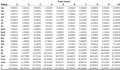
Figure 3.2: Moody's idealized EL values by rating category and tenor

We shall then define EL, the time-continuous version of EL function obtained by linearly interpolating EL between two discrete integer dates:

EL : {1,..,21} x [0,T] -*[0,1]

(m, t) i-* (t + 1 - [t])EL(m, [t]) + (t - [t])EL(m, [t] + 1)

Let us now define the reverse mapping function F ^-1 that transforms any percentage loss level and tenor into a rating:

F -1 : [0, 1] x [0, T] -* {1, .., 21}

(x,t) -* min{m E {1,..,21}| EL(m,t) = x}

We finally give the expression of the Moody's Metric function MM: Definition 3. Moody's Metric

?x E [0,1],?t E [0,T],

EL(F ^-1(x, t), t))

ln x - ln (

MM(x, t) := F ^-1(x, t) + ln ( EL(F ^-1(x, t) + 1, t)) - ln ( EL(F^-1(x, t), t))

In other words, the Moody's Metric can be seen as a standardized continuous scale that allows to compare expected loss levels for different tenors. We shall now take a closer look at the notion of risk measure and understand to what extent it makes sense to use the expected loss as a proxy for measuring risk.

Definition 4. Coherent Risk Measure

Let C denote a set of random variables representing all possible risky positions and L E C be a random variable whose range of values represents possible losses from any given risky position. We define the risk measure function p as a mapping from C to R. The risk measure p is coherent if it is:

i) monotonous: ?X, Y ? G, X = Y p(X) = p(Y )

ii) positively homogeneous: ?X ? G, ?h > 0, hX ? G and p(hX) = hp(X)

iii) sub-additive: ?X, Y ? G, X + Y ? G and p(X + Y ) = p(X) + p(Y )

iv) translation invariant: ?X ? G, ?a ? R s.t. X + a ? G, p(X + a) = p(X) + a

Proposition 4.

If G⁺ is a set of non-negative random variables, interpreted as a loss from a risky position, then expected value is a coherent risk measure:

?X ? G⁺, p(X) := E[X]

Proof. Properties (i),(ii), (iii) and (iv) immediately result from the expectation's linearity.

Unlike E[X], the Moody's Metric MM(X, t), where X is a positive random variable that takes its values in [0, 1], is not a coherent risk measure: though it is clearly monotonous and subadditive (because MM(., t) is increasing and concave), it is neither positively homogeneous, nor translation invariant.