Modeling and forecasting inflation in Rwanda (1995-2009)

My dear parents.

uman beings who are the most to me dear:

Nothing in the world could compensate the sacrifices you have made for my
education and for my welfare so I can focus me on my studies. Able to God, the
Almighty provides you with health, prosperity and longevity.

Thank you for your help, your support and your patience. I dedicate this modest work
as a sign of recognition and of admiration.

I would like to express my gratitude and respectful appreciation to everyone who helped me close or far in the achievement of this work, and more particularly to:

Honorable Senator Professor Dr. RWIGAMBA BALINDA, Founder and President of ULK, for his initiative and innovation for the development of education in our country.

We also wish to thank the Rector of ULK Dr. Alphonse NGAGI and Faculty of ULK more specially those of the Faculty of Economics and Management, especially those of the Economics Department for the scientific support we receive from them.

My gratitude will also to CCA Mme Brigitte GAJU, my direct supervisor for the follow-up given to the conduct of this work: I am very grateful have framed me, lead this work and to ensure its development in not gentle your time or your advice. Be ensured, expensive Supervisor, yours and have my deep respect.

To my classmates of the 4^th year in economics at ULK, promotion 2008 / 2009. We spent of pleasant brotherhood, of camaraderie, effort and perseverance, I hope you all will have one long career in economics and a better life both in terms Professional staff. To all those showing me their sympathy and that I consider as friends full.

Besides my project, I really enjoyed my stay at the NBR, appreciated all the people I worked with and spent good moments with them. That's why I also thank Mr. Boniface MUTABAZI manager of middle office and Pascal MUNYANKINDI for all kind of help. Can God bless you and enables you to perform all your projects and your aspirations!

Ferdinand GAKUBA

ons

ADF: Augmented Dickey Fuller AER: Average Exchange rate

ARCH: Autoregressive Conditional Heteroskedasticity

BNR: National bank of Rwanda CCI: Continuous commodity index CIF: Cost, insurance and freight COLA: Cost of Living Allowance COLI: Cost of living index

CPI: Consumer price index

CRB: Commodity research bureau ECI: Employment cost index

ECM: Error correction model

EURO: European Money

GBP: Great Britain Pound

GDP: Gross domestic production IMF: International Monetary Fund LR: Likelihood ratio

MINECOFIN: Ministère de la finance NSSF: National social security fund OLS: Ordinary Least square

PCEPI: Personal consumption expenditure price index

PPI: Producer price index

RBD: Real bill doctrine

RWF: Rwanda franc

ULK: Université Libre de Kigali

ULC : Unit labour cost.

USA: United State of America

VAR: Vector autoregressive

VECM: Vector error correction model
XDR: Exchange data Representation

Table 2: ADF Statistics for Testing for a Unit Root in all Time Series 34

Table 3: Cointegration analysis in the mark-up model 35

Table 4: Results using OLS 36

Table 5: Properties of VAR residuals 37

Table 6: Standardized adjustment coefficients 38

Table 7: Properties of cointegration vector 38

Table 8: Results for long run inflation model 40

Table 9: Heteroskedasticity test 41

Table 10: Ramsey RESET test 42

Table 11: White test 48

Table 12: ARCH test 48

Table 13: Breusch -Godfrey Test 48

Table 14: Ramsey test 2 49

Table 15: Diagnostic test 52

Table 16: Prevision results 59

Figure 1: Evolution of Inflation in Rwanda 25

Figure 2: Evolution of money supply and CPI 26

Figure 3: Evolution of import prices and domestic prices 27

Figure 4: Evolution of Output and inflation 29

Figure 5: CUSUM Test 42

Figure 6: CUSUM squared test 43

Figure 7: CUSUM stability test (Brown, Durbin, Ewans) 49

Figure 8: CUSUM squared stability test 49

Figure 9: Residuals test 52

Figure 10: Cusum test for Engle- Granger ECM 53

Figure 11: Cusum of squared test for Engle- Granger ECM 53

Figure 12: Inflation forecasting criteria 54

Figure 13: Response function of variables on LIPC 57

Appendix 1: Data description

Appendix 2: Data

Appendix 3: Residuals properties

Appendix 4: VECM results

Appendix 5: Variance decomposition

Appendix 6: Recursive coefficient test

Appendix 7: ECM with Hendry results

Appendix 8: ECM with Engle- Granger results

Acknowledgment ⁱⁱList of acronyms and abbreviations ⁱⁱⁱLIST OF TABLE iv

LIST OF FIGURE v

LIST OF APPENDIX v

TABLE OF CONTENTS vii

Abstract 1

GENERAL INTRODUCTION 2

1. Interest and choice of subject. 2

1.1. Choice 2

1.2. Interests 3

2. Scope of the study

3. Problem statement 3

4. ASSUMPTIONS 4

5. RESEARCH PURPOSE 5

6. RESEARCH TECHNIQUES AND METHODS 5

6.1. TECHNICAL 5

6.1.1. TECHNICAL DOCUMENTARY 5

6.1.2. TECHNICAL INTERVIEW 6

6 .2. METHODS 6

6.2.1. ANALYTICAL METHOD 6

6.2.2. COMPARATIVE METHOD 6

6 .2 .3. STATISTICAL METHOD. 6

7. SUBDIVISION OF WORK 7

CHAPTER I LITERATURE REVIEW 8

1.1. Introduction 8

1.1.1 Inflation 8

1.1.2 Modeling inflation 9

1.1.3 Forecasting inflation 9

1.1.4 Measures of inflation 9

1.2. .Theory of inflation 10

1.2.1 Keynesian view 11

13

ons theory 14

1.2.4 Austrian theory 14

1.2.5 The theory of real bills doctrine 15

1.2.6. Anti-classical or backing theory 16

1.3 The tools for controlling the inflation 16

1.3.1. Monetary policy 16

1.3.2 Fixed exchange rates 17

1.3.3 Wage and price controls 17

1.3.4 Cost-of-living allowance 18

1.4 The history of modeling and forecasting inflation process 19

1.4.1 Some critical issues for modelling 22

1.4.2 Overview of forecasting 22

1.4.2.1 Monetary transmission 23

1.4.2.2. Flexible price equilibrium 24

CHAPTER II. INFLATION MODELLING AND CONCEPTUAL FRAMEWORK 25

2.1. Rwanda's inflation experience 25

2.1.1. Foreign factors 27

2.1.2 Domestic factors 28

2.2. Conceptual framework 29

2.2.1. LONG- RUN RELATIONSHIPS 30

2.2.1.1. Mark up 30

2.2.1.2 Money supply determinants 31

2.2.2. Data descriptions 32

2.3. Estimation of inflation models 33

2.3.1. Mark up 33

2.3.1.1 Integration 33

2.3.1.2. Cointegration 34

2.3.2 Excess money supply 37

2.4 THE LONG RUN MODEL OF INFLATION 38

2.4.1 Interpretation of coefficients 41

2.4.2 Classical Tests 41

CHAPTER III FORECAST INFLATION OF RWANDA USING ECM 45

3.1 Introduction 45

inflation 45

45

3.2.1.1 Long run and short run elasticity 46

3.2.1.2 Significativity of error correction model 47

3.2.2 The ECM with Engle - Granger 50

3.2.2.2 The model properties 52

3.3. Forecasting inflation using VECM 55

3.3.1 Why a VECM? 55

3.3.2. Forecasting performance 56

3.3.2.1 The variance decomposition 58

.3.3.2.2 Forecast results 58

General conclusion 59

Discussion 63

References 64

APPENDIX 67

Inflation constitutes one of the major economic problems in emerging market economies that requires monetary authorities to elaborate tools and policies to prevent high volatility in prices and long periods of inflation. Analysis of inflation and its relationship with the important macroeconomic indicators is an arduous task due to data problems (availability, measurement errors, biases, etc.) and complexity of the transition process experienced by the economy of Rwanda. In order to model inflation dynamics we use the general-to-specific approach. The advantage of this approach is its ability to deliver results based on underlying economic theories of inflation, which are also consistent with the properties of the data. A three steps procedure is followed. In the first step, the long-run sectoral analysis of inflation sources is conducted, yielding long-run determinants of inflation (excess money, nominal effective exchange rate, nominal wages expressed as unit labor cost, import prices, oil prices index and the nominal GDP). In the second step, we estimate an equilibrium error correction model first of all by following Hendry procedures, then building ECM by Engle Granger and compare forecasting criteria of inflation deploying among other variables of interest for the long-run solutions derived in the first step. Lastly, equilibrium error correction model obtained will serve for structural model-based inflation forecasting. Forecasting performance of the model will be compared to other models often utilized for forecasting inflation suggests that markup and excess money relationships are very important for explaining the short-run behaviour of inflation, as well as the output, nominal effective exchange rate, oil prices and import prices in Rwanda.

1. Interest and choice of subject

1.1. Choice

The aim of this paper is to construct a quarterly inflation model and forecasts quarterly-year ahead inflation for Rwanda. Inflation is considered to be a major economic problem in transition economies and thus fighting inflation and maintaining stable prices is the main objective of monetary policy makers. The negative consequences of inflation are well known. Inflation can result in a decrease in the purchasing power of the national currency leading to the aggravation of social conditions and living standards. High prices can also lead to uncertainty making domestic and foreign investors reluctant to invest in the economy. Moreover, inflated prices worsen the country's terms of trade by making domestic goods expensive on regional and world markets.

To develop an effective monetary policy, central banks should possess information on the economic situation in the country, the behaviour and interrelationships of major macroeconomic indicators. Such information would enable the central bank to predict future macroeconomic developments and to react in a proper way to shocks the economy is subject to. Thus, studying inflationary processes is an important issue for monetary economists all around the world. However, it is not an easy task, especially in developing countries, where economic processes are highly unstable and volatile. Moreover, the macroeconomic data on developing countries can be unreliable due to many reasons: measurement error, imperfect methods of measuring, etc. Nevertheless, there exist a number of empirical studies on inflation factors in developing countries.

Since inflation is a phenomenon that characterizes almost all economies as it is developed or not, but particularly developing countries including our country is, within this framework that we considered relevant to the topic, hence the rationale for choosing this subject.

At academic level, this work will constitute an important source of data, both theoretical and practical, researchers, students from different faculties, professors, and all the whole community who will look for modelling and forecasting inflation in their research. This topic has the interest to deepen our understanding of inflation models and its prediction in the context of developing economy and make our contribution to science. This topic has the interest to know the relationship of inflation with others macroeconomic variables

2. Scope of the study

Our research as any other scientific work is limited in time, space and in the domain. In time, we focused our analysis on the period from 1995 to 2009 because the period allowed us to search recent data related to our subject.

Regarding the delimitation of space, our study focuses on Rwandan territory. In the field, our study focuses on macroeconomic.

3. Problem statement

Since Rwanda covered its monetary sovereignty the monetary policy followed was with a direct character thus straightforwardly to manage the banking function this means that the development of its activities was to be contained within the limits deemed compatible with the overall trend of discounting the economy to avoid any risk of deviation¹.

This policy has been unchanged until the end of the Eighties years but like almost everywhere in the world, managed finance proved in Rwanda inefficient and its prevalence has violated not only the conditions of financing the economy but also, and especially, the allowance of the financial resources available and hence two major consequences could appear; the absence of optimal allowance of the financial resources available and sometimes even by monetary creation ex nihilo (excess

¹ Ia politique monétaire au Rwanda; une mutation constante pour une efficience accrue, juin, 2003

g 1990 its was the first foreground of structural

chanism started coming into force then replace the procedures of administrative management. The direct control operated before on both sides by the concerned official structures thus had to disappear gradually and free plan of the supply and the demand were to allow the determination of the different price level of the various markets.

The monetary policy of Rwanda was the subject of a deep change with the imminent emergence of new instruments of the monetary policy which had some modification of the structure to even giving a more and more accentuated at indirect character.

Final objective is the price stability (ultime objective) but the achievement of this objective is conditioned by another intermediate objective that constitutes a walking point which is a vital crossing point of the action of central bank initiated in this context. It acts in the case of Rwanda by controlling the evolution of money supply expressed in a broad sense (M2). Achieving the goal also requires an intermediate operational target which in the context of Rwanda is the monetary base by considering the multiplier stable.

Monetary management ensured by the central Bank of Rwanda still faced major obstacles which affecting more the quality of the results obtained because the lack of a management model that can serve as tool for projecting future, this hampers monetary policy and reach on the price volatility persistence which is his ultimate goal.

The aim of this study is to build a model for the money supply and to build a model of inflation which can be used to forecast the future uncertain. This allows as formulating the following assumptions;

H1: «Inflation is everywhere and always a monetary phenomenon» we wonder if this is same case in Rwanda and what are main causes of inflation in Rwanda?

H2: How can we use these variables to forecast future inflation in Rwanda?

4. HYPOTHESIS

A hypothesis is an early response to questions that arose in the problem and must be confirmed to achieve a result.

hypotheses:

d by excess money supply, However there are other factors like, low level of production, high wages, high level of import rising market prices, nominal exchange rates, and macroeconomic instability, etc.

· . In this way presenting a set of four-step-ahead forecasts bounded by estimated confidence bands we can present an outlook that is more informative about the development of the general direction of prices, and one that explicitly recognizes the uncertainty inherent in forecasting inflation with a long lead. Accordingly, we argue that monetary policy is probably best served by drawing on models that summarize different paradigms of the transmission mechanism, or that use different technical approaches to represent the transmission mechanism. Taking such strategy, diversified approach to inform policy judgements is likely to reduce the risk of making serious policy errors.

5. RESEARCH OBJECTIVES

The main objective of our work is to construct the inflation model which could be

used in short -term forecasting inflation in Rwanda.

In our work we pursue the following specific objectives:

· Show the different variables which explain inflation in Rwanda

· Propose economic policies to fight against inflation in Rwanda

· Give the model of inflation which should be used as forecast tool

6. RESEARCH TECHNIQUES AND METHODS

6.1. TECHNIQUES of inflation deploying, among other variables of interest

A technique is defined as all resources and processes that enable researchers to gather data and information on the research topic².

Thus, we preferred the following techniques:

6.1.1. DOCUMENTARY TECHNIQUE

² WELMAN J. C and KRUGER S.J.(2001) : Research methodology course for the business and administrative sceines , 2^nd edition , Paris, Durod , page 34

s a systematic search of all that is written related with the research area such as books, pamphlets, monographs, unpublished documents, reports, budgets, public records etc. the documentary technical allows us to choice among the books available what are useful for our research and help to use the best resources.

6.1.2. TECHNIQUE OF INTERVIEW

This technique is to maintain discussions and dialogues with people who provide the researcher's information on his research topic. This technique allowed us to interact with senior officials of the Rwanda Revenue Authority, those of MINECOFIN and BNR those of us who have talked about everything that is related to inflation in Rwanda.

6 .2. METHODS

A method is defined as an ordered set of rules and principles of intellectual operations to do the analysis to achieve a result³.

At the completion of our work, we have chosen the following methods:

6.2.1. ANALYTICAL METHOD

This method allows to systematically analyzing all information and data collected. It allowed us to systematically analyze the inflation's relationship with others macroeconomic variables, to interpret and draw the conclusion.

6.2.2. COMPARATIVE METHOD

This method allowed us to compare model adopted with others to identify the link between those.

6 .2 .3. STATISTICAL METHOD

³ WELMAN J. C and KRUGER S.J.(2001) : Research methodology course for the business and administrative sceines , 2^nd edition , Paris, Durod , page 36

ing the data, synthesizing the results of research by first. Second, it allowed us to present these results as graphs, tables, to facilitate reading and understanding of our work.

7. ORGANIZATIONAL OF WORK

Besides the general introduction, this work is organised as follows. In chapter one we will state some empirical literature. Chapter 2 illustrates the identification of the inflation models. Chapter 3 gives the description of Error correction models, forecasting principles and the estimation results. In that version of the VECM, some variables are exogenous or became unstable in simulations over the long run. In the extended version of the VECM developed here, we impose sensible long-run conditions that help to determine the behaviour of the inflation for Rwanda, interest rates, and the exchange rate. As result, we should be able to have more confidence in the long-run and dynamic properties of the model.

The third chapter deals with the analysis of inflation; we consider the forecast accuracy of the extended VECM in an unconditional, out-of-sample exercise. We also illustrate that a more informative way to present inflation forecasts than simply providing the point estimate of the model is to include as well a statement about the probability distribution of potential outcomes. By drawing on the model's estimated variance covariance matrix, we generate confidence intervals around a set of 4-stepahead forecasts, with each forecast projecting the one quarter inflation rate six-quarter further into the future.

Finally, we will close our work with a general conclusion and discussion.

EW

1.1.Introduction

1.1.1 Inflation

In economics, inflation is a rise in the general level of prices of goods and services in an economy over a period of time⁴. When the price level rises, each unit of currency buys fewer goods and services; consequently, inflation is also erosion in the purchasing power of money a loss of real value in the internal medium of exchange and unit of account in the economy⁵. A chief measure of price inflation is the inflation rate, the annualized percentage change in a general price index (normally the consumer price index over time).

The term "inflation" usually refers to a measured rise in a broad price index that represents the overall level of prices in goods and services in the economy. The Consumer Price Index (CPI), the Personal Consumption Expenditures Price Index (PCEPI) and the GDP deflator are some examples of broad price indices⁶. The term inflation may also be used to describe the rising level of prices in a narrow set of assets, goods or services within the economy, such as commodities (which include food, fuel, metals), financial assets (such as stocks, bonds and real estate), and services (such as entertainment and health care). The Reuters-CRB Index (CCI), the Producer Price Index, and Employment Cost Index (ECI) are examples of narrow price indices used to measure price inflation in particular sectors of the economy. Asset price inflation is a rise in the price of assets, as opposed to goods and services⁷. Core inflation is a measure of price fluctuations in a sub-set of the broad price index which excludes food and energy prices⁸. The Federal Reserve Board uses the core inflation rate to measure overall inflation, eliminating food and energy

⁴ Abel & Bernanke (1995); Inflation determinants in transition economy, November ,2006

⁵ Walgenbach P. H., Norman E. Dittrich and Ernest I. Hanson, (1973), The Measuring Unit principle, Page 429

⁶ Blundell-Wignall, A.(ed.)(1992), Inflation, Disinflation and Monetary Policy, Reserve Bank of Australia, Sydney, page 112

⁷ http://en.wikipedia.org/wiki/Asset_price_inflation

⁸ Robert Rich, Charles Steindel (2005):A Review of Core Inflation and an Evaluation of Its Measures (Staff Report, Federal Reserve Bank of New York

rm price fluctuations that could distort estimates of the general economy^9.

1.1.2 Modeling inflation

Modeling inflation is a simplified representation of inflation system or phenomenon, as in the sciences or economics, with any hypotheses required to describe the system or explain the phenomenon, often mathematically¹⁰.

1.1.3 Forecasting inflation

The forecasting inflation is one of the tools which can be used with the policy makers when the policy adopted by central bank has inflation as ultime objective for monetary purpose it helps by explaining its uses and how it relates to planning and formulate the problem to the use of the forecast¹¹.

1.1.4 Measures of inflation

Inflation is usually estimated by calculating the inflation rate of a price index, usually the Consumer Price Index. The Consumer Price Index measures prices of a selection of goods and services purchased by a "typical consumer" The inflation rate is the percentage rate of change of a price index over time¹²

Other widely used price indices for calculating price inflation include the following:

· Cost-of-living index (COLI) is index similar to the CPI which is often used to adjust fixed incomes and contractual incomes to maintain the real value of those incomes.

· Producer price index (PPI) which measures average changes in prices received by domestic producers for their output¹³. This differs from the CPI in that price subsidization, profits, and taxes may cause the amount received by

⁹ Kiley, Michael J. (2008). Estimating the common trend rate of inflation for consumer prices and consumer prices excluding food and energy prices, Federal Reserve Board

10 Encyclopedia

¹¹ Armstrong J. S (2001):Principles of forecasting; A handbook for researchers and practitioners, USA 2001

¹² Taylor & Hall 1993

¹³ Encyclopedia

what the consumer paid. There is also typically a

e in the PPI and any eventual increase in the CPI. Producer price index measures the pressure being put on producers by the costs of their raw materials. This could be "passed on" to consumers, or it could be absorbed by profits, or offset by increasing productivity.

· Commodity price indices, which measure the price of a selection of commodities. In the present commodity price indices are weighted by the relative importance of the components to the "all in" cost of an employee.

· Core price indices: because food and oil prices can change quickly due to changes in supply and demand conditions in the food and oil markets, it can be difficult to detect the long run trend in price levels when those prices are included.

Other common measures of inflation are:

· GDP deflator is a measure of the price of all the goods and services included Gross Domestic Product (GDP). The Rwanda Commerce Department publishes a deflator series for Rwanda GDP, defined as its nominal GDP measure divided by its real GDP measure.

Asset price inflation is an undue increase in the prices of real or financial assets, such as stock (equity) and real estate. While there is no widely-accepted index of this type, some central bankers have suggested that it would be better to aim at stabilizing a wider general price level inflation measure that includes some asset prices, instead of stabilizing CPI or core inflation only. The reason is that by raising interest rates when stock prices or real estate prices rise, and lowering them when these asset prices fall, central banks might be more successful in avoiding bubbles and crashes in asset prices¹⁴.

1.2..Theory of inflation

Historically, a great deal of economic literature was concerned with the question of
what causes inflation and what effect it has. There were different schools of thought
as to the causes of inflation. Most can be divided into two broad areas: quality

theories of inflation. The quality theory of inflation

ler accepting currency to be able to exchange that currency at a later time for goods that are desirable as a buyer. The quantity theory of inflation rests on the quantity equation of money, that relates the money supply, its velocity, and the nominal value of exchanges. Adam Smith and David Hume proposed a quantity theory of inflation for money, and a quality theory of inflation for production.

Currently, the quantity theory of money is widely accepted as an accurate model of inflation in the long run. Consequently, there is now broad agreement among economists that in the long run, the inflation rate is essentially dependent on the growth rate of money supply. However, in the short and medium term inflation may be affected by supply and demand pressures in the economy, and influenced by the relative elasticity of wages, prices and interest rates¹⁵.

The question of whether the short-term effects last long enough to be important is the central topic of debate between monetarist and Keynesian economists. In monetarism prices and wages adjust quickly enough to make other factors merely marginal behavior on a general trend-line. In the Keynesian view, prices and wages adjust at different rates, and these differences have enough effects on real output to be "long term" in the view of people in an economy.

1.2.1 Keynesian view

Keynesian economic theory proposes that changes in money supply do not directly affect prices, and that visible inflation is the result of pressures in the economy expressing themselves in prices. The supply of money is a major, but not the only, cause of inflation. There are three major types of inflation, as part of what Robert J. Gordon calls the "triangle model¹⁶":

¹⁴ Mankiw (2002): Macroeconomics principles,, p. 22-32

15 Federal Reserve Board's semiannual Monetary Policy Report to the Congress Round table; Introductory statement by Jean-Claude Trichet on July 1, 2004

¹⁶ Robert J. Gordon (1988), Macroeconomics, Addison Wesley, 2002 ISBN 0-201-77036-9

caused by increases in aggregate demand due to

overnment spending, etc¹⁷. Demand inflation is constructive to a faster rate of economic growth since the excess demand and favorable market conditions will stimulate investment and expansion.

· Cost-push inflation, also called "supply shock inflation," is caused by a drop in aggregate supply (potential output). This may be due to natural disasters, or increased prices of inputs. For example, a sudden decrease in the supply of oil, leading to increased oil prices, can cause cost-push inflation. Producers for whom oil is a part of their costs could then pass this on to consumers in the form of increased prices¹⁸.

· Built-in inflation or structural inflation is an economic term referring to type of inflation that result from past events and persists in the present. It thus might be called hangover inflation, expectations, and is often linked to the "price/wage spiral". It involves workers trying to keep their wages up with prices (above the rate of inflation), and firms passing these higher labor costs on to their customers as higher prices, leading to a 'vicious circle'. Built-in inflation reflects events in the past, and so might be seen as hang over inflation¹⁹.

Some Keynesian economists also disagree with the notion that central banks fully control the money supply, arguing that central banks have little control, since the money supply adapts to the demand for bank credit issued by commercial banks²⁰. This is known as the theory of endogenous money, and has been advocated strongly by post-Keynesians as far back as the 1960s. It has today become a central focus of Taylor rule advocates. This position is not universally accepted banks create money by making loans, but the aggregate volume of these loans diminishes as real interest rates increase. Thus, central banks can influence the money supply by making money cheaper or more expensive, thus increasing or decreasing its production.

A fundamental concept in inflation analysis is the relationship between inflation and unemployment, called the Phillips curve. This model suggests that there is a trade-off

17 http://www.bized.co.uk/virtual/bank/economics/mpol/inflation/causes/theories1.htm,Retrieved 1/11/2009

¹⁸ Encyclopedia Britannica, "The cost-push theory"

¹⁹ http://en.wikipedia.org/wiki/Built-in_inflation, Retrieved 1/11/2009

oyment. Therefore, some level of inflation could be

minimize unemployment. The Phillips curve model described the U.S. experience well in the 1960s but failed to describe the combination of rising inflation and economic stagnation (sometimes referred to as stagflation) experienced in the 1970s²¹

1.2.2 Monetarist view

Monetarists believe the most significant factor influencing inflation or deflation is the management of money supply through the easing or tightening of credit. They consider fiscal policy, or government spending and taxation, as ineffective in controlling inflation²².

Monetarists assert that the empirical study of monetary history shows that inflation has always been a monetary phenomenon. The quantity theory of money, simply stated, says that the total amount of spending in an economy is primarily determined by the total amount of money in existence. This theory begins with the identity:

Where;

M is the quantity of money.

V is the velocity of money in final expenditures;

P is the general price level;

Q is an index of the real value of final expenditures;

In this formula, the general price level is affected by the level of economic activity (Q), the quantity of money (M) and the velocity of money (V). The formula is an identity because the velocity of money (V) is defined to be the ratio of final expenditure to the quantity of money (M).

Velocity of money is often assumed to be constant, and the real value of output is
determined in the long run by the productive capacity of the economy. Under these

²⁰ Gordon, Robert J. (2000), "Does the 'New Economy' measure up to the great Inventions of the Past?", Journal of Economic Perspectives 14 (4): 49-74

²¹ Mankiw 2002,Macroeconomics principles, p. 65-77

f the change in the general price level is changes in

nstant velocity, the money supply determines the value of nominal output (which equals final expenditure) in the short run. In practice, velocity is not constant, and can only be measured indirectly and so the formula does not necessarily imply a stable relationship between money supply and nominal output. However, in the long run, changes in money supply and level of economic activity usually dwarf changes in velocity. If velocity is relatively constant, the long run rate of increase in prices (inflation) is equal to the difference between the long run growth rate of money supply and the long run growth rate of real output²³.

1.2.3. Rational expectations theory

Rational expectations theory holds that economic actors look rationally into the future when trying to maximize their well-being, and do not respond solely to immediate opportunity costs and pressures²⁴. In this view, while generally grounded in monetarism, future expectations and strategies are important for inflation as well.

A core assertion of rational expectations theory is that actors will seek to "head off" central-bank decisions by acting in ways that fulfill predictions of higher inflation. This means that central banks must establish their credibility in fighting inflation, or have economic actors²⁵ make bets that the economy will expand, believing that the central bank will expand the money supply rather than allow a recession.

1.2.4 Austrian theory

The Austrian School asserts that inflation is an increase in the money supply, rising prices are merely consequences and this semantic difference is important in defining inflation²⁶

Austrian economists believe that there is no material difference between the
concepts of monetary inflation and general price inflation. Austrian economists

²² Lagassé, Paul (2000).Columbia encyclpedia,ISBN-10 0787650153 page 556-558

²³ Mankiw 2002, Macroeconomics principles, pp. 81-107

24 Dowyer,J.and R. Lam (1994), Economic and Financial Research in the Reserve Bank in 1994

25 Sargent, Thomas J. Rational Expectations and Inflation. New York: Harper and Row, 1986.

²⁶ Shostak, Ph. D, Frank (2002-03-02). "Defining Inflation". Mises Institute. http://mises.org/story/908. Retrieved 2009-10-10

lculating the growth of new units of money that are change, that have been created over time²⁷.

This interpretation of inflation implies that inflation is always a distinct action taken by the central government or its central bank, which permits or allows an increase in the money supply²⁸. In addition to state-induced monetary expansion, the Austrian School also maintains that the effects of increasing the money supply are magnified by credit expansion, as a result of the fractional-reserve banking system employed in most economic and financial systems in the world²⁹

Austrians argue that the state uses inflation as one of the three means by which it can fund its activities (inflation tax), the other two being taxation and borrowing. Various forms of military spending is often cited as a reason for resorting to inflation and borrowing, as this can be a short term way of acquiring marketable resources and is often favored by desperate, indebted governments³⁰.

1.2.5 The theory of real bills doctrine

Within the context of a fixed species basis for money, one important controversy was between the quantity theory of money and the real bills doctrine (RBD). Within this context, quantity theory applies to the level of fractional reserve accounting allowed against specie, generally gold, held by a bank. Currency and banking schools of economics argue the RBD, that banks should also be able to issue currency against bills of trading, which is "real bills" that they buy from merchants. This theory was important in the 19th century in debates between "Banking" and "Currency" schools of monetary soundness, and in the formation of the Federal Reserve. In the wake of the collapse of the international gold standard post 1913, and the move towards deficit financing of government, RBD has remained a minor topic, primarily of interest in limited contexts, such as currency boards. It is generally held in ill repute today, with Frederic Mishkin, a governor of the Federal Reserve going so far as to say it had been "completely discredited." Even so, it has theoretical support from a few

²⁷ Joseph T. Salerno, (1987), Austrian Economic Newsletter, "<a href=" http://www.mises.org/journals/aen Retrieved 2009-10-10

²⁸ Ludwig von Mises Institute, "True Money Supply; page 456

²⁹ Joseph T. Salerno, (1987),Quarterly Journal of economics Facts, Discussion Forum -356

at see restrictions on a particular class of credit as nciples of laissez-faire, even though almost all libertarian economists are opposed to the RBD.

The debate between currency, or quantity theory, and banking schools in Britain during the 19th century prefigures current questions about the credibility of money in the present. In the 19th century the banking school had greater influence in policy in the United States and Great Britain, while the currency school had more influence "on the continent", that is in non-British countries, particularly in the Latin Monetary Union and the earlier Scandinavia monetary union³¹.

1.2.6. Anti-classical or backing theory

Another issue associated with classical political economy is the anti-classical hypothesis of money, or "backing theory". The backing theory argues that the value of money is determined by the assets and liabilities of the issuing agency³². Unlike the Quantity Theory of classical political economy, the backing theory argues that issuing authorities can issue money without causing inflation so long as the money issuer has sufficient assets to cover redemptions.

1.3 The tools for controlling the inflation

A variety of methods have been used in attempts to control inflation.

1.3.1. Monetary policy

Monetarists emphasize keeping the growth rate of money steady, and using monetary policy to control inflation (increasing interest rates, slowing the rise in the money supply). Keynesians emphasize reducing aggregate demand during economic expansions and increasing demand during recessions to keep inflation stable. Control of aggregate demand can be achieved using both monetary policy and fiscal policy (increased taxation or reduced government spending to reduce

³⁰ Ludwig von Mises, The Theory of Money and Credit, page23-56

³¹ Selgin, G. A, "The Analytical Framework of the Real Bills Doctrine",Journal of Institutional and Theoretical Economics, volume 145, (1989), p. 489.

³² Ron Paul, "The Case for Gold, page 45-56

l for controlling inflation is monetary policy. Most ping the federal funds lending rate at a low level.

1.3.2 Fixed exchange rates

Under a fixed exchange rate currency regime, a country's currency is tied in value to another single currency or to a basket of other currencies (or sometimes to another measure of value, such as gold). A fixed exchange rate is usually used to stabilize the value of a currency, vis-à-vis the currency it is pegged to. It can also be used as a means to control inflation. However, as the value of the reference currency rises and falls, so does the currency pegged to it. This essentially means that the inflation rate in the fixed exchange rate country is determined by the inflation rate of the country the currency is pegged to. In addition, a fixed exchange rate prevents a government from using domestic monetary policy in order to achieve macroeconomic stability.

Under the Bretton Woods agreement, most countries around the world had currencies that were fixed to the US dollar. This limited inflation in those countries, but also exposed them to the danger of speculative attacks. After the Bretton Woods agreement broke down in the early 1970s, countries gradually turned to floating exchange rates. However, in the later part of the 20th century, some countries reverted to a fixed exchange rate as part of an attempt to control inflation. This policy of using a fixed exchange rate to control inflation was used in many countries in South America in the later part of the 20th century (e.g. Argentina (1991-2002), Bolivia, Brazil, and Chile)³³.

1.3.3 Wage and price controls

Another method attempted in the past has been wage and price controls ("incomes policies"). Wage and price controls have been successful in wartime environments in combination with rationing. However, their use in other contexts is far more mixed. Notable failures of their use include the 1972 imposition of wage and price controls

³³ Edwards, Sebastian. (2002) The Great Exchange Rate Debate after Argentina, The North American Journal of Economics and Finance, Volume 13, Issue 3, pp. 237-252

essful examples include the Prices and Incomes enaar Agreement in the Netherlands.

In general wage and price controls are regarded as a temporary and exceptional measure, only effective when coupled with policies designed to reduce the underlying causes of inflation during the wage and price control regime, for example, winning the war being fought. They often have perverse effects, due to the distorted signals they send to the market. Artificially low prices often cause rationing and shortages and discourage future investment, resulting in yet further shortages. The usual economic analysis is that any product or service that is under-priced is over consumed.

However, in general the advice of economists is not to impose price controls but to liberalize prices by assuming that the economy will adjust and abandon unprofitable economic activity. The lower activity will place fewer demands on whatever commodities were driving inflation, whether labor or resources, and inflation will fall with total economic output. This often produces a severe recession, as productive capacity is reallocated and is thus often very unpopular with the people whose livelihoods are destroyed.

1.3.4 Cost-of-living allowance

The real purchasing-power of fixed payments is eroded by inflation unless they are inflation-adjusted to keep their real values constant. In many countries, employment contracts, pension benefits, and government entitlements (such as social security) are tied to a cost-of-living index, typically to the consumer price index³⁵. A cost-ofliving allowance (COLA) adjusts salaries based on changes in a cost-of-living index. Salaries are typically adjusted annually. They may also be tied to a cost-of-living index that varies by geographic location if the employee moves.

Annual escalation clauses in employment contracts can specify retroactive or future
percentage increases in worker pay which are not tied to any index. These

³⁴Richard Milhous Nixon (January 9, 1913 - April 22, 1994) was the 37th President of the United States (1969- 1974) and is the only president to resign the office. He was also the 36th Vice President of the United States (1953-1961). See bibliography USA president

colloquially referred to as cost-of-living adjustments

se of their similarity to increases tied to externally-determined indexes. Many economists and compensation analysts consider the idea of predetermined future "cost of living increases" to be misleading for two reasons:

(1) For most recent periods in the industrialized world, average wages have increased faster than most calculated cost-of-living indexes, reflecting the influence of rising productivity and worker bargaining power rather than simply living costs, and

(2) Most cost-of-living indexes are not forward-looking, but instead compare current or historical data.

1.4 The history of modeling and forecasting inflation process

Since inflation was an economic issue numerous attempt to model inflation in developed countries as well as developing countries was made. For example, Juselius (1992) in her seminal paper on inflation modeling in a small open economy studied the inflationary processes in Denmark. De Brower and Ericsson (1998) wrote an appealing paper on inflation modeling in Australia.

Both studies serve as important theoretical and methodological references for our later empirical research in the field of macroeconomic modeling. Welfe (2000) modeled inflation in Poland, accounting for a number of important features that characterize a transition economy. Besides these, worth noting are Ramakrishnan and Vamvakidis (2002)who worked on a model to forecast inflation behavior in Indonesia, and Callen and Chang (1999) who conducted an empirical study on inflation in India.

Most of the literature in the field constitutes empirical studies for modeling inflationary processes in different countries and inflation factors in general. These studies follow approaches based on different economic theories, choosing the most appropriate for the economy investigated.

³⁵ DeLong, Brad. «Why Not the Gold Standard?» http://www.j-bradford-
delong.net/Politics/whynotthegoldstandard.html. Retrieved 2009-09-25.

nflation, the study by Loungani and Swagel (2001)

s a starting point for understanding inflation in developing countries. The authors present stylized facts about inflation behavior in developing countries, focusing primarily on the relationship between the exchange rate regime and the sources of inflation. Another important study of inflationary processes was accomplished by Fischer, Sahay, and Végh (2002) on the experiences of hyper and high inflations in various countries. The authors found that there is a very strong relationship between money growth and inflation both in the long and short run.

Golinelli and Orsi (2002) study the inflation processes in three new EU member countries: the Czech Republic, Hungary and Poland. All three countries possess a similar historico- conomic background and similar economic context: they were administrative economies before and have undergone major systemic changes during the transition to a market economy. Investigating inflationary processes in these countries is of great importance because all countries experienced high inflation episodes during the years of transition, and price stabilization policies played an important role in their successful transition to a new economic system. The authors follow a methodology very close to that of Juselius (1992) in modeling inflation behavior in the countries under consideration. They use the multivariate VAR approach, grouping together those determinants that belong to main inflation theories: cost pushed inflation, foreign prices and exchange rates, and excess money. Further, a vector equilibrium correction model specification is used since it enables capturing short-term dynamics by including stationary variables and past imbalances, i.e.the «gaps» detected by previous cointegrated relationships.

In his study on the determinants of inflation in Ukraine, the author, Lissovolik (2003), studies the factors of inflation in Ukraine during the period from 1993 to 2002, the so-called «transition period». The most relevant stylized facts important for modeling inflation behavior in Ukraine appear to be domestic financial instability, external disequilibria, seasonality of the economy, and allowance for an increase in administered prices. The resulting equation of an inflation model is a version of a long-term markup of prices over wages, the exchange rate, administrative prices, short-term factors and dummy variables.

are concerned with the problem of significant dollarization in transition economies, and its impact on the money demand and inflation. In particular, the authors study the case of Russia, and illustrate that all the measures of money aggregates that exclude foreign currency are negatively correlated with the nominal depreciation rate. This could suggest that foreign currency has been an important substitute for domestic money. The authors estimate an equilibrium correction model (ECM) for inflation in order to identify how the short-term dynamics of inflation are affected by deviations from the long-term money demand equation. They found that inflation does not react significantly to the excess supply of monetary aggregates that exclude foreign currency. Payne (2002) explores inflationary dynamics in Croatia using vector auto regression over the period January 1992-December 1999. The VAR incorporated four variables: broad money supply, retail price index1, nominal net wage per employee and the nominal effective exchange rate³⁶. The model results suggest that wage increase and currency depreciation are positively correlated with inflation rates.

Building on Paynes model, BotriL and Cota (2006) model Croatian inflation dynamics using structural vector autoregression³⁷. Thay found that terms of trade and balance of payment shocks have the strongest impact on prices. The authors find justification for such result in Croatia being a small open economy with high import dependency and uncompetitive economic structure. In order to contrast these findings, the authors also re-estimated Paynes model. While Paynes conclusion on influence of wages and currency depreciation on prices still holds, in newly estimated four-variable VAR positive correlation between broad money and prices and some inflation inertia also emerged.

36 Payne, James E., 2002, «Inflationary Dynamics of a Transition Economy: the Croatian

Experience», Journal of Policy Modeling, 24(3), pp. 219-30.

37 Botri[I, Valerija and Boris Cota, 2006, «Sources of Inflation in Transition Economy: The Case of Croatia», Ekonomski pregled, 57(12), pp. 835-855.

odelling

The quantitative macroeconomic modelling fell out of favour during the 1970s for two related reasons: First, some of the existing models, like the Wharton econometric model and the Brookings model, failed spectacularly to forecast the stagflation of the 1970s. Second, leading macroeconomists levelled harsh criticisms of these frameworks. Lucas (1976) and Sargent (1981), for example, argued that the absence of an optimization-based approach to the development of the structural equations meant that the estimated model coefficients were likely not invariant to shifts in policy regimes or other types of structural changes. Similarly, Sims (1980) argued that the absence of convincing identifying assumptions to sort out the vast simultaneity among macroeconomic variables meant that one could have little confidence that the parameter estimates would be stable across different regimes. These powerful critiques clarified why econometric models fit largely on statistical relationships from a previous era did not survive the structural changes of the 1970s.

1.4.2 Overview of forecasting

Forecasting inflation is clearly of critical importance to the conduct of monetary policy, regardless of whether or not the central bank has a numerical inflation target.There are many literatures about inflation forecast for example using the generalized Phillips curves (i.e. using forecasting models where inflation depends on past inflation, the unemployment rate and other predictors) developed by Dimitris K.(2009)³⁸ This literature is too voluminous to survey here, but a few representative and influential papers include Ang, Bekaert and Wei (2007), Atkeson and Ohanian (2001), Groen, Paap and Ravazzolo (2008) and Stock and Watson (1999). The details of these papers differ, but the general framework involves a dependent variable such as inflation (or the change in inflation) and explanatory variables including lags of inflation, the unemployment rate and other predictors. Recursive,regression-based methods, have had some success. However, three issues arise when using such methods.

³⁸Gary K. and Dimitris K.(2009); Forecasting Inflation Using Dynamic Model Averaging, University of Strathclyde, June 2009

edictors can change over time. For instance, it is commonly thought that the slope of the Phillips curve has changed over time. If so, the coefficients on the predictors that determine this slope will be changing (Stock and Watson, 1996).

Second, the number of potential predictors can be large. For instance, Groen, Paap and Ravazzolo (2008) consider ten predictors. Researchers working with factor models such as Stock and Watson (1999) typically have many more than this. The existence of so many predictors can result in a huge number of models.

Third, the model relevant for forecasting can potentially change over time. For instance, the set of predictors for inflation may have been different in the 1970s than now or some variables may predict well in recessions but not in expansions. This kind of issue further complicates an already difficult econometric exercise³⁹.

Among other things, we describe the key differences with respect to the earlier generation of macro models. In doing so, we highlight the insights for policy that these new frameworks have to offer. In particular, we will emphasize two key implications of these new frameworks.

1.4.2.1 Monetary transmission

Monetary transmission depends critically on private sector expectations of the future path of the central bank's policy instrument, the short-term interest rate. Ever since the rational expectations revolution, it has been well understood that the effects of monetary policy depend on private sector expectations. This early literature, however, typically studied how expectations formation influenced the effect of a contemporaneous shift in the money supply on real versus nominal variables (for example, Fischer, 1977; Taylor, 1980).

In this regard, the new literature differs in two important ways. First, as we discuss
below, it recognizes that central banks typically employ a short-term interest rate as
the policy instrument. Second, within the model, expectations of the future

39 Stock, J. and Watson M., 1999. Forecasting inflation: Journal of Monetary Economics 44, 293-335.

er the structural equations, since these aggregate

king decisions by individual households and firms. As a consequence, the current values of aggregate output and inflation depend not only on the central bank's current choice of the short-term interest rate, but also on the anticipated future path of this instrument. The practical implication is that how well the central bank is able to manage private sector expectations about its future policy settings has important consequences for its overall effectiveness. Put differently, in these paradigms the policy process is as much, if not more, about communicating the future intentions of policy in a transparent way, as it is about choosing the current policy instrument. In this respect, these models provide a clear rationale for the movement toward greater transparency in intentions that central banks around the globe appear to be pursuing.

1.4.2.2. Flexible price equilibrium

The natural (flexible price equilibrium) values of both output and the real interest rate provide important reference points for monetary policy and may fluctuate considerably. While nominal rigidities are introduced in these new models in a more rigorous manner than was done previously, it remains true that one can define natural values for output and the real interest rate that would arise in equilibrium if these frictions were absent. These natural values provide important benchmarks, in part because they reflect the (constrained) efficient level of economic activity and also in part because monetary policy cannot create persistent departures from the natural values without inducing either inflationary or deflationary pressures. Within traditional frameworks, the natural levels of output and the real interest rate are typically modeled as smoothed trends. Within the new frameworks they are modelled explicitly.

This book has two broad goals. The first goal is to present econometric evidence on which type of monetary policy rule is likely to be both efficient and robust when used as a guideline for the conduct of monetary policy in Rwanda. The second goal is to answer several current monetary policy questions such as the effects of uncertainty about potential GDP growth or the role of the inflation rate in the setting of interest rates that are most naturally addressed within a framework of monetary policy rules.

ELLING AND CONCEPTUAL FRAMEWORK

A main objective of this chapter is to find the relevant long- run relationships of inflation and economics variables which driver the Rwanda inflation and to examine whether we can come up with a reasonable inflation function by imposing these relationships as equilibrium corrections terms. This chapter will help to answer the first of assumption which state as; inflation is in Rwanda a monetary phenomenon? And what are the drivers it in Rwanda?

2.1. Rwanda's inflation experience

Inflation in Rwanda over the past fifteen years has been mainly influenced by the excess money supply and the nature of import arrangement and the country's openness. Over these fifteen years ago the evolution of inflation has been notably similar to that in developed countries and some in developing countries in the region.

Figure 1: Evolution of Inflation in Rwanda

IPC

2.0 1.8 1.6 1.4 1.2 1.0 0.8 0.6
	1996 1998 2000 2002 2004 2006 2008

Source: Author plotting (see appendix 2)

On the right side (axis) there evolution in year starting by 1995 until 2009 and on the left hand (absisse) are rate of increase by quarterly basis as we see on the figure 1 since the 1995 the inflation rise with a constant rate of 0.3% but during 2006 the rate change 0.6% which is high movement of change until 2009 this was due to first of all the increase in salaries in 2006 and 2008 the oil shocks.

in Rwanda started to rise in the middle of 2007 8 as result of the oils price shocks. However the

rise observed in mid 1998 was due to genocide event which hit all economics sector and kill around one million of Rwandan people and demonetization process which took place during that period.

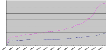
Figure 2: Evolution of money supply and CPI

700.00

600.00

500.00

400.00

300.00

200.00

100.00

0.00

ipc M2

Source: Author plotting (data see appendix 2)

On the right hand the evolution in year and on the left hand the increase of money supply. From 1995 the money supply was tie to economic activities and as the money supply increased, the inflation follow the speed of money supply until 2001 but after this period the CPI slope (red on up) become more positive compare to slope of money supply this mean that there other factor which come into force to explain the increase of price level among those for example is the decrease of national output and lack of food in many area such as Bugesera, and others.

The close correspondence between domestic and foreign inflation points to the importance of foreign factors (the role of import arrangement) in underpinning Rwanda major inflationary episodes.

y and a variety of theoretical models give the result that for a small country; foreign inflation will be fully imported in the long run under a regime of fixed exchange rate. In effect, a small country with a fixed exchange rate has very little choice but to accommodate foreign shocks to price. Although since the Central bank hasn't this regime in Rwanda its use a range of tools which may ameliorate the effects of foreign price shocks the picture in Rwanda as in most other developing countries with similar institutions structures is of the shocks originating in the balance of payments and impacting through the exchange mechanism. With well over half of Rwanda goods and services imported there remains a close correspondence between foreign and domestic prices (see Figure 3).

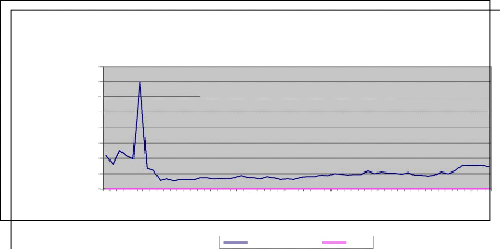
Figure 3: Evolution of import prices and domestic prices

T

o

some in thousand

4000000

2500000

2000000

3500000

3000000

1500000

1000000

500000

1995-1 1996-1 1997-1 1998-1 1999-1 2000-1 2001-1 2002-1 2003-1 2004-1 2005-1 2006-1 2007-1 2008-1 2009-1

0

I lower the

import price IPC

period in years

port price

price. Since 1995 until 1996 the quantity imported was very high and import price also was very big but at the same time the domestic price was not very high because at this period the most commodities imported was not for consumption. There were dominated by services and low materials to build and medical stuffs. After the 1998 the situation change first of all by lack of food because there was insecurity in whole country this impel people to cultivate and making there daily activities the high level of price was due of food products. Since the 2002 the speed in import price was is

e level on domestic market.

2.1.2 Domestic factors

Its have been seen foreign factors have played a dominant role, domestic factors also appear to have underpinned inflation over much of the period and have been particularly important during the keys period. The nominal wage grew at an average annual rate of over six percent over the past fifteen years while productivity grew on average of two percent. The result was sustained growth in nominal unit labor cost which effectively put a floor under domestic inflation( see Figure4) sharp increase in real wages particularly during the 2006 appear to have intensified price pressure at the time.

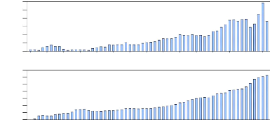
Figure4: Evolution of nominal wage and CPI

UUC

96 98 00 02 04 06 08

.018

.016

.014

.012

.010

.008

.006

2.0

0.8

0.6

1.8

1.6

1.4

1.2

1.0

96 98 00 02 04 06 08

IPC

Source: Author plotting (data appendix1)

One the right hand is the evolution in year and left hand the rate of change in nominal wage and the consumer price index for domestic goods. While broad movements in prices appear to have been largely caused by import prices and domestic labour costs, there also appears to have been a correlation with the cyclical pattern of output. Domestic business cycle fluctuations often reflect a misalignment of demand and the productive capacity of the economy. Excess demand is likely to generate price pressures in factor and product markets (see Figure 5)

nflation

IIC

2.0

1.8

1.6

1.4

1.2

1.0

0.8

0.6

96 98 00 02 04 06 08

IIBC

6E-.-12 5E-.-12 4E-.-12 3E-.-12 2E-.-12 1E-.-12 0E-.-00
	96 98 00 02 04 06 08

Source: Author plotting (data appendix1) 1

The figure above show the correlation between the increase in out put on the right hand the two year evolution and the left hand the rate of price level increased the expectation here is that the increase of price was not due to increase of output but the output seems to be positive by the way the level of domestic demand was not compensated by domestic production this explain the need of import which was observed above.

Macroeconomic theory suggests different way to explain the problem of inflation. The basic concept to be considered is the models suggested by Brouwer and Neil R.Ericsson which reconciles the effects of «demand-pull» and «cost -push» inflation theory.

2.2. Conceptual framework

Inflation is thought to be an outcome of various economic factors. In Rwanda context we choice the factors from supply side that come from cost-push or mark up relationships; the demand side factors that may cause the demand pull inflation; monetary factors ; and foreign factors like exchange rate effects. In order to capture the various determinants of inflation we will combine the methodology developed in Brouwer and Neil R. Ericsson (1998) and Juselius(1992). The mark up model has a

resence in economics generally; see Duesenberry 93).

2.2.1. LONG- RUN RELATIONSHIPS 2.2.1.1. Mark up

We Investigate a mark up relationships following Brouwer and Ericsson(1998) for Australia inflation. In the long-run the domestic general price level in Rwanda is a mark up(cost- push) characterized by unit labor cost , import prices and oil prices index which we will find by segmenting variables a priori based on some sense of economic theory. Assuming linear homogeneity the long-run relation of the domestic consumer price level to its determinants is;

CPI = log (13) +p*UCL +6* IP +ip*PP (1)

Where CPI is consumer price index, UCL is the unit labor cost of out put, IP is import price in domestic currency, PP is petroleum price index in national currency, 3-1 correspond to a mark up .the equation assumes that linear homogeneity hold in long-run. The value of 3-1 is the retail mark up over cost and both the mark up and cost may vary over the cycle.

In formula, (1) is express in log- linear form:

cpi = log (13) +p*ulc +6* ip +(p*pp (2)

Where logarithms of variables are denoted by italic letters the log- linear form is used in the error correction model below. Linear homogeneity implies the following testable hypothesis.

p+ 6+ (p=1 (3)

This is unit homogeneity in all prices. Under that assumption, (2) can be rewritten as

à = log (13) +p (ulc-cpi) +6 (ip-cpi) +cp(pp-cpi) (4)

The equation (4) links real prices in the labour, foreign goods(import prices) and oil
prices index using this representation its will allow as to interpret the empirical error

multiple markets influencing prices; Juselius (1992)

2.2.1.2 Money supply determinants

As we already define the mark up, we turn to monetary determinant of inflation In order to measure the excess money that eventually leads to inflationary pressures, we need to examine the long run relationship between broad money supply(M2), CPI inflation, Nominal GDP, exchange rate expressed in USD, landing interest rate in banking system. The estimated VAR corresponds to Juselius (1992) and Sekine (2001)._? The functional structure of their model is given as;

Money supply (M2) = F(nwr, ngdp, cpi, tdc, echusd ) 5)

Changes in the price level (CPI) are modeled as being positively related to the changes in broard money stock (m2), exchange rate expressed in USA dollar (echusd), lending rate (tdc), domestic wage rate expressed as percentage changes for salaries (nwr), and negatively related to changes in productivity expressed as nominal GDP (ngdp)⁴⁰.

Some authors have argued that in an open economy, and especially in a developing country, the money demand equation needs to be augmented with the exchange rate⁴¹. That is why; our excess money supply function above has the following functional form;

M2= a + ngdp +nwr +cpi+ tdc+ echusd +vt (6)

Where nwr is the nominal wage constucted and echusd is the nominal exchange rate measured in terms of RWF in USA dollar. The interest rate and the exchange rate are in levels. If long-run money supply is stable, then the error term in the above equation will be stationary. The long-run equilibrium level of board money can be estimated by a long-run cointegrating relationship to see if its has cointegrating vector.

⁴⁰ BROWER, G.and ERICSSON ,N.R.(1995), Modeling inflation in Australia, Reserve Bank of Australia, Research discussion Paper No 9510, Page 21

This section describes the data available and considers some of their basic properties. Our sample period runs through the first quarterly of 1995 to second quarterly of 2009. There is single indicator of price movements in Rwanda Two different price indices are published in Rwanda: the Consumer Price Index (CPI), and Producer Price Index (PPI). The movements in primary articles are dominated by supply shocks, and the prices of fuel and energy are administered. The central banks of Rwanda focus on core inflation that excludes food and energy⁴². To take care of the issue of supply shocks and administered price controls, we focus on the import price and oil price index calculated by Laspeyres formula see appendix 1. We use the data from BNR to evolution of money supply the quarterly data are available. Since real GDP data are available only at an annual frequency, we use Eviews to get the estimated quarterly data for nominal GDP. The interest rates in Rwanda were administered prior to financial liberalization this imposes a problem in the selection of an appropriate interest rate as an opportunity cost of holding money. Moosa (1992) uses the call money rate as a measure of the opportunity cost of holding money. The problem with using call money rate as an opportunity cost of holding real money balance is that it is highly volatile and is affected more by the weekly funding demands of commercial banks⁴³. Depending on availability of data we use the bank rate as opportunity cost of holding real money balance (in banking system). The bank rate is the rate at which the NBR lends liquidity to banks, broad money growth, and exchange rate has been obtained from the NBR website unit labor cost was calculated by having the gross salaries for all employees in central administration, local administration, the voluntaries insured, public institutions, government projects, mixed sector and private sector this sum was corrected by adding 5% of contribution for employers as social contribution to pension and divided it by nominal GDP (see appendix1).

⁴¹ Morling, S . (1997), Modeling inflation in Fiji, Working paper , Reserve Bank of Fiji, No 23, page 13

⁴² See economic Bulletin of BNR of second quarterly 2008

els

2.3.1. Mark up

A situation is said to be an inflationary situation when, either the prices of goods and services or money supply rise. Friedman mentioned inflation as `always a monetary phenomenon'. But most of the economists today, do not agree that money supply alone is the cause of inflation. So other factors which drive inflation in developing countries could be expressed as mark up.

2.3.1.1 Integration

Before modeling the CPI, it is useful to determine the orders of integration for the variables considered. Table 1 lists fourth-order augmented Dickey- Fuller (1981) (ADF) statistics for the CPI, unit labour costs, import prices, and petrol prices index. Under standard optimizing behaviour, the mark-up itself should be stationary. The deviation from unity of the estimated largest root appears in parentheses below each Dickey-Fuller statistic: this deviation should be approximately zero if the series has a unit root. Unit root tests are given for the original variables (all in logs), for their changes, and for the changes of the changes. This permits testing whether a given series is I(0), I(1),or I(2), albeit in a pair wise fashion for adjacent orders of integration⁴⁴. Where k is the number of lags on the dependent variable, augmented Dickey-Fuller statistic ADF, and (in parentheses) the estimated coefficient on the lagged variable. That coefficient should be zero under the null hypothesis that is I(1). For a null order of I(2) (I(3)), the same pairs of values are reported, but from regressions where replace in the equation above. Thus, these ADF statistics are testing a null hypothesis of a unit root in {1% and 5%) against an alternative of a stationary root in {1% and 5%). The sample is 1995(1)-2009(2) for all.

⁴³ Mishkin, F. S. (1992), Is the Fisher effect for real: A reexamination of the relationship between Inflation and Interest rates , Journal of Monetary Economics 30: Page 185- 215

⁴⁴ For k~0 if the notation I (k) indicates that a variable must be differenced k times to make it stationary. That is, if CPI is I(k), then {dcpi) is I(1).

Null order	cpi	ulc	ip	opi
I(0)	1.30**	-3.31*	-5.27*	-2.67**
	( o.o4)	(0.32)	(-0.67)	(-0.23)
I(1)	-4.23	-4.12	-10.11	-5.19
(0.12)	(0.58)	(0.18)	(0.17)	I(2)
-4.90	-5.11	-17.66	-6.87
	(0.11)	(0.11)	(0.16)	(0.25)

g for a Unit Root in all Time Series⁴⁵

Empirically, all variables appear to be integrated of order one. Unit labour costs,CPI and petrol prices appear to be I(1), whereas the import prices appear to be also I(1) if inferences are made on the Dickey-Fuller statistics alone. Thus, all four price series are treated below as if they are I(1), while recognizing that some caveats may apply. Specifically, it may be valuable to investigate the cointegration properties of the series.

2.3.1.2. Cointegration

Cointegration analysis helps clarify the long-run relationships between integrated variables. Johansen's (1988, 1991) procedure is maximum likelihood for finite-order vector auto regressions (VARs) and is easily calculated for such systems, so it is used here. Empirically, the lag order of the VARs is not known a priori, so some testing of lag order may be fruitful in order to ensure reasonable power of the Johansen procedure.

Beginning with a fourth-order VAR in CPI,ULC,IP and OPI that includes a constant term (see appendix 7) shows that it is statistically acceptable to simplify to a first-order VAR. Table 2 reports the standard statistics and estimates for Johansen's procedure applied to this first-order VAR. The maximal eigenvalue and trace eigenvalue statistics (Amax and Atrace) strongly reject the null of no cointegration in

⁴⁵Here and elsewhere in this paper, asterisks * and ** denote rejection at the 5% and 1% critical values. The critical values for this table are calculated from MacKinnon (1996). The values in parentheses are the estimated coefficient on the lagged variables. That coefficient should be zero under the null hypothesis that k is I(1). For a null order of I(2) (I(3)), the same pairs of values are reported,

ng relationship, and little evidence exists for more

Table 2: Cointegration analysis in the mark-up model

Ho=rank=p	A	A max	95% CV	A trace	95% CV
p=0	0.0174	27.43	24.15	47.30	40.17
p~1	0.0082	0.047	3.76	0.047	3.76

In Johansen cointegration procedure, the Amax statistic tests the null hypothesis that the cointegration rank is equal to p, against the alternative of p+1 cointegration vectors. The Atrace statistic tests the null of cointegration of rank p, against a general alternative. In both tests if a computed test statistic exceeds the critical value, the null is rejected. In the present case, the results indicate presence of cointegration between oil prices and CPI at 1 and 5 percent critical levels. The values of the Amax and Atrace statistics are such that the null hypothesis of no cointegration can be soundly rejected. The Johansen Atrace statistics supports existence of one cointegrating vector, while various tests on residuals properties imply congruent VAR.

The estimated coefficient on oil price shows that if the world oil price increases by 1 percent, the CPI will rise by 0.277 percent. This is small number but it is statistically significant. Speed of adjustment coefficients that measure the degree to which the variable in question responds to the deviation from the long-run equilibrium relationship, indicate weak exogeneity of oil prices. Weak exogeneity stands for the fact that a given variable does not respond to the discrepancy from the long-run equilibrium relationship.

The mark up is views to be caused by three factors in Rwanda as using OLS the resultants are as follows; and the model proved to be satisfactory.

Method: Least Squares

Date: 11/04/09 Time: 10:21

Sample (adjusted): 1995Q2 2009Q2

Included observations: 57 after adjustments

Variable	Coefficie nt Std. Error		t-Statistic	Prob.
LULC	0.573163	0.064287	8.915645	0.0000
LIP	0.178627	0.027577	6.477289	0.0000
LOPC	0.277785	0.096332	2.883627	0.0056
R-squared	0.658918	Mean dependent var		0.027192
Adjusted R-squared	0.646285	S.D. dependent var		0.273971
S.E. of regression	0.162941	Akaike info criterion		-0.739659
Sum squared resid	1.433691	Schwarz criterion		-0.632130
Log likelihood	24.08028	Hannan-Quinn criter.		-0.697869
Durbin-Watson stat	0.340532

Assuming one cointegrating vector and linear homogeneity, the derived long run markup relationship becomes:

From the above empirical model of Inflation mark -up the estimated equation using OLS methods is as follows; the low Durbin Watson is due to the big number of variables estimated as founded by Mankiw in His book Economic Principles (1998).

LIPC = 0.573*LULC + 0.178626*LIP + 0.27778*LOPC (7)

For the obove estimated equation the mark up is;

Lmarkup =LCPI -0.57* LULC - 0.178*LIP-0.27 LOPC

The share of unit labor cost in total unit cost (0.57) seems reasonable considering
that Rwanda economy is highly dominated by service sector. Share of unit labour
costs in total unit cost is higher than in Australia (- 0.43), but much lower than Japan

on, 1998; Sekine, 2002). Relatively small share of

ue to high import dependency of Rwanda economy and with a large value of oil price mean how much Rwanda spend on pretroleum product due to oil shocks and fluctuation.

2.3.2 Excess money supply

The next long -run relationship is monetary conditions. Beginning with Friedman and Schwartz (1963), many researchers have examined whether inflation is a monetary phenomenon. For instance advocates of the p star approach (Hellman, Porter and Small, 1991) examine inflationary effects of excess money in terms of difference between actual money velocity and its long-run value (together with the output gap). Also Juselius (1992) finds excess money in terms of cointegartion vector which represents the long-run money demand as one source of inflation. In this case following Juselius we have a vector of five variables: price (CPI), money (M2), income (nominal GDP), exchange rate and interest rates ( in banking system). We estimated the VAR corresponds to Juselius (1992) and Sekine (2001).Table 3, Table 4 and Table 5 summarize residual properties and a system cointegrating analysis of the VAR. The Johansen test supports existence of one cointegrating vector. There are indications of autocorrelation in the residuals (indicated by AR test), but otherwise the VAR seems satisfactory. The occurrence of autocorrelation can be attributed to estimated GDP series. All diagnostic tests are satisfactory.

Table 4: Properties of VAR residuals

tests		LM2			lpibc		ltcusd		ltdc		lipc
normality		1.88			I68		2.77		13.30		7.46
ARCH test		0.24			0.38		0.25		0.162		0.182
AR		2.43			6.78		3.10		1.92		2.36
Jarque - Bera		1.88			12.00		174.00		2.72		14. 93
Chi- Sq		0.78			7.73		6.76		0.01		1.82
Lm2	0.004		0.023	0.132				0.25		0.12
Lipc	0.003		0.001	-0.0015				-0.0037		0.0029
lpibc	0.016		0.0129	-0.008				0.0123		0.0081
ltcusd	0.005		0.062	-0.0077				-0.0011		-0.0018
ltdc	-0.024		0.0031	-0.036				0.0053		-0.0103
						t coefficients

Table 6: Properties of cointegration vector

Eigenvalues	0.361	0.305	0.215	0.119	0.081
Hypotheses	r=0	r~1	r~2	r~3	r~4
Amax	24.21	19.65	13.11	6.89	4.58
Atrace	68.46	44.25	24.59	11.48	4.58

Table 5 reports, in bold, the eigenvalues statistically different from zero on the basis of the trace and the maximum eigenvalue tests. The critical values are taken from Mackinnon- Haug Michelis(1999). The trace test points out the existence of two long-run relationships. The maximum eigenvalue test suggests a cointegration rank equal to three (at the 10% significance level), while its version corrected for the number of degrees of freedom indicates a rank equal to two (at the 5% significance level). According to Johansen (1992) the maximum eigenvalue test may produce an incoherent testing strategy, therefore the trace test results are preferred and the cointegration rank r is set equal to two.

LM2 = 0.093*LPIBC + 0.308*LTCUSD _ 0.174*LTDC + 1.75*LIPC

From above resultants;

Lexcess_money = LM2-0.093*LPIBC - 0.308*LTCUSD + 0.174*LTDC - 1.75*LIPC

This model will be useful to calculating the long run relationship of inflation and the variables coefficients are satisfactory and prevailing the insight on inflation behavior.

2.4 THE LONG RUN MODEL OF INFLATION

Various economists have attempted to empirically analyze the issues outlined in the
previous section. Earlier studies, such as Bourne and Persaud (1977) and Holder
and Worrell (1985), emphasized the role of structural influences and cost push

e found that monetary disequilibrium and exchange

xplaining the behaviour of prices in the Jamaican economy⁴⁶. The link between the money stock and inflation occurs via a monetary transmission process whereby the amount of money economic agents desire to hold is less than the available money stock. Assuming a stable demand for money, this serves to reduce the value of money (in terms of goods) thus increasing the price level.

We estimated a model similar to the Harberger model using ordinary least squares. The results using quarterly are;

DLIPC = 0.104*LEXCESS_MONEY(-1) + 0.062*LMARKUP + 0.099*DLM2 - 0.0327*DLOPC + 0.20*DLPIBC + 0.21*DLTCUSD(-1) - 0.0034*DLTDC(-1) + 0.184*DLULC - 0.0067*DLIP

With R-squared= 0.42, Schwarz criterio=-4,38, F-statist= 1,23 ,DW= 1.25, Chow = 1.11, Normality test= 1,32 and ARCH= 0.38 sigma= 0.96

We estimated a general model in which we regressed Dlcpi (difference in logarithm of consumer price index) on the above mentioned long run (and structural) relationships markup,Lexcess_moneyt-1, and Dlpibc, and short run dynamics Dltcusd(-1), Dlulc, Dlip, DLm2 and DLtdc Our sample goes from 1995Q1 until 2009Q2 and for that sample period our unrestricted general model yields sigma = 0.96 percent for 9 regressors and 56 observations (Schwarz criterion = -4.38). Next step was eliminating insignificant terms from the model by allowing the log variables stationary

The procedure followed is general to simple approach

LIPC = 0.016*LIP(-1) + 0.81*LIPC(-1) + 0.121*LM2 - 0.047*LOPC - 0.025*LPIBC(- 1) + 0.020*DLTDC(-1) _ 0.077*DLULC(-1) + 0.406*DLTCUSD

⁴⁶ Wayne Robinson (1998) : Forecasting inflation using VAR analysis, Bank of Jamaica

26 F-statistic= 1060,04 , Jarque- bera= 9.14,ARCH

est with also high probability over 5%. The model proved its adequacy in terms of various diagnostic tests and also it encompasses the unrestricted general model. For more information see appendix 6

The contemporaneous money stock, import price, oil price, and exchange rate had expected signs and were very significant. The results suggest that the money supply, import prices, mainly the oil prices fluctuations and exchange rate changes had the largest impact on price changes. Using the quarterly data the model derived is;

LIPC = 0.029 + 0.016* LIP t-1 + 0.81*LIPC t-1 + 0.121*LM2 -0.047* LOPC- 0.026* LPIBC t-1 +0.020* DLTDC t-1 - 0.077*DLULC t-1 +0.40*DLTCUSD

Table 7: Results for long run inflation model

Dependent Variable: LIPC

Method: Least Squares

Date: 11/06/09 Time: 09:41

Sample (adjusted): 1995Q3 2009Q2

Included observations: 56 after adjustments

Variable	Coefficien t	Std. Error	t-Statistic	Prob.
LIP(-1)	0.016072	0.008212	1.957190	0.0563
LIPC(-1)	0.815484	0.079861	10.21133	0.0000
LM2	0.121700	0.042441	2.867535	0.0062
LOPC	-0.047478	0.018775	-2.528729	0.0149
LPIBC(-1)	-0.026858	0.037109	-0.723760	0.4728
DLTDC(-1)	0.020468	0.025706	0.796245	0.4299
DLULC(-1)	-0.077711	0.061559	-1.262391	0.2130
DLTCUSD	0.406268	0.137711	2.950146	0.0049
C	0.029796	1.020664	0.029193	0.9768
R-squared	0.994488	Mean dependent var		0.036243
Adjusted R-squared	0.993550	S.D. dependent var		0.267714
S.E. of regression	0.021500	Akaike info criterion		-4.695275
Sum squared resid 0.021726		Schwarz criterion		-4.369772
Log likelihood	140.4677	Hannan-Quinn criter.		-4.569078
F-statistic	1060.045	Durbin-Watson stat		1.268751
Prob(F-statistic)	0.000000

ighly influenced by lagged inflation, money supply

ese results also highlight the significant role of oil prices and import prices, starting from the hypothesis of the Quantity Theory, estimated the relationship between money supply and prices in Rwanda between 1995 and 2009. The changes in prices were examined as a function of changes in the money supply (M2), previous price changes and changes in the exchange rate. Using quarterly data, the estimated model most preferred was;

LIPC = 0.029 + 0.016* LIP t-1 + 0.81*LIPC t-1 + 0.121*LM2 -0.047* LOPC- 0.026* LPIBC t-1 +0.020* DLTDC t-1 - 0.077*DLULC t-1 +0.40*DLTCUSD

2.4.1 Interpretation of coefficients

R- squared= 99.44% this mean that the 99.44 % fluctuations of prices are explained by last inflation, money supply, exchange rate, import price and oil shocks.

Most coefficients are statistically significant only the coefficients of LPIBC, DLTDC, and DLULC have a high probabilities the reason for that is because the PIBC was estimated for quarterly the ULC was calculated using NSSF data. This could lead to estimators bias.

2.4.2 Classical Tests

-The T- Student of LIP t-1, LIPC t-1, LM2, LOPC and DLTCUSD have the significant influence on inflation.

-Homocedasticity test of correlation of errors

Ho= the model is homocedastic H1= the model is heteroscedastic

Table 8: Heteroskedasticity test

White heteroskedasticity test: No cross terms

F- statistic	1.093951	Probability	0.3842
Obs*R- squared	8.79061	Probability	0.3603
White heteroskedasticity test: cross terms
F- statistic	2.034542	Probability	0.0508
Obs*R- squared	44.46531	Probability	0.1572

With the two option test above we accept the first assumption that there is homoskedasticity because the probabilities are high than 5%

H1= errors correlated

We dispose here the sample n= 56 observations. The number of real explanatory variables is K=8 on Durbin Watson table at 5% level of freedom; Dinf=1,39 and Dsup= 1,51 and our DW calculated is =1, 26 this mean that there is presumably a positive autocorrelation of errors.

We correct the autocorrelation with the Cochrane Orcutt method by adding the inverted AR root

The DW find after new estimation is= 1.68 and K have been 9 so Dinf =1,32 and Dsup= 1.58 mean that we presumably resolve the autocorrelation problems by Cochrone Orcutt method

Ho is accepted no correlation among errors.

Test of Ramsey RESET

The assumptions for this test are as follows; Ho= the specification of model is good

H1= the model is badly specified

Table 9: Ramsey RESET test Ramsey RESET TEST

F- statistic	1.3055	Probability	0.2702
Log likelihood ratio	13.3559	Probability	0.1002

These two probability show that the model specification is good because the probalitity are higher than 5% mean that we accept Ho.

Figure 5: CUSUM Test

If the cusum curve is out of corridor means that the coefficients of the models are unstable and curve does not leave the corridor mean that the coefficients are stable.

CUS UM 5% S ignific anc e

0

- 10

- 20

- 30

98 99 00 01 02 03 04 05 06 07 08

Figure 6: CUSUM squared test

This test allow to detect the punctual instability

1.4 1.2 1.0 0.8 0.6 0.4 0.2 0.0 - 0.2 - 0.4
98 99 00 01 02 03 04 05 06 07 08

CUSUM of Squares 5% Significance

With the cusum squared line which lie between the corridor line mean that the model is stable in all coefficients

Partial conclusion

From this we conclude that rise of price is influenced by changes in the money supply, but not directly as the Quantity Theory suggests. Monetary changes affect inflation indirectly because of the prevalence of mark-up pricing. This also provides the channel for the impact of exchange rate adjustments (i.e. changes in the exchange rate affect variable cost) and lagged prices.

Here taking consideration of Rwanda context the inflation appears to be driven by
both foreign and domestic factors in a manner consistent with conventional
theoretical models and the Rwanda inflation is not only the monetary phenomenon.

hat monetary policy has a lag effect of `at least' two

e perpetuated by the nature of the stabilization process, the structure of the economy, the production function, and other institutional factors. Other factors such as the oil pricing mechanism, import level and exchange rate, which are captured in the own innovations of the CPI and exchange rate are also very significant and create very strong inertial tendencies. Stabilization policies must therefore be cognizant of these influences that frustrate the stabilization process.

TION OF RWANDA USING ECM MODEL

In the second chapter we have seen the inflation long run model but Monetary policy-makers face a difficult task when evaluating the current state of the economy and deciding what actions are needed to achieve their objectives, such as keeping inflation within a given range. Because long and variable lags exist between a monetary policy action and its effects on economic variables, policy-makers need a way to assess whether their actions are having, or indeed will have, the desired effect.

The model used in this paper is similar to Hendry's original model in that it estimates a unique and stable long-run cointegrating vector between quarterly data for cpi, nomimal output, the M2, exchange rate, import price , oil price index, unite labor cost and a short-term interest rate.

3.2. Error correction model of inflation

The error correction model represents one of remarkable property which had been demonstrated by Granger (1983). The whole variables cointegrated could set in form of error correction model where all variable are stationary and the coefficients could be estimated using the classical econometric approach without correlation risks.

Here we propose two types of error collection models;

3.2.1 The Hendry model

The model based on an error correction mechanism first introduced by Sergan (1964) and popularized by Hendry in numerous papers has enjoyed a revival in popularity in empirical macroeconomics research is expressed as⁴⁷;

DLIPC =130+ 131*DLIP(-1) +132*DLIPC(-1) + 133*DLM2 +134*DLOPC + 135*DLPIBC(-1) +136*DLTDC(-1) + 137*DLULC(-1) +138*DLTCUSD +139*LIPC(-2)+ 1310*LM2(-1)+ 1311*LOPC(-1)+1312*LPIBC(-2)+ 1313* DLTDC(-2)+ 1314*DLULC(-2)+ 15*DLTCUSD(- 1)+ Vt

and Vt is error terms ,the coefficients 130 138

ic and the â10 â15 characterized the long run

equilibrium the 139 is the error correction coefficient which could be under one unity and has a negative sign. The error correction coefficient indicate the speed of adjustment of explained variable IPC by returned on equilibrium in long run follow the shock. The 130 represent the model constant.

Using the OLS the resultants coefficients are as follow;

DLIPC = -0.63 + 0.0089*DLIP(-1) + 0.207*DLIPC(-1) + 0.0348*DLM2 - 0.015*DLOPC + 0.0277*DLPIBC(-1) - 0.0116*DLTDC(-1) - 0.018*DLULC(-1) + 0.183*DLTCUSD +0.010*LIP(-2) -0.224*LIPC(-2) +0.111*LM2(-1) _0.027*LOPC(-1) --0.10*DLPIBC(-2) - 0.0279*DLTDC(-2) --0.082*DLULC(-2) - 0.21*DLTCUSD(-1)

The interpretation of 139 coefficients (restoring force to balance) has a negative sign as predicted. We find that the coefficients associated with the restoring force is - 0.224 and clearly significant different from zero at level of confidence equal to 5% (his T- student is greater than 1.96 in absolute value) mean that there is therefore a mechanism for error correction; in long run the disequilibrium between IPC and all others explanatory variables is compensated so that all series have similar evolution. B9 represent the speed at which any imbalance between desired levels and the effective level of inflation is eliminated in the year following shock. We get adjusted 22.4% of the imbalance between desired and actual level of inflation.

3.2.1.1 Long run and short run elasticity

The short run elasticity is represented by 131 138 coefficients; if the level of

import increase by 10% then the inflation rise by 0.089%, if the money supply increase by 10% the inflation rise by 0.348%, if the oil price increase by 10% the rise in prices will be 0.15%,if the GDP rise by 10% the prices level reduce the 0.277%, if interest rate rise the one point the prices level rise the 0.116% and if the Rwanda currency appreciated the 10% compare to foreign currency the prices level will rises the 1.83%.

⁴⁷ James P. Le sage@ (1990) ; A Comparison of the Forecasting Ability of ECM and VAR Models, page 23

ted by 1310 1315 coefficients;

0.111

Money supply elasticity = = = 0.495

B9 0.224

this means that in long run if the money supply rise by 10 % the level of price will rise by 4.95%.

1315 0.210

Exchange rate elasticity = = = 0.937

B9 0.224

If the Rwanda currency appreciate by 10% the level of price will rises by 9.37% in whole economy.

B13 0.0279

Interest rate elasticity in long run= = = 0.124

B9 0.224

This mean that as soon as the interest rate increases by one point the level of price

rise by 1.24% in long run.

B14 0.082

Wage elasticity = = = 0.366

B9 0.224

The wage is one of the significant variables which cause the price fluctuations in

economy as soon as the nominal rise the 10% the price level pass at 3.66% in long run.

B12 0.027

Oil price elasticity = = = 0.12

139 0.224

Oil shock have also impact on price fluctuations in long run, the rise of 10% on oil

prices rise 1.2% of prices level in general.

3.2.1.2 Significativity of error correction model

T- student all variables are not significant

F- statistic show that is small mean that the model is not fit as well

R- squared is also small which mean than model is not good.

Jarque - Bera test

With the probability equal to 0.000545 which is lower than 5% allow as to reject Ho state than the error distribution doesn't follow the normal law of distribution.

					F- statistic
0.576303		probability	0.8819	obs*R-squared
10.73988		probability	0.8252

The errors of ECM are homoskedatic

ARCH test

Ho= errors are homoskedastic

H1= errors are heteroskedastic

The errors are homoskastic if the probability is higher than 5% and the errors are heteroskedastic if the probability is lesser than 5%.

Table 11: ARCH test

ARCH heteroskedasticity Test					F- statistic
0.001992		probability	0.9646	obs*R-squared
0.002069		probability	0.9637

The errors are homoskedastic

Breusch- Godfrey test

Ho= errors are not correlated

H1= errors are correlated

We accept the no correlation assumption when the probability is higher than 5%.

Table 12: Breusch -Godfrey Test

Breusch- Godfrey Serial Correlation test					F- statistic
6.770304		probability	0.0030	obs*R-squared
14.43214		probability	0.0007

The errors of ECM are correlated the estimated coefficients get are bias.

Ramsey RESET test					F- statistic
3.960093		probability	0.0090	likelihood
19.95602		probability	0.0005

With the two probability above are less than 5% mean that the model is badly specified

Figure 7: CUSUM stability test (Brown, Durbin, Ewans)

20 15 10 5 0 -5 - 10 - 15 - 20

CUSUM5% Significance

The Cusum curve lie between corridor lines mean that the ECM is structurally stable

Figure 8: CUSUM squared stability test

1.4 1.2 1.0 0.8 0.6 0.4 0.2 0.0 - 0.2 - 0.4
	99 00 01 02 03 04 05 06 07 08
CUSUM of Squares 5% Significance

e ECM is instable the 2005-2006 is instable period.

e unadequancy and is instable at certain period so due to lack of certain dummies variables which could be included to correct it, so we didn,t have during this estimation so we propose another ECM recommended by Engle- Granger with two-step.

3.2.2 The ECM with Engle - Granger

The model of Granger enables the long-run equilibrium relationship and short-run dynamics to be estimated simultaneously particularly for finites samples, where ignoring dynamics when estimating the long run parameters can lead to substantial bias⁴⁸. One of the advantages of this specification is that it isolates the speed of adjustment parameter C(9), which indicates how quickly the system returns to equilibrium after a random shock. The significance of the error correction coefficient is also a test for cointegration. Kremers, Ericsson and Dolado (1992) have shown this test to be more powerful than the Dickey-Fuller test applied to the residuals of a static long-run relationship. Another reparameterisation, the Bewley (1979) transformation, isolates the long-run or equilibrium parameters and provides t-statistics on those parameters. Inder (1991) shows these approximately normally distributed t-statistics are less biased than the Phillips-Hansen adjusted t-statistics The model is expressed as follow;

DLIPC = C(1) + C(2)*LEXCESS_MONEY + C(3)*DLMARKUP + C(4)*RESID01(-1) + C(5)*LTDC(-1) + C(6)*DLM2(-2) + C(7)*LOPC(-1) + C(8)*DLTCUSD(-1) + C(9)*DLPIBC(-1) + C(10)*LULC(-1)

The results for estimated model are as follow;

DLIPC = -0.0199- 0.173*LEXCESS_MONEY + 0.038*DLMARKUP - 0.319*RESID01 (-1) - 0.030*LTDC (-1) + 0.067*DLM2 (-2) + 0.033*LOPC (-1) + 0.062*DLTCUSD (-1) + 0.165*DLPIBC (-1) + 0.019*LULC (-1)

48 Banerjee et al. (1993) and Inder (1994) show that substantial biases in static OLS estimates of the cointegration parameters can exist, particularly in finite samples, and the unrestricted error correction models can produce superior estimates of the cointegrating vector.

e level of priced in Rwanda is negatively related to
elated to mark up and this is a short run correlation

between variables

3.2.2.1 Long-run elasticity and short run elasticity

The short run elasticity is represented by 134 139 coefficients; if the level of

money supply grow by 10% then the inflation rise by 0.067%, if the exchange rate fluctuate by 10% the inflation rise by 0.030%, If the oil price increase by 10% the inflation rise by 0.033%, if the salaries rise by 10% the inflation rise by 0.019, if the interest rate grow by one point(mean by 100%) the inflation also rise by 0.062% and if the GDP grow by 10% the inflation decrease by 0.165% ,this allow as by making sure that the inflation is also originated from foreign fluctuations.

The long run elasticity is represented by 131 132 coefficients;

131 0.173

Money supply elasticity = = = 0.542

134 0.319

this means that in long run if the money supply rise by 10 % the level of price will rise by 5.42%.

131 0.038

Exchange rate elasticity = = = 0.119

134 0.319

If the Rwanda if foreign price rise as results of import changes by 10% the level of price will rises by 1.19 in whole economy.

Before turning to the results, it is necessary to consider the statistical properties of the model. The model was tested for normality, serial correlation, autoregressive conditional heteroskedasticity, heteroskedasticity, specification error and stability. The results, reported in Table 5, suggest the model is well specified. The diagnostics indicate that the residuals are normally distributed, homoskedastic and serially uncorrelated and the parameters appear to be stable.

test		values	Probability
Jarque-Bera	q ^2-statistic	2.7080	0.0980		Breusch-Godfrey
F-statistic	0.213537	0.9911	Correlation LM test
q ^2-statistic	2.245793	0.9870	ARCH LM test
F- statistic	0.008989	0.9248
q ^2-statistic	0.009327	0.9231	white
F- statistic	0.140097	0.9982
q ^2-statistic	1.494021	0.9972
Chow breakpoint Test(	F- statistic	1.801709	0.0958
mid sample)	L-R-statistic	18.01709	0.0547
Chow Forecast test	F- statistic	0.638972	0.8506
(1995-2009)	L-R-statistic	57.86670	0.0065
Ramsey RESET test	F- statistic	4.049290	0.0502
	L-R-statistic	4.825140	0.0280
Notes :**(*) denotes significance at the one (five) per cent levels. No terms were
significant at these levels. LR is a likelihood ratio statistic.

Figure 9: Residuals test

.04 .03 .02 .01 .00 -.01 -.02 -.03 -.04

98 99 00 01 02 03 04 05 06 07 08

Rec urs ive Residuals #177; 2 S .E .

CUS UM 5% Signific anc e

Granger ECM

10

0

-10

20

98 99 00

01 02 03 04 05 06 07 08

Figure 11: Cusum of squared test for Engle- Granger ECM

1. 4 1. 2 1. 0 0. 8 0. 6 0. 4 0. 2 0. 0 -0. 2 -0. 4

98 99 00 01 02 03 04 05 06 07 08

CUSUM of S quares 5% Signific ance

From the above test results the model proves its adequacy in term of coefficients and p-values. The results provide strong support for the conventional ECM model as a description of inflationary processes in Rwanda. They are consistent with the conventional theory, and with the findings of many overseas studies. They are also consistent with our understanding of the institutional structure of the domestic economy. The results suggest that about three quarters of the long-run movement in prices in Rwanda has been underpinned by import prices; about one quarter has been driven by domestic labour costs. The small coefficient on the error correction term points to protracted periods of disequilibrium for long run and drawn out adjustment processes, particularly in respect of changes to unit labour costs. In the interim, domestic demand conditions play an important role. Many indicators are using to evaluate the quality of the model proved to be used as prediction model the more used are MAPE (mean absolute percentage error), and the Inequality coefficient of THEIL, the model with small MAPE is judged

sion and Theil comprised between 0 and 1 indicate r instance (see figure 13)

Figure 12: Inflation forecasting criteria

Forecast: DLIPCF

Actual: DLIPC

Forecast sample: 1995Q1 2009Q2 Adjusted sample: 1995Q4 2009Q2 Included observations: 55

Root Mean Squared Error			0.012813
Mean Absolute Error			0.009682
Mean Abs. Percent Error			93.46577
Theil Inequality Coefficient			0.250929
Bias Proportion			0.000000
Variance Proportion			0.119487
Covariance Proportion			0.880513
.10 .08 .06 .04 .02 .00 -.02 -.04 -.06
	1996 1998 2000 2002 2004 2006 2008
		DLIPCF #177; 2 S.E.

The two models seen above have the same characteristics and don't allow us to make the best forecast because the mean absolute percentage error is high in two equations above see Figure 6. Instead of using one of them we extend our understanding by apply the VECM as theoretical suggest. The main reason for estimating a VECM system of equations is because arguments call for the lag between cause and effect to be shorter than the forecast horizon. Forecast the causal variables are needed and estimating VECM will automatically provide them. We initially estimate equation in level not in first differences because it's often possible to find a group of variables that is stationary even thought the individual variable are not. Such a group is cointegrating vector, if the values of two variables tend to move together over time so that their values are always in the some ratio to each other, then the variables are cointegrated. This is the desirable long run relationship between a causal and dependent variables. The value of the causal predicts the value of the dependent variable but in particular time the prediction is not

er be large. An article that should become classical 1994)⁴⁹.

3.3. Forecasting inflation using VECM

An error correction model contains one or more long run cointegration relationship as seen above but using the VECM will while not necessary to go back to cointegration concepts is helpful in making the connection between a VAR with variables in levels the error correction form and a VECM with variable in differences. From a theory standpoint the parameters of the system will be estimated consistently and even if the true model is in differences, hypothesis tests based on an equation in levels will have the same distribution as if the correct model had been used.

3.3.1 Why a VECM?

Because any exercise in empirical macroeconomic must recognize the conclusion drawn from times series analyses of macroeconomic data, and utilize specifications that are consistent with these results. Such analyses starting with the classic study of Nelson and Plosser (1982), consistently have demonstrated that macroeconomic time series data likely include a component generated by permanent or nearly permanent shocks. Such data series are said to be integrated, difference stationary, or to contain unit roots. On the other hand, economic theories suggest that some economic variables will not drift independently of each other forever, but ultimately the difference or ratio of such variables will revert to a mean or a time trend⁵⁰.

Granger defined variables that are individually driven by permanent shocks (integrated), but for which there are weighted sums (linear combinations) that are mean reverting (driven only by transitory shocks), as cointegrated variables. He then demonstrated in the Granger Representation Theorem (Engle and Granger, 1987; Johansen, 1991) that variables, individually driven by permanent shocks, are

⁴⁹ Murray, M. P(1994), «A drunk and her dog: An illustration of cointegration and error correction,» American Statistician, 48, 37-39.

50 Klein, L.B. and B. F. Kosobud (1961), «Some Econometrics of Growth: Great Batios of Economics», Quarterly Journal of Economics, 75:173-98.

xists a Vector Error Correction representation of the

3.3.2. Forecasting performance

While the cointegrating vectors determine the steady-state behavior of the variables in the Vector Error Correction Model, the dynamic responses of each of the variables to the underlying permanent and transitory shocks are completely determined by the sample data without any restriction.

Forecasting performance may be gauged in a number of different ways. Papers by Clements and Hendry (1993) and Hoffman and Rasche (1996b) employ measures of system performance, while Clements and Hendry (1993) and Christofferson and Diebold (1996) argue that conventional RMSE criterion may not capture some of the advantages of long-run information into the system. The basic conclusion of this body of literature is that incorporating cointegration may improve forecast performance, but improvement need not show up only at longer horizons as predicted originally by Engle and Yoo (1987). The advantage presumably accrues from the addition of error correction terms in VECM representations. Christofferson and Diebold (1996) contend that conventional RMSE criterion will not capture this forecast advantage at long forecast horizons simply because the importance of the error correction term diminishes with increases in the forecast horizon. For the exercise we have in mind, the relevant issue is forecast performance for a subset of the variables in our system, at various horizons, and the most relevant measure of that performance is the standard mean squared error criterion. We employ RMSFE as a criterion while recognizing that it may not capture all the advantages that the long-term information has to offer.

The results for VECM are in the following table 16

The results show that the fluctuations of price level are positively related to previews price level and the mark up but negatively related to nominal GDP, exchange rate, the interest rate and the excess money supply.

51 Engle, R.F. and C.W.J. Granger (1987), «Cointegration and Error Correction: Representation, Estimation, and Testing» Econometrica, 55:251-276.

esponse of shocks on errors for all variables. For

al to 2 standard deviation of errors. The temporal Horizon for response is set at 10 quarterly, this horizon represent the time needed in which the variable recover the long run level.

Figure 13: Response function of variables on LIPC

Response of LIPC to Cholesky Response of LMARKUP to Cholesky Response of LEXCESS_MONEY to Cholesky

One S.D. Innovations One S.D. Innovations One S.D. Innovations

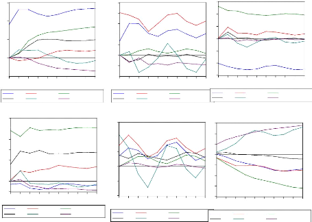
Response of LM2 to Cholesky

LPIBC LTCUSD

One S.D. Innovations

Response of LPIBC to Cholesky
One S.D. Innovations

LIPC LMARKUP LEXCESS_MONEY

LM2

Response of LTCUSD to Cholesky
One S.D. Innovations

1 2 3 4 5 6 7 8 9 10

1 2 3 4 5 6 7 8 9 10

1 2 3 4 5 6 7 8 9 10

.08

.06

.04

.02

.00

-.02

-.04

.06

.04

.02

.00

-.02

-.04

-.06

.10

.03

.02

.01

.00

-.01

LIPC LMARKUP LEXCESS_MONEY

LM2 LPIBC LTCUSD

LIPC LMARKUP LEXCESS_MONE

LM2 LPIBC LTCUSD

1 2 3 4 5 6 7 8 9 10

1 2 3 4 5 6 7 8 9 10

.06

.05

.04

.03

.02

.01

.00

-.01

.06

.04

.02

.00

-.02

-.04

-.01

-.02

-.03

-.04

.03

.02

.01

.00

1 2 3 4 5 6 7 8 9 10

LIPC LMARKUP LEXCESS_MONE

LM2 LPIBC LTCUSD

LIPC LMARKUP LEXCESS_MONEY

LM2 LPIBC LTCUSD

LIPC LMARKUP LEXCESS_MONEY

LM2 LPIBC LTCUSD

The shock is positive on LIPC generated by the negative effect of money supply, exchange rate, interest rate, and nominal GDP as seen above (seen figure 14) then the shock is negative to LIPC generated to positive effect of previews price level and mark up the whole fructuation on any variable have a significant impart on price level the figure above shows how change is made by mark up, excess money supply, money demand and GDP every period.

ition

The aim of decomposition of the variance of errors of prevision is to calculate for each innovation have as contribution on the errors variance expressed in percentage, when the innovation explain the big part in variance of error we conclude that the considered economy is sensible on shock which affect the series seen the appendix 5. The decomposition of the variance show that the variance of error prevision of the LIPC is due to 80% on its own innovation, 1% of the mark up innovation,10% of excess money supply innovation, 7% of M2 innovation ,1% of GDP innovation and 2% of exchange rate innovation.

The variance of error of the others variable is represented on the appendix 5 all of them show the accuracy.

.3.3.2.2 Forecast results

The forecast was produced using the data available through the first quarter of 1995. Table 16 provides the numeric forecasts both quarter-by-quarter and on an annual basis. The annual values for the levels of real GDP, nominal M2, and the two interest rate series are four-quarter averages. The annual values for the inflation rates and growth rates are measured on a fourth-quarter to fourth-quarter basis. Real growth for the third quarter of 2009 is forecast to be very slow, indeed to decline from the rate of 2010.1. In retrospect we know that this was a really large forecast error, since the third quarter of 2009 came in exceptionally strong. The forecast is for continued slow real growth (< 1 percent per quarter) though the end of 2010. This certainly will be an underestimate of real growth for 2009, and appears at this time (January, 2010) to be an underestimate of real growth for 2010.

In addition, the forecast did not catch the large increase in long rates and the accompanying increase in the slope of the yield curve that began in the last part of the 2010:1 and continued through third quarterly. In comparison, the money supply (M2) is projected to remain essentially constant through 2009 (around 6.10 percent), not far from the actual experience. Thus the long-term rate forecast errors in 2010 are attributable to errors in the implicit short-run term structure relationship. Taken literally, the model is forecasting a reduction in the exchange rate target to around

10. Finally, the model projects no change in the

o inflation rates (at roughly 2.5 percent per annum in terms of the CPI inflation rate) through the end of 2010. Hence the model is not predicting any increase in the long-run rate of inflation over this period.

Table 15: Prevision results

period	ipc	Lmarkup	Lexcess money	Lm2	lpibc	ltcusd
2009 q3	0.648560	0.184016	0.200919	6.078984	29.08976	6.370031
2009q4	0.538254	0.016532	0.262129	6.431286	29.28959	6.331708
2010q1	0.564918	0.297554	0.464941	6.664537	28.93297	6.303760
2010q2	0.621301	0.263436	0.607381	6.931436	29.97537	6.221759
2010q3	0.886635	0.114588	0.73921	6.506427	29.03635	6.295411
2010q4	0.701047	0.234921	0.499361	6.863611	29.95079	6.204930

The table15 above show the prevision of future variables and demonstrate how change will have the price level due to change of other variables here the variable are in percentage change. For example to comparing two period in 2^nd quarterly of 2009 inflation was 185.30 expressed as CPI and 3^rd quarterly the price level is 185.75 mean the evolution of 0.65% per/quarterly, the price level in 4^th quarterly will be 186.04 mean evolution of 0.54%, the price level of 1^st quarterly 2010 will be 186.38 mean evolution of 0.62% per quarterly, in the 2^nd quarterly of 2010 the price level will be 186.86 mean evolution of 0.89% per period and the 3^rd quarterly price level will be 187.23 mean the evolution of 0.7% per period. These fluctuations are results of demand shocks on one hand and the supply shocks on other.

model for forecasting because there are weighted sums (linear combinations) that are mean reverting (driven only by transitory shocks), as cointegrated variables and each variables is individually driven by permanent shocks, are cointegrated if and only if there exists a Vector Error Correction representation of the data series Nelson and Plosser (1982). The VECM has predicted inflation reasonably well over history and still appears to be a good forecasting model, especially in light of modifications like using adjusted, identifying policy shocks, and deriving probabilities for inflation outcomes.

The Rwanda inflation is driven in great part by the increase in money supply as it have been seen above but the excess money supply doesn't have the direct impact on price level its act through the exchange rate, and interest rate channel. These results provide useful insights into the behavior of inflation in Rwanda and the role of the National Bank of Rwanda in its determination. Inflation appears to be driven by both foreign and domestic factors in a manner consistent with conventional theoretical models and our understanding of the institutional structure of Rwanda economy. The results suggest that maintaining low inflation in coming years will depend largely on low level of interest rate, import, oil products in partner's countries and moderate growth of money supply and domestic unit labour costs. We have analyzed the inflation in two ways; first by the demand side as demand push inflation and on other hands by the supply side as cost push inflation.

1. On demand side for its part, the Rwanda national bank will need to maintain monetary conditions consistent with low inflation and low inflation expectations. In part, this is done through the pegged exchange rate, which acts as a nominal anchor for the economy. In this paper we wanted to analyze the driving forces of inflation process in Rwanda as a transition economy. First we derived, according to the theory, long-run sectoral relationship affecting inflation (markup, excess money, nominal exchange rate and GDP). Then we estimated short-run structural inflation function by imposing above mentioned long-run relationships together with various short-run variables which might contribute to explaining the inflation process in Rwanda, we conclude that inflation in Rwanda rise when money supply increase this by the increase in aggregate demande due also by the increased private and government spending.

2. On the supply side the mark up is seen to be significant because the increase of oil price, and import price increase at the sime time and immediately the price of domestic goods. As economic policy which is liberalized the producers to whom the oil is part of their cost could then pass (this change in price level) on to consumers in the form of increased price. In the derive quarterly ahead model of inflation, we found that all long run relationships except GDP significantly influence quarter-on-quarter

monetary variables are found to be important in

ar as narrow monetary aggregate is concerned, one can notice that the magnitude of its influence on consumer price inflation is quite marginal.

For forecast purpose we designed ECM model first by Hendry equations is not a perfect one, secondly by Engle Granger which proven instable by forecast criteria this is because of a high number of parameters estimated, while the definability of some equations is relatively high (a low relative coefficient of determination). However, they may be applied to the forecasting of inflation because the mean square errors of the forecast conform to the selected minimum criteria (1 or 5% should be mentioned). One of the main drawbacks of the VECM model, where the VAR methodology is used, is the fact that each time additional observations appear and the model is estimated as new equation of each group may be complemented (or reduced) by different variables. However, given stable parameters, the accuracy of results is not damaged. Nevertheless, the designing of a structural VAR or multi-equation econometric model for the forecasting of the CPI should probably be considered in future.

The VECM has predicted inflation reasonably well over history and still appears to be a good forecasting model, especially in light of modifications like using adjusted, identifying policy shocks, and deriving probabilities for inflation outcomes. Forecasts from the VECM can augment the information coming from other models used at the Bank. They can provide alternative views of what could happen in the economy and give some information about the «balance of risks.» Multiple models could be especially helpful to policy-makers during times of extreme uncertainty and/or structural shifts, but even in relatively stable times, advice from different models helps to balance risks about the outlook for the future.

According to the accuracy of the forecast calculated by the VECM model, this model could be suggested as a tool applied by the economists-analysts in the decision making procedure.

Some caveats are in order. First, the approach in this paper has been to evaluate forecasting performance using a simulated out of sample methodology. This methodology provides a degree of protection against overfitting and detects model instability. However, because a large number of forecasts were used, some over fitting bias nonetheless remains. This suggests that some of the best-performing forecasts produced using individual economic indicators might deteriorate as one move beyond the end of our sample. That is why the model used here could be improved in the future because;

- Coefficients of predictors can change over time

- The number of predictors can be large

- The relevant model for forecasting can potentially change over time

- The variables can also change over time

Second, we have considered only linear models. To the extent that the relation between inflation and some of the candidate variables is nonlinear, these results understate the forecasting improvements that might be obtained. Moreover, with few exceptions, incorporating other variables could be necessary to improve upon the short run forecasts and must be considered by National Bank agent in their future research.

1. Adam Smith. (1776), «Wealth of nations»

2. Ando, A. and F. Modigliani (1963), «The `Life-Cycle' Hypothesis of Saving: aggregate Implications and Tests», American Economic Review.

3. Banerjee, A., J. Dolado, J.W. Galbraith and D.H. Hendry (1993). Co-integration, Error-Correction, and the Econometric Analysis of Non-Stationary Data, Oxford University Press, Oxford.

4. Bewley, R.A. (1979). The Direct Estimation of the Equilibrium Response in a Linear Dynamic Model, Economic Letters.

5. Bomhoff, E.J. (1991). Inflation in Western Europe, paper prepared for the Fifth International Conference sponsored by the Institute for Monetary and Economic Studies, Bank of Japan, October.

6. Campbell, J.Y. and R.J. Shiller (1987),»Cointegration and tests of Present value Models» Journal of political Economy, 95

7. Duesenberry, J. (1950). The Mechanics of Inflation, Review of Economics and Statistics, 32 (2).

8. Edwards, Sebastian. (2002), «The great exchange rate debate after Argentina», The North American Journal of Economics and finance, Volume 13, Issue 3

9. Engle, R.F. and C.W.J. Granger (1987), «Cointegration and Error Correction: Representation, Estimation, and Testing» Econometrica, 55

10. Gary K. and Dimitris K, (2009), Forecasting Inflation Using Dynamic Model Averaging University of Strathclyde, June 2009

Principle of forecasting; A handbook for

A

12. Kiley, Michel J. (2008). «Estimating the common trend rate of inflation for consumer prices and consumer prices excluding food and energy prices». Federal reserve Board.

13. Klein, L.R. and R. F. Kosobud (1961), «Some Econometrics of Growth: Great Ratios of Economics», Quarterly Journal of Economics, 75

14. Kremers, J.J.M., N.R. Ericsson and J.J. Dolado (1992). The Power of Cointegration Tests, Oxford Bulletin of Economics and Statistics, 54 (3)

15. Mankiw, N.G.(1998) «Economic principles». New York: university Publishers,de Croisillon de Harcourt.

16. Mishkin, F. S. (1992), Is the Fisher effect for real: A reexamination of the relationship between Inflation and Interest rates, Journal of Monetary Economics 30

17. Murray, M. P(1994), «A drunk and her dog: An illustration of cointegration and error correction,» American Statistician, 48

18. Paul H. Walgenbach, Norman E. Dittrich and Ernest I. Hanson,(1973).»The Measuring Unit principle»

19. Payne, James E., (2002), «Inflationary Dynamics of a Transition Economy: the Croatian Experience», Journal of Policy Modeling, 24(3),

20. Sargent, Thomas J. (1986), «Rational Expectations and Inflation», New York; Harper and Row.

21. Selgin, G.A,(1989) «The analytical Framework of real bill Doctrine» Journal of institutional and theoretical economics, Volume 145,

22. Stock J. and Watson M. (1999), Forecasting inflation. Journal of Monetary Economics 44,

2001) : Research methodology course for the es , 2^nd edition , Paris, Durod

Working Papers

1. Bandawe, H.P. (1997). Causes of Inflation in Fiji: Experience during 1979-1994, working Paper, Reserve Bank of Fiji.

2. Brower, G. and N.R. Ericsson (1995). Modeling Inflation in Australia, Reserve Bank of Australia, Research discussion Paper No. 9510

3. Debelle, G. and G. Stevens (1995). Monetary Policy Goals for Inflation in Australia, Reserve Bank of Australia, Research Discussion Paper No. 9530.

4. Jean Claude Trichet, (2004), Federal reserve board's semiannual Monetary Policy Report to the congress round table, July 1, 2004

5. Morling, S. (1997). Modeling Inflation in Fiji, Working Paper, Reserve Bank of Fiji.

APPENDIX 1: DATA DEFINITIONS

This appendix describes the data. The list the definitions of the data and give their sources. All data are quarterly, and the sample period is 1995(1)-2009(2).

2. Consumer Price Index (IPC)

Definition: The Consumer Price Index is a Laspeyres index that covers household consumption as it is used by national accounts. The reference population for the CPI consists of all households living in urban areas in Rwanda. The household basket includes 438 products observed in many places spread all over the administrative centers of all provinces in Rwanda. All kinds of places of observation are selected: shops, markets, services, etc. More than 25,000 prices are collected every month by enumerators of the National Institute of Statistics of Rwanda and of the National Bank of Rwanda. The base year for the CPI is the year 2003. The weights used for this new index are the result of the Household Living Conditions Survey (EICV) conducted in 2000-2001 with a sample of 6,450 households. The splicing with the old index is feasible using the splicing coefficient of 3.889. If you divide the old index by this coefficient, you will be able to make comparisons with the new index based in 2003.

The consumer price index is calculated by the RNIS and published every quarterly the base is 2003=100 (NISR) is adjusted.

Source: National Institute of Statistics of Rwanda (NISR), P.O. BOX 6139 Kigali,

Tel.: [phone] Fax: [phone], Web site: www.statistics.gov.rw /CPI Indexes

3. Unit Labour Costs (ULC)

Definition: Nominal cost of all labour per unit of output.

Nominal unit labour costs are defined as:

salaries + payroll taxes - employment subsidies divided by gross domestic product Where salaries refers to the wages, salaries and supplements of all employee in public and private sector including volontaries wage and salary earners. The class «wage and salary earners» is only a subset of all employed people in the economy,

f-employed, employers. Unit labour costs of wage

scaled up to that by adding the 5% as legal percentage of ratio payed in national social security fund( NSSF).

Source: Author calculation using then NSSF data.

4. Import Prices (IP)

Definition: The NBR publish every month the quantity of goods imported and they values, using these data we calculate the import price index of merchandise imports, excluding without the oil import items. Import prices are measured as the implicit price on seasonally adjusted merchandise imports, excluding exogenous imports. Exogenous imports are goods which are lumpy in nature, subject to government arrangements or significantly affected by factors other than the general level of economic activity in Rwanda. Specifically, this covers fuel, defense equipment, and ships, aircraft and other large items of equipment acquired by selected public and private enterprises.

The monthly data are adjusted on quarterly basis using the moving average, Author calculation

Source: NBR, Foreign Exchange Inspection and Balance of Payments Department

5. Petrol Prices (PP)

Definition: Automotive fuel price index or oil price index.

On the monthly basis the NBR publish the quantity and the values of energy and lubricant which include piles and electrics accumulators, fuels, gaz oils, lubricating oils and others fuels products using these available data we calculate the oil price index on Layperes basis and finally adjusted on quarterly.

Source: NBR, Foreign Exchange Inspection and Balance of Payments Department 5. M2

Definition: M2 is the monetary base which include the currency in circulation plus
commercial bank reserves at the central bank this mean M1( currency in circulation

nd saving deposit which is published by the national s deflated using the current CPI.

Source: NBR, Research department.

6. The exchange rate (TCUSD)

Definition: The nominal exchange rate used in the study is defined as unit of Rwanda franc per United States dollar. The basic calculation is made by dairly basis and later adjusted on the quarterly base.

Source: NBR, Foreign Exchange Inspection and Balance of Payments Department

7. Interest rate (TDC)

Definition: The interest rate represents the spread between the 91-day treasury bills and the average annual interest offered on time and saving deposit and this spread represent the return on domestic financial assets. The interest rate of central has been used as the measure of the spread.

Source: NBR, Foreign Exchange Inspection and Balance of Payments Department

8. The nominal GDP

The GDP represent the national output is published on the year basis we estimated it using the eviews to get the quarterly data. This involves adjusting a linear interpolation of annual GDP series with weigthed percentage errors between actual quarterly data. Then the resulting was seasonally adjusted to minimize the impact of the cyclical components.

PIB	ULC	IP	TCUSD	OIL PRICE INDEX
72.90	0.0064	1082168	172.99	341.84
81.60	0.0063	810447	273.42	347.02
89.00	0.0062	1265720	312.94	339.49
95.50	0.0069	1092288	304.43	439.08
96.10	0.0072	986104	305.16	315.97
102.20	0.0075	3478570	307.14	339.08
109.00	0.0072	663810	306.94	315.97
116.70	0.0072	606585	307.42	315.89
129.70	0.0065	282688	305.35	318.2
137.00	0.0062	329202	301.67	310.61
143.20	0.0063	265033	299.65	319.95
148.30	0.0064	309131	304.13	319.95
150.90	0.0063	317448	307.25	326.39
154.30	0.0063	292589	309.30	328.44
156.90	0.0062	361544	315.44	350.65
159.10	0.0067	359701	325.17	373.87
157.50	0.0069	330049	332.73	403.09
162.20	0.0071	338890	335.24	410.89
165.50	0.0070	319282	334.18	437.56
171.10	0.0076	368840	342.67	458.61
174.80	0.0075	434809	362.87	454.38
178.20	0.0076	377019	379.39	457.77
181.50	0.0076	356082	405.45	459.32
183.10	0.0081	335797	425.22	461.17
186.50	0.0076	394560	433.65	466.04
190.20	0.0076	361482	439.91	466.43
194.30	0.0076	304842	444.86	495.12
199.20	0.0079	329135	456.52	496.18
203.80	0.0081	310087	460.78	517.58
208.40	0.0082	372846	466.90	532.32
213.40	0.0083	395299	482.01	533.5
216.00	0.0087	395426	502.01	563.25
222.20	0.0090	454943	513.80	517.2
229.30	0.0091	430441	531.69	493.6
237.60	0.0090	495160	550.98	500.8
249.70	0.0094	485623	570.24	497.0
259.10	0.0100	455757	582.43	459.5
268.10	0.0099	462887	579.73	388.3
277.20	0.0098	466906	576.23	386.9
285.40	0.0100	593191	568.84	361.7
294.60	0.0098	507757	562.92	420.4

TDC

IPC

PERIOD M2

39.80	10.04	-
49.74	12.06	61.87
59.27	12.04	70.80
62.64	12.12	71.73
62.13	9.00	70.90
64.58	9.36	71.10
66.60	9.43	74.40
68.87	11.26	76.33
74.14	8.39	77.63
84.29	9.07	78.40
81.11	8.52	81.43
88.60	8.24	88.10
85.45	9.94	88.77
82.66	9.21	89.27
84.18	9.16	86.20
91.99	7.76	84.47
102.79	7.91	84.90
103.04	9.19	83.93
107.38	8.53	85.00
102.51	8.75	86.00
103.80	9.20	86.23
109.72	9.44	86.93
107.36	9.41	88.57
119.39	10.11	91.47
122.17	9.69	92.03
127.75	10.16	91.13
125.32	9.91	90.90
130.69	10.18	91.07
129.70	10.15	91.20
135.60	10.00	91.80
135.30	9.34	93.53
144.31	9.10	95.80
143.25	8.94	96.87
145.89	9.11	98.87
158.31	9.27	100.83
167.53	9.33	103.43
162.41	8.91	107.24
161.28	9.26	109.82
167.25	9.33	113.56
187.23	9.43	117.18
190.84	13.50	120.06

1995-1

1996-1

1997-1

1998-1

1999-1

2000-1

2001-1

2002-1

2003-1

2004-1

2005-1

				122.70
				123.39
				122.49
220.07		8.08		128.01
237.64		8.18		132.81
254.15		8.32		134.84
285.98		8.24		136.24
273.63		7.90		143.08
301.76		7.69		144.33
326.77		7.57		145.81
375.27		7.32		146.91
422.16		7.56		152.70
445.39		8.21		163.03
465.03		10.10		174.40
468.16		9.23		179.40
468.16		7.90		181.90
468.00		8.10		185.30
303.70	0.0099		549816		556.99		320.1
313.20	0.0095		511935		554.44		230.2
322.20	0.0099		519140		553.73		371.5
332.10	0.0108		486034		553.86		506.3
342.10	0.0109		541193		552.04		364.5
352.80	0.0118		439671		551.29		345.5
358.60	0.0125		452765		550.01		328.4
354.20	0.0135		411030		547.87		399.4
371.85	0.0136		439717		546.37		357.8
387.76	0.0133		556641		547.89		444.5
403.46	0.0137		504527		545.12		605.5
419.54	0.0138		594475		543.89		574.8
517.68	0.0118		755817		543.35		645.4
500.73	0.0126		771322		547.13		574.8
451.19	0.0150		778,849		553.01		621.7
369.12	0.0177		773299		566.00		605.5
515.22	0.0132		721312		572.30		532.0

2006-1

2007-1

2008-1

2009-1

2009-2

APPENDIX 3: RESIDUALS PROPERTIES

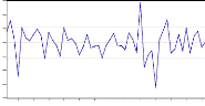
1996 1998 2000 2002 2004 2006 2008

.06

.04

.02

.00

-.02

-.04

-.06

.3

.2

.1

.0

-.1

-.2

-.3

-.4

.10
.05
.00

-.05
-.10
-.15

.2

.1

.0

-.1

-.2

DLPIBC Residuals

DLIPC Residuals

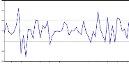
1996 1998 2000 2002 2004 2006 2008

DLTDC Residuals

DLM2 Residuals

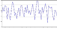
1996 1998 2000 2002 2004 2006 2008

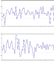
1996 1998 2000 2002 2004 2006 2008

DLTCUSD Residuals

DLULC Residuals

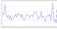
1996 1998 2000 2002 2004 2006 2008

1996 1998 2000 2002 2004 2006 2008

.20
.15
.10

.05
.00

-.05
-.10
-.15

.03

.02

.01

.00

-.01

-.02

-.03

Page 71

Vector Autoregression Estimates

Date: 11/22/09 Time: 11:49

Sample (adjusted): 1995Q4 2009Q2

Included observations: 55 after adjustments Standard errors in ( ) & t-statistics in [ ]

LIPC

LIPC(-1) 1.101540

(0.26175)

[ 4.20837]

LIPC(-2) -0.422070

(0.27787)

[-1.51896]

LMARKUP(-1) -0.056816

(0.03854)

[-1.47435]

LMARKUP(-2) 0.013979

(0.03739)

[ 0.37387]

LEXCESS_MONEY(

-1) -0.083627
(0.13791) [-0.60639]

LEXCESS_MONEY(

-2) -0.027293
(0.14280) [-0.19113]

LM2(-1) 0.111751

(0.14672)

[ 0.76165]

LM2(-2) 0.031747

(0.16028)

[ 0.19807]

LPIBC(-1) 0.089677

(0.06716)

[ 1.33521]

LEXCESS_

LMARKUP MONEY			LM2	LPIBC	LTCUSD
2.141111	-2.130141		-1.578700	-1.192560	-0.352104
(1.26259)	(0.84661)		(0.65981)	(0.84264)	(0.17829)
[ 1.69581]	[-2.51609]		[-2.39264]	[-1.41526]	[-1.97489]
-3.151490	1.704996		1.269049	-0.239753	0.231334
(1.34034)	(0.89874)		(0.70045)	(0.89453)	(0.18927)
[-2.35127]	[ 1.89709]		[ 1.81177]	[-0.26802]	[ 1.22224]
0.450103	0.170646		0.012606	0.227207	-0.033242
(0.18589)	(0.12464)		(0.09714)	(0.12406)	(0.02625)
[ 2.42140]	[ 1.36908]		[ 0.12977]	[ 1.83144]	[-1.26640]
0.231217	-0.193665		-0.092581	0.010903	-0.035885
(0.18035)	(0.12093)		(0.09425)	(0.12037)	(0.02547)
[ 1.28204]	[-1.60144]		[-0.98230]	[ 0.09058]	[-1.40905]
0.564419 (0.66523) [ 0.84845]	0.032940 (0.44606) [ 0.07385]	-0.761326 (0.34764) [-2.18996]		-0.568270 (0.44397) [-1.27997]	-0.026493 (0.09394) [-0.28202]
-1.341830	0.298516	0.279204		-0.394038	0.055375
(0.68882)	(0.46187)	(0.35997)		(0.45971)	(0.09727)
[-1.94802]	[ 0.64631]	[ 0.77563]		[-0.85714]	[ 0.56931]
-0.810507	0.660783	1.492038		0.765855	-0.076622
(0.70774)	(0.47456)	(0.36986)		(0.47234)	(0.09994)
[-1.14521]	[ 1.39241]	[ 4.03410]		[ 1.62141]	[-0.76668]
1.375501	-0.332027	-0.249299		0.523881	0.027241
(0.77313)	(0.51841)	(0.40403)		(0.51598)	(0.10917)
[ 1.77914]	[-0.64047]	[-0.61704]		[ 1.01531]	[ 0.24952]
-0.013350	0.295970	0.442492		0.448134	0.010639
(0.32397)	(0.21723)	(0.16930)		(0.21622)	(0.04575)
[-0.04121]	[ 1.36245]	[ 2.61359]		[ 2.07261]	[ 0.23257]

LTCUSD(-1) -0.281546

(0.14066)

[-2.00166]

LTCUSD(-2) 0.222899

(0.13707)

[ 1.62619]

C -1.676818

(1.69667)

[-0.98830]

R-squared 0.996371

Adj. R-squared 0.995334

Sum sq. resids 0.013769

S.E. equation 0.018106

F-statistic 960.8409

Log likelihood 150.0073

Akaike AIC -4.982082

Schwarz SC -4.507621

Mean dependent 0.043181

S.D. dependent 0.265052

-0.016498	-0.358248	-0.444169	-0.358673	0.176711
(0.43672)	(0.29283)	(0.22822)	(0.29146)	(0.06167)
[-0.03778]	[-1.22338]	[-1.94619]	[-1.23059]	[ 2.86547]
-0.974949	0.733304	0.431368	0.233600	1.218535
(0.67847)	(0.45494)	(0.35456)	(0.45281)	(0.09581)
[-1.43697]	[ 1.61187]	[ 1.21662]	[ 0.51589]	[ 12.7186]
0.800388	-0.862067	-0.552112	-0.127980	-0.311163
(0.66117)	(0.44334)	(0.34552)	(0.44126)	(0.09336)
[ 1.21056]	[-1.94450]	[-1.59792]	[-0.29003]	[-3.33279]
-0.864729	0.918994	-0.389253	18.86430	-4.492430
(8.18413)	(5.48774)	(4.27694)	(5.46204)	(1.15568)
[-0.10566]	[ 0.16746]	[-0.09101]	[ 3.45371]	[-3.88725]
0.737300	0.627502	0.995287	0.986779	0.998160
0.662242	0.521074	0.993941	0.983002	0.997634
0.320365	0.144041	0.087492	0.142695	0.006388
0.087337	0.058562	0.045641	0.058288	0.012333
9.823162	5.896025	739.2045	261.2321	1898.408
63.46310	85.44554	99.15586	85.70373	171.1258
-1.835022	-2.634383	-3.132941	-2.643772	-5.750031
-1.360561	-2.159923	-2.658480	-2.169312	-5.275570
0.014606	-0.001208	5.025937	28.44066	6.090165
0.150278	0.084622	0.586355	0.447072	0.253544

[-0.47015]

Determinant resid covariance
(dof adj.)	4.13E-19
Determinant resid covariance	8.19E-20
Log likelihood	740.3481
Akaike information criterion	-24.08538
Schwarz criterion	-21.23862

Appendix 5: Variance decomposition of VECM

Variance Decomposition of LIPC: Perio d S.E. LIPC LMARKUP				LEXCESS _ MONEY	LM2	LPIBC	LTCUSD
1	0.018297	100.0000	0.000000	0.000000	0.000000	0.000000	0.000000
2	0.032540	96.90690	0.261702	0.595329	0.499544	1.721004	0.015519
3	0.043520	90.62316	0.191614	4.832142	2.512064	1.817140	0.023875
4	0.052351	83.63004	0.136518	8.777639	5.243455	1.894989	0.317361
5	0.059778	78.48380	0.195292	12.07487	6.924228	1.525553	0.796257
6	0.066923	75.02531	0.419849	14.20681	7.772816	1.218449	1.356770
7	0.074009	72.88328	0.648207	15.70749	7.907380	1.077777	1.775871
8	0.081031	71.31248	0.750457	16.86669	7.916372	1.034312	2.119692
9	0.087759	70.04459	0.799915	17.85948	7.905447	0.980837	2.409730

74863 18.69154 7.959918 0.875919 2.673639

RKUP:

LEXCESS

MONEY LM2 LPIBC LTCUSD

Perio

d S.E. LIPC LMARKUP

_

1	0.085733	10.12798	89.87202	0.000000	0.000000	0.000000	0.000000
2	0.131525	25.71178	72.02151	0.006302	0.899849	0.264277	1.096287
3	0.163858	29.98207	63.86561	0.275853	0.849396	4.217105	0.809964
4	0.177746	30.92442	60.75896	0.698480	0.730917	5.229595	1.657623
5	0.192141	29.93022	62.02403	0.724407	0.649359	4.550724	2.121260
6	0.214214	28.82513	62.77342	0.613363	0.525383	4.773778	2.488929
7	0.234401	28.50856	63.99687	0.619720	0.452586	3.987878	2.434389
8	0.248487	27.96734	63.66144	0.782854	0.407589	4.605363	2.575415
9	0.259852	27.17995	63.00427	0.842011	0.383605	5.795693	2.794468
10	0.271840	27.12109	63.31215	0.786374	0.399906	5.369609	3.010871

Variance Decomposition of LEXCESS_MONEY:

Perio d		S.E.	LIPC		LMARKUP	LEXCESS _ MONEY	LM2	LPIBC	LTCUSD
1		0.066526	37.38368		0.041603	62.57472	0.000000	0.000000	0.000000
2		0.095655	40.93250		3.918057	53.35775	1.232881	0.537617	0.021192
3		0.117338	44.87656		3.191635	50.20760	0.825644	0.747469	0.151092
4		0.135264	47.85993		2.807033	46.95173	0.631856	1.615467	0.133980
5		0.149603	50.12986		2.460321	45.22608	0.531474	1.481649	0.170621
6		0.161253	50.98821		2.647058	44.45449	0.484415	1.275346	0.150483
7		0.171989	51.31621		2.706138	44.27728	0.428598	1.134399	0.137376
8		0.183281	51.89167		2.584419	43.92870	0.377480	1.096480	0.121256
9		0.194634	52.81078		2.376649	43.25861	0.336331	1.102984	0.114654
10		0.204847	53.63574		2.288540	42.62055	0.306779	1.039664	0.108725
Variance Decomposition of LM2: Perio d S.E. LIPC LMARKUP						LEXCESS _ MONEY	LM2	LPIBC	LTCUSD
1	0.051043			0.350690	0.055566	89.42647	10.16727	0.000000	0.000000
2	0.073794			0.264612	1.755991	76.19698	19.86784	1.871757	0.042818
3	0.094336			0.678710	1.849955	75.90141	20.13481	1.184020	0.251098
4	0.111029			0.990596	2.250991	73.81612	21.58103	0.911013	0.450254
5	0.125225			1.091928	2.660878	73.37158	21.37689	0.776895	0.721820
6	0.137984			0.961006	3.373420	72.87852	21.27225	0.652282	0.862522
7	0.150007			0.835199	3.709558	72.80418	21.07802	0.593375	0.979670
8	0.161627			0.761029	3.813367	72.71875	21.01232	0.633132	1.061403
9	0.172552			0.731259	3.834466	72.64545	20.98426	0.636342	1.168230
10	0.182762			0.693408	3.985485	72.54635	20.92388	0.593409	1.257465

Variance Decomposition of LPIBC:

Perio

d S.E. LIPC LMARKUP

LEXCESS

MONEY LM2 LPIBC LTCUSD

_

22762
29179
04580

4 0.098952 14.50754 37.38808

5 0.102642 15.49777 38.18783

6 0.116172 18.32080 38.82996

7 0.130118 20.95032 39.69009

8 0.136354 21.16591 39.71859

9 0.140460 20.28022 39.00492

10 0.143889 20.17289 40.02714

0.000290	7.565386	59.66085	0.000000
0.689948	5.504930	39.01509	0.361021
2.706326	7.924112	31.11456	0.446975
4.071785	8.757723	34.88760	0.387276
4.196817	9.282737	32.44972	0.385130
3.372594	7.782297	31.39360	0.300751
3.178140	7.329111	28.57389	0.278452
4.142156	8.617926	26.08331	0.272105
4.870003	9.756058	25.82769	0.261103
4.902321	10.00941	24.61460	0.273639

Variance Decomposition of

LTCUSD:

Period LEXCESS

S.E. LIPC LMARKUP MONEY LM2 LPIBC LTCUSD

_

1	0.011168	0.173076	7.267890	8.255018	1.279036	4.236467	78.78851
2	0.022223	1.053871	11.07978	18.00470	1.116873	7.527846	61.21693
3	0.035166	3.220732	13.36857	23.19984	0.463252	12.33115	47.41645
4	0.050203	4.226496	10.96903	26.08153	0.228007	20.42038	38.07456
5	0.065036	4.829875	9.019364	27.59094	0.143855	24.71258	33.70338
6	0.078331	5.752720	8.409146	29.00032	0.109422	24.39696	32.33143
7	0.090758	6.952437	8.811006	30.28924	0.113849	22.24306	31.59041
8	0.103117	7.713250	9.178553	31.46720	0.170577	20.71041	30.76000
9	0.115532	7.744092	9.075099	32.37502	0.258851	20.64557	29.90137
10	0.127537	7.499270	8.803140	32.89073	0.319129	21.15154	29.33619

Cholesky Ordering: LIPC LMARKUP LEXCESS_MONEY LM2
LPIBC LTCUSD

its test

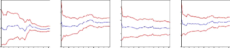
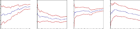
1.5 1.0 0.5 0.0 -0.5

-1.0

00 01 02 03 04 05 06 07 08

Recursive C(1) Estimates #177; 2 S.E.

.05 .00 -.05 -.10 -.15 -.20 -.25

-.30

00 01 02 03 04 05 06 07 08

.2 .0 -.2 -.4

-.6

00 01 02 03 04 05 06 07 08

Recursive C(2) Estimates #177; 2 S.E.

.6 .4 .2 .0

-.2

00 01 02 03 04 05 06 07 08

.25 .20 .15 .10 .05 .00 -.05

-.10

00 01 02 03 04 05 06 07 08

Recursive C(3) Estimates #177; 2 S.E.

.2
.1
.0

-.1

-.2

-.3

00 01 02 03 04 05 06 07 08

0.4 0.0 -0.4 -0.8

-1.2

00 01 02 03 04 05 06 07 08

Recursive C(4) Estimates #177; 2 S.E.

.6 .4 .2 .0 -.2

-.4

00 01 02 03 04 05 06 07 08

Recursive C(5) Estimates #177; 2 S.E.

Recursive C(6) Estimates #177; 2 S.E.

Recursive C(7) Estimates #177; 2 S.E.

Recursive C(8) Estimates #177; 2 S.E.

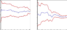
.8 .4 .0 -.4

-.8

Recursive C(9) Estimates #177; 2 S.E.

00 01 02 03 04 05 06 07 08

.3 .2 .1 .0

-.1

-.2

Recursive C(10) Estimates #177; 2 S.E.

00 01 02 03 04 05 06 07 08