Modeling and forecasting inflation in Rwanda (1995-2009)( Télécharger le fichier original )par Ferdinand GAKUBA Kigali Independent University - Degree in economics 2009 |

2.4 THE LONG RUN MODEL OF INFLATIONVarious economists have attempted to empirically analyze the
issues outlined in the
e found that monetary disequilibrium and exchange xplaining the behaviour of prices in the Jamaican economy46. The link between the money stock and inflation occurs via a monetary transmission process whereby the amount of money economic agents desire to hold is less than the available money stock. Assuming a stable demand for money, this serves to reduce the value of money (in terms of goods) thus increasing the price level. We estimated a model similar to the Harberger model using ordinary least squares. The results using quarterly are; DLIPC = 0.104*LEXCESS_MONEY(-1) + 0.062*LMARKUP + 0.099*DLM2 - 0.0327*DLOPC + 0.20*DLPIBC + 0.21*DLTCUSD(-1) - 0.0034*DLTDC(-1) + 0.184*DLULC - 0.0067*DLIP With R-squared= 0.42, Schwarz criterio=-4,38, F-statist= 1,23 ,DW= 1.25, Chow = 1.11, Normality test= 1,32 and ARCH= 0.38 sigma= 0.96 We estimated a general model in which we regressed Dlcpi (difference in logarithm of consumer price index) on the above mentioned long run (and structural) relationships markup,Lexcess_moneyt-1, and Dlpibc, and short run dynamics Dltcusd(-1), Dlulc, Dlip, DLm2 and DLtdc Our sample goes from 1995Q1 until 2009Q2 and for that sample period our unrestricted general model yields sigma = 0.96 percent for 9 regressors and 56 observations (Schwarz criterion = -4.38). Next step was eliminating insignificant terms from the model by allowing the log variables stationary The procedure followed is general to simple approach LIPC = 0.016*LIP(-1) + 0.81*LIPC(-1) + 0.121*LM2 - 0.047*LOPC - 0.025*LPIBC(- 1) + 0.020*DLTDC(-1) _ 0.077*DLULC(-1) + 0.406*DLTCUSD 46 Wayne Robinson (1998) : Forecasting inflation using VAR analysis, Bank of Jamaica
26 F-statistic= 1060,04 , Jarque- bera= 9.14,ARCH est with also high probability over 5%. The model proved its adequacy in terms of various diagnostic tests and also it encompasses the unrestricted general model. For more information see appendix 6 The contemporaneous money stock, import price, oil price, and exchange rate had expected signs and were very significant. The results suggest that the money supply, import prices, mainly the oil prices fluctuations and exchange rate changes had the largest impact on price changes. Using the quarterly data the model derived is; LIPC = 0.029 + 0.016* LIP t-1 + 0.81*LIPC t-1 + 0.121*LM2 -0.047* LOPC- 0.026* LPIBC t-1 +0.020* DLTDC t-1 - 0.077*DLULC t-1 +0.40*DLTCUSD Table 7: Results for long run inflation model Dependent Variable: LIPC Method: Least Squares Date: 11/06/09 Time: 09:41 Sample (adjusted): 1995Q3 2009Q2 Included observations: 56 after adjustments
ighly influenced by lagged inflation, money supply ese results also highlight the significant role of oil prices and import prices, starting from the hypothesis of the Quantity Theory, estimated the relationship between money supply and prices in Rwanda between 1995 and 2009. The changes in prices were examined as a function of changes in the money supply (M2), previous price changes and changes in the exchange rate. Using quarterly data, the estimated model most preferred was; LIPC = 0.029 + 0.016* LIP t-1 + 0.81*LIPC t-1 + 0.121*LM2 -0.047* LOPC- 0.026* LPIBC t-1 +0.020* DLTDC t-1 - 0.077*DLULC t-1 +0.40*DLTCUSD 2.4.1 Interpretation of coefficients R- squared= 99.44% this mean that the 99.44 % fluctuations of prices are explained by last inflation, money supply, exchange rate, import price and oil shocks. Most coefficients are statistically significant only the coefficients of LPIBC, DLTDC, and DLULC have a high probabilities the reason for that is because the PIBC was estimated for quarterly the ULC was calculated using NSSF data. This could lead to estimators bias. 2.4.2 Classical Tests -The T- Student of LIP t-1, LIPC t-1, LM2, LOPC and DLTCUSD have the significant influence on inflation. -Homocedasticity test of correlation of errors Ho= the model is homocedastic H1= the model is heteroscedastic Table 8: Heteroskedasticity test White heteroskedasticity test: No cross terms
With the two option test above we accept the first assumption that there is homoskedasticity because the probabilities are high than 5%
H1= errors correlated We dispose here the sample n= 56 observations. The number of real explanatory variables is K=8 on Durbin Watson table at 5% level of freedom; Dinf=1,39 and Dsup= 1,51 and our DW calculated is =1, 26 this mean that there is presumably a positive autocorrelation of errors. We correct the autocorrelation with the Cochrane Orcutt method by adding the inverted AR root The DW find after new estimation is= 1.68 and K have been 9 so Dinf =1,32 and Dsup= 1.58 mean that we presumably resolve the autocorrelation problems by Cochrone Orcutt method Ho is accepted no correlation among errors. Test of Ramsey RESET The assumptions for this test are as follows; Ho= the specification of model is good H1= the model is badly specified Table 9: Ramsey RESET test Ramsey RESET TEST
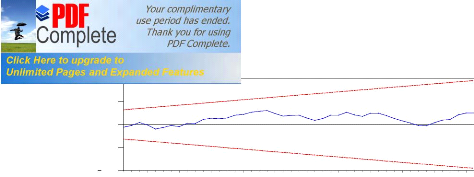
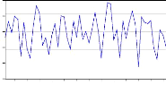
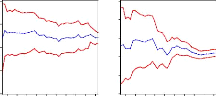
These two probability show that the model specification is good because the probalitity are higher than 5% mean that we accept Ho. Figure 5: CUSUM Test If the cusum curve is out of corridor means that the coefficients of the models are unstable and curve does not leave the corridor mean that the coefficients are stable.
0
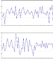
98 99 00 01 02 03 04 05 06 07 08 Figure 6: CUSUM squared test This test allow to detect the punctual instability
e ECM is instable the 2005-2006 is instable period. e unadequancy and is instable at certain period so due to lack of certain dummies variables which could be included to correct it, so we didn,t have during this estimation so we propose another ECM recommended by Engle- Granger with two-step. 3.2.2 The ECM with Engle - Granger The model of Granger enables the long-run equilibrium relationship and short-run dynamics to be estimated simultaneously particularly for finites samples, where ignoring dynamics when estimating the long run parameters can lead to substantial bias48. One of the advantages of this specification is that it isolates the speed of adjustment parameter C(9), which indicates how quickly the system returns to equilibrium after a random shock. The significance of the error correction coefficient is also a test for cointegration. Kremers, Ericsson and Dolado (1992) have shown this test to be more powerful than the Dickey-Fuller test applied to the residuals of a static long-run relationship. Another reparameterisation, the Bewley (1979) transformation, isolates the long-run or equilibrium parameters and provides t-statistics on those parameters. Inder (1991) shows these approximately normally distributed t-statistics are less biased than the Phillips-Hansen adjusted t-statistics The model is expressed as follow; DLIPC = C(1) + C(2)*LEXCESS_MONEY + C(3)*DLMARKUP + C(4)*RESID01(-1) + C(5)*LTDC(-1) + C(6)*DLM2(-2) + C(7)*LOPC(-1) + C(8)*DLTCUSD(-1) + C(9)*DLPIBC(-1) + C(10)*LULC(-1) The results for estimated model are as follow; DLIPC = -0.0199- 0.173*LEXCESS_MONEY + 0.038*DLMARKUP - 0.319*RESID01 (-1) - 0.030*LTDC (-1) + 0.067*DLM2 (-2) + 0.033*LOPC (-1) + 0.062*DLTCUSD (-1) + 0.165*DLPIBC (-1) + 0.019*LULC (-1) 48 Banerjee et al. (1993) and Inder (1994) show that substantial biases in static OLS estimates of the cointegration parameters can exist, particularly in finite samples, and the unrestricted error correction models can produce superior estimates of the cointegrating vector. e level of priced in Rwanda is negatively related to
between variables 3.2.2.1 Long-run elasticity and short run elasticity The short run elasticity is represented by 134 139 coefficients; if the level of money supply grow by 10% then the inflation rise by 0.067%, if the exchange rate fluctuate by 10% the inflation rise by 0.030%, If the oil price increase by 10% the inflation rise by 0.033%, if the salaries rise by 10% the inflation rise by 0.019, if the interest rate grow by one point(mean by 100%) the inflation also rise by 0.062% and if the GDP grow by 10% the inflation decrease by 0.165% ,this allow as by making sure that the inflation is also originated from foreign fluctuations. The long run elasticity is represented by 131 132 coefficients; 131 0.173 Money supply elasticity = = = 0.542 134 0.319 this means that in long run if the money supply rise by 10 % the level of price will rise by 5.42%. 131 0.038 Exchange rate elasticity = = = 0.119 134 0.319 If the Rwanda if foreign price rise as results of import changes by 10% the level of price will rises by 1.19 in whole economy. Before turning to the results, it is necessary to consider the statistical properties of the model. The model was tested for normality, serial correlation, autoregressive conditional heteroskedasticity, heteroskedasticity, specification error and stability. The results, reported in Table 5, suggest the model is well specified. The diagnostics indicate that the residuals are normally distributed, homoskedastic and serially uncorrelated and the parameters appear to be stable.
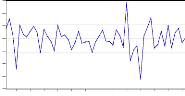
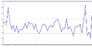
Figure 9: Residuals test
98 99 00 01 02 03 04 05 06 07 08 Rec urs ive Residuals #177; 2 S .E .
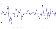
Granger ECM 10 0 -10 20 98 99 00 01 02 03 04 05 06 07 08 Figure 11: Cusum of squared test for Engle- Granger ECM
98 99 00 01 02 03 04 05 06 07 08
From the above test results the model proves its adequacy in term of coefficients and p-values. The results provide strong support for the conventional ECM model as a description of inflationary processes in Rwanda. They are consistent with the conventional theory, and with the findings of many overseas studies. They are also consistent with our understanding of the institutional structure of the domestic economy. The results suggest that about three quarters of the long-run movement in prices in Rwanda has been underpinned by import prices; about one quarter has been driven by domestic labour costs. The small coefficient on the error correction term points to protracted periods of disequilibrium for long run and drawn out adjustment processes, particularly in respect of changes to unit labour costs. In the interim, domestic demand conditions play an important role. Many indicators are using to evaluate the quality of the model proved to be used as prediction model the more used are MAPE (mean absolute percentage error), and the Inequality coefficient of THEIL, the model with small MAPE is judged sion and Theil comprised between 0 and 1 indicate r instance (see figure 13)
Figure 12: Inflation forecasting criteria Forecast: DLIPCF Actual: DLIPC Forecast sample: 1995Q1 2009Q2 Adjusted sample: 1995Q4 2009Q2 Included observations: 55
The two models seen above have the same characteristics and don't allow us to make the best forecast because the mean absolute percentage error is high in two equations above see Figure 6. Instead of using one of them we extend our understanding by apply the VECM as theoretical suggest. The main reason for estimating a VECM system of equations is because arguments call for the lag between cause and effect to be shorter than the forecast horizon. Forecast the causal variables are needed and estimating VECM will automatically provide them. We initially estimate equation in level not in first differences because it's often possible to find a group of variables that is stationary even thought the individual variable are not. Such a group is cointegrating vector, if the values of two variables tend to move together over time so that their values are always in the some ratio to each other, then the variables are cointegrated. This is the desirable long run relationship between a causal and dependent variables. The value of the causal predicts the value of the dependent variable but in particular time the prediction is not er be large. An article that should become classical 1994)49.
3.3. Forecasting inflation using VECM An error correction model contains one or more long run cointegration relationship as seen above but using the VECM will while not necessary to go back to cointegration concepts is helpful in making the connection between a VAR with variables in levels the error correction form and a VECM with variable in differences. From a theory standpoint the parameters of the system will be estimated consistently and even if the true model is in differences, hypothesis tests based on an equation in levels will have the same distribution as if the correct model had been used. 3.3.1 Why a VECM? Because any exercise in empirical macroeconomic must recognize the conclusion drawn from times series analyses of macroeconomic data, and utilize specifications that are consistent with these results. Such analyses starting with the classic study of Nelson and Plosser (1982), consistently have demonstrated that macroeconomic time series data likely include a component generated by permanent or nearly permanent shocks. Such data series are said to be integrated, difference stationary, or to contain unit roots. On the other hand, economic theories suggest that some economic variables will not drift independently of each other forever, but ultimately the difference or ratio of such variables will revert to a mean or a time trend50. Granger defined variables that are individually driven by permanent shocks (integrated), but for which there are weighted sums (linear combinations) that are mean reverting (driven only by transitory shocks), as cointegrated variables. He then demonstrated in the Granger Representation Theorem (Engle and Granger, 1987; Johansen, 1991) that variables, individually driven by permanent shocks, are 49 Murray, M. P(1994), «A drunk and her dog: An illustration of cointegration and error correction,» American Statistician, 48, 37-39. 50 Klein, L.B. and B. F. Kosobud (1961), «Some Econometrics of Growth: Great Batios of Economics», Quarterly Journal of Economics, 75:173-98.
xists a Vector Error Correction representation of the 3.3.2. Forecasting performance While the cointegrating vectors determine the steady-state behavior of the variables in the Vector Error Correction Model, the dynamic responses of each of the variables to the underlying permanent and transitory shocks are completely determined by the sample data without any restriction. Forecasting performance may be gauged in a number of different ways. Papers by Clements and Hendry (1993) and Hoffman and Rasche (1996b) employ measures of system performance, while Clements and Hendry (1993) and Christofferson and Diebold (1996) argue that conventional RMSE criterion may not capture some of the advantages of long-run information into the system. The basic conclusion of this body of literature is that incorporating cointegration may improve forecast performance, but improvement need not show up only at longer horizons as predicted originally by Engle and Yoo (1987). The advantage presumably accrues from the addition of error correction terms in VECM representations. Christofferson and Diebold (1996) contend that conventional RMSE criterion will not capture this forecast advantage at long forecast horizons simply because the importance of the error correction term diminishes with increases in the forecast horizon. For the exercise we have in mind, the relevant issue is forecast performance for a subset of the variables in our system, at various horizons, and the most relevant measure of that performance is the standard mean squared error criterion. We employ RMSFE as a criterion while recognizing that it may not capture all the advantages that the long-term information has to offer. The results for VECM are in the following table 16 The results show that the fluctuations of price level are positively related to previews price level and the mark up but negatively related to nominal GDP, exchange rate, the interest rate and the excess money supply. 51 Engle, R.F. and C.W.J. Granger (1987), «Cointegration and Error Correction: Representation, Estimation, and Testing» Econometrica, 55:251-276.
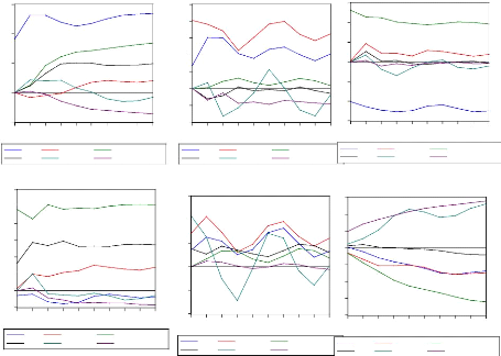
esponse of shocks on errors for all variables. For al to 2 standard deviation of errors. The temporal Horizon for response is set at 10 quarterly, this horizon represent the time needed in which the variable recover the long run level. Figure 13: Response function of variables on LIPC Response of LIPC to Cholesky Response of LMARKUP to Cholesky Response of LEXCESS_MONEY to Cholesky One S.D. Innovations One S.D. Innovations One S.D. Innovations
Response of LM2 to Cholesky LPIBC LTCUSD One S.D. Innovations Response of LPIBC to Cholesky LIPC LMARKUP LEXCESS_MONEY LM2 Response of LTCUSD to Cholesky 1 2 3 4 5 6 7 8 9 10 1 2 3 4 5 6 7 8 9 10 1 2 3 4 5 6 7 8 9 10 .08 .06 .04 .02 .00 -.02 -.04 .06 .04 .02 .00 -.02 -.04 -.06 .10 .03 .02 .01 .00 -.01 LIPC LMARKUP LEXCESS_MONEY LM2 LPIBC LTCUSD LIPC LMARKUP LEXCESS_MONE LM2 LPIBC LTCUSD 1 2 3 4 5 6 7 8 9 10 1 2 3 4 5 6 7 8 9 10 .06 .05 .04 .03 .02 .01 .00 -.01 .06 .04 .02 .00 -.02 -.04 -.01 -.02 -.03 -.04 .03 .02 .01 .00 1 2 3 4 5 6 7 8 9 10 LIPC LMARKUP LEXCESS_MONE LM2 LPIBC LTCUSD LIPC LMARKUP LEXCESS_MONEY LM2 LPIBC LTCUSD LIPC LMARKUP LEXCESS_MONEY LM2 LPIBC LTCUSD The shock is positive on LIPC generated by the negative effect of money supply, exchange rate, interest rate, and nominal GDP as seen above (seen figure 14) then the shock is negative to LIPC generated to positive effect of previews price level and mark up the whole fructuation on any variable have a significant impart on price level the figure above shows how change is made by mark up, excess money supply, money demand and GDP every period.
ition The aim of decomposition of the variance of errors of prevision is to calculate for each innovation have as contribution on the errors variance expressed in percentage, when the innovation explain the big part in variance of error we conclude that the considered economy is sensible on shock which affect the series seen the appendix 5. The decomposition of the variance show that the variance of error prevision of the LIPC is due to 80% on its own innovation, 1% of the mark up innovation,10% of excess money supply innovation, 7% of M2 innovation ,1% of GDP innovation and 2% of exchange rate innovation. The variance of error of the others variable is represented on the appendix 5 all of them show the accuracy. .3.3.2.2 Forecast results The forecast was produced using the data available through the first quarter of 1995. Table 16 provides the numeric forecasts both quarter-by-quarter and on an annual basis. The annual values for the levels of real GDP, nominal M2, and the two interest rate series are four-quarter averages. The annual values for the inflation rates and growth rates are measured on a fourth-quarter to fourth-quarter basis. Real growth for the third quarter of 2009 is forecast to be very slow, indeed to decline from the rate of 2010.1. In retrospect we know that this was a really large forecast error, since the third quarter of 2009 came in exceptionally strong. The forecast is for continued slow real growth (< 1 percent per quarter) though the end of 2010. This certainly will be an underestimate of real growth for 2009, and appears at this time (January, 2010) to be an underestimate of real growth for 2010. In addition, the forecast did not catch the large increase in long rates and the accompanying increase in the slope of the yield curve that began in the last part of the 2010:1 and continued through third quarterly. In comparison, the money supply (M2) is projected to remain essentially constant through 2009 (around 6.10 percent), not far from the actual experience. Thus the long-term rate forecast errors in 2010 are attributable to errors in the implicit short-run term structure relationship. Taken literally, the model is forecasting a reduction in the exchange rate target to around
10. Finally, the model projects no change in the o inflation rates (at roughly 2.5 percent per annum in terms of the CPI inflation rate) through the end of 2010. Hence the model is not predicting any increase in the long-run rate of inflation over this period. Table 15: Prevision results
The table15 above show the prevision of future variables and demonstrate how change will have the price level due to change of other variables here the variable are in percentage change. For example to comparing two period in 2nd quarterly of 2009 inflation was 185.30 expressed as CPI and 3rd quarterly the price level is 185.75 mean the evolution of 0.65% per/quarterly, the price level in 4th quarterly will be 186.04 mean evolution of 0.54%, the price level of 1st quarterly 2010 will be 186.38 mean evolution of 0.62% per quarterly, in the 2nd quarterly of 2010 the price level will be 186.86 mean evolution of 0.89% per period and the 3rd quarterly price level will be 187.23 mean the evolution of 0.7% per period. These fluctuations are results of demand shocks on one hand and the supply shocks on other.
model for forecasting because there are weighted sums (linear combinations) that are mean reverting (driven only by transitory shocks), as cointegrated variables and each variables is individually driven by permanent shocks, are cointegrated if and only if there exists a Vector Error Correction representation of the data series Nelson and Plosser (1982). The VECM has predicted inflation reasonably well over history and still appears to be a good forecasting model, especially in light of modifications like using adjusted, identifying policy shocks, and deriving probabilities for inflation outcomes.
The Rwanda inflation is driven in great part by the increase in money supply as it have been seen above but the excess money supply doesn't have the direct impact on price level its act through the exchange rate, and interest rate channel. These results provide useful insights into the behavior of inflation in Rwanda and the role of the National Bank of Rwanda in its determination. Inflation appears to be driven by both foreign and domestic factors in a manner consistent with conventional theoretical models and our understanding of the institutional structure of Rwanda economy. The results suggest that maintaining low inflation in coming years will depend largely on low level of interest rate, import, oil products in partner's countries and moderate growth of money supply and domestic unit labour costs. We have analyzed the inflation in two ways; first by the demand side as demand push inflation and on other hands by the supply side as cost push inflation.
monetary variables are found to be important in ar as narrow monetary aggregate is concerned, one can notice that the magnitude of its influence on consumer price inflation is quite marginal. For forecast purpose we designed ECM model first by Hendry equations is not a perfect one, secondly by Engle Granger which proven instable by forecast criteria this is because of a high number of parameters estimated, while the definability of some equations is relatively high (a low relative coefficient of determination). However, they may be applied to the forecasting of inflation because the mean square errors of the forecast conform to the selected minimum criteria (1 or 5% should be mentioned). One of the main drawbacks of the VECM model, where the VAR methodology is used, is the fact that each time additional observations appear and the model is estimated as new equation of each group may be complemented (or reduced) by different variables. However, given stable parameters, the accuracy of results is not damaged. Nevertheless, the designing of a structural VAR or multi-equation econometric model for the forecasting of the CPI should probably be considered in future. The VECM has predicted inflation reasonably well over history and still appears to be a good forecasting model, especially in light of modifications like using adjusted, identifying policy shocks, and deriving probabilities for inflation outcomes. Forecasts from the VECM can augment the information coming from other models used at the Bank. They can provide alternative views of what could happen in the economy and give some information about the «balance of risks.» Multiple models could be especially helpful to policy-makers during times of extreme uncertainty and/or structural shifts, but even in relatively stable times, advice from different models helps to balance risks about the outlook for the future. According to the accuracy of the forecast calculated by the VECM model, this model could be suggested as a tool applied by the economists-analysts in the decision making procedure.
Some caveats are in order. First, the approach in this paper has been to evaluate forecasting performance using a simulated out of sample methodology. This methodology provides a degree of protection against overfitting and detects model instability. However, because a large number of forecasts were used, some over fitting bias nonetheless remains. This suggests that some of the best-performing forecasts produced using individual economic indicators might deteriorate as one move beyond the end of our sample. That is why the model used here could be improved in the future because; - Coefficients of predictors can change over time - The number of predictors can be large - The relevant model for forecasting can potentially change over time - The variables can also change over time Second, we have considered only linear models. To the extent that the relation between inflation and some of the candidate variables is nonlinear, these results understate the forecasting improvements that might be obtained. Moreover, with few exceptions, incorporating other variables could be necessary to improve upon the short run forecasts and must be considered by National Bank agent in their future research.
Principle of forecasting; A handbook for A
2001) : Research methodology course for the es , 2nd edition , Paris, Durod Working Papers
APPENDIX 1: DATA DEFINITIONS This appendix describes the data. The list the definitions of the data and give their sources. All data are quarterly, and the sample period is 1995(1)-2009(2).
Definition: Nominal cost of all labour per unit of output. Nominal unit labour costs are defined as: salaries + payroll taxes - employment subsidies divided by gross domestic product Where salaries refers to the wages, salaries and supplements of all employee in public and private sector including volontaries wage and salary earners. The class «wage and salary earners» is only a subset of all employed people in the economy,
f-employed, employers. Unit labour costs of wage scaled up to that by adding the 5% as legal percentage of ratio payed in national social security fund( NSSF). Source: Author calculation using then NSSF data.
Definition: Automotive fuel price index or oil price index. On the monthly basis the NBR publish the quantity and the values of energy and lubricant which include piles and electrics accumulators, fuels, gaz oils, lubricating oils and others fuels products using these available data we calculate the oil price index on Layperes basis and finally adjusted on quarterly. Source: NBR, Foreign Exchange Inspection and Balance of Payments Department 5. M2 Definition: M2 is the monetary base which
include the currency in circulation plus
nd saving deposit which is published by the national s deflated using the current CPI. Source: NBR, Research department.
The GDP represent the national output is published on the year basis we estimated it using the eviews to get the quarterly data. This involves adjusting a linear interpolation of annual GDP series with weigthed percentage errors between actual quarterly data. Then the resulting was seasonally adjusted to minimize the impact of the cyclical components.
TDC IPC PERIOD M2
1995-1 1996-1 1997-1 1998-1 1999-1 2000-1 2001-1 2002-1 2003-1 2004-1 2005-1
2006-1 2007-1 2008-1 2009-1 2009-2 APPENDIX 3: RESIDUALS PROPERTIES
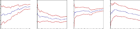
1996 1998 2000 2002 2004 2006 2008 .06 .04 .02 .00 -.02 -.04 -.06 .3 .2 .1 .0 -.1 -.2 -.3 -.4 .10 -.05 .2 .1 .0 -.1 -.2 DLPIBC Residuals DLIPC Residuals
1996 1998 2000 2002 2004 2006 2008 DLTDC Residuals DLM2 Residuals
1996 1998 2000 2002 2004 2006 2008
1996 1998 2000 2002 2004 2006 2008 DLTCUSD Residuals DLULC Residuals
1996 1998 2000 2002 2004 2006 2008 1996 1998 2000 2002 2004 2006 2008 .20 .05 -.05 .03 .02 .01 .00 -.01 -.02 -.03 Page 71
Vector Autoregression Estimates Date: 11/22/09 Time: 11:49 Sample (adjusted): 1995Q4 2009Q2 Included observations: 55 after adjustments Standard errors in ( ) & t-statistics in [ ] LIPC LIPC(-1) 1.101540 (0.26175) [ 4.20837] LIPC(-2) -0.422070 (0.27787) [-1.51896] LMARKUP(-1) -0.056816 (0.03854) [-1.47435] LMARKUP(-2) 0.013979 (0.03739) [ 0.37387] LEXCESS_MONEY(
LM2(-1) 0.111751 (0.14672) [ 0.76165] LM2(-2) 0.031747 (0.16028) [ 0.19807] LPIBC(-1) 0.089677 (0.06716) [ 1.33521] LEXCESS_
LTCUSD(-1) -0.281546 (0.14066) [-2.00166] LTCUSD(-2) 0.222899 (0.13707) [ 1.62619] C -1.676818 (1.69667) [-0.98830] R-squared 0.996371 Adj. R-squared 0.995334 Sum sq. resids 0.013769 S.E. equation 0.018106 F-statistic 960.8409 Log likelihood 150.0073 Akaike AIC -4.982082 Schwarz SC -4.507621 Mean dependent 0.043181 S.D. dependent 0.265052
[-0.47015]
Appendix 5: Variance decomposition of VECM
74863 18.69154 7.959918 0.875919 2.673639 RKUP: LEXCESS
MONEY LM2 LPIBC LTCUSD Perio d S.E. LIPC LMARKUP _
Variance Decomposition of LEXCESS_MONEY:
Variance Decomposition of LPIBC: Perio d S.E. LIPC LMARKUP LEXCESS MONEY LM2 LPIBC LTCUSD _
22762 4 0.098952 14.50754 37.38808 5 0.102642 15.49777 38.18783 6 0.116172 18.32080 38.82996 7 0.130118 20.95032 39.69009 8 0.136354 21.16591 39.71859 9 0.140460 20.28022 39.00492 10 0.143889 20.17289 40.02714
Variance Decomposition of LTCUSD: Period LEXCESS S.E. LIPC LMARKUP MONEY LM2 LPIBC LTCUSD _
Cholesky Ordering: LIPC LMARKUP LEXCESS_MONEY LM2
1.5 1.0 0.5 0.0 -0.5 -1.0 00 01 02 03 04 05 06 07 08
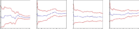
Recursive C(1) Estimates #177; 2 S.E. .05 .00 -.05 -.10 -.15 -.20 -.25 -.30 00 01 02 03 04 05 06 07 08 .2 .0 -.2 -.4 -.6 00 01 02 03 04 05 06 07 08
Recursive C(2) Estimates #177; 2 S.E. .6 .4 .2 .0 -.2 00 01 02 03 04 05 06 07 08 .25 .20 .15 .10 .05 .00 -.05 -.10 00 01 02 03 04 05 06 07 08
Recursive C(3) Estimates #177; 2 S.E. .2 -.1 -.2 -.3 00 01 02 03 04 05 06 07 08 0.4 0.0 -0.4 -0.8 -1.2 00 01 02 03 04 05 06 07 08
Recursive C(4) Estimates #177; 2 S.E. .6 .4 .2 .0 -.2 -.4 00 01 02 03 04 05 06 07 08
Recursive C(5) Estimates #177; 2 S.E.
Recursive C(6) Estimates #177; 2 S.E.
Recursive C(7) Estimates #177; 2 S.E.
Recursive C(8) Estimates #177; 2 S.E.
.8 .4 .0 -.4 -.8
Recursive C(9) Estimates #177; 2 S.E. 00 01 02 03 04 05 06 07 08 .3 .2 .1 .0 -.1 -.2
Recursive C(10) Estimates #177; 2 S.E. 00 01 02 03 04 05 06 07 08
|
| ||||||||||||||||||||||||||||||||||||||||||||||||||||||||||||||||||||||||||||||||||||||||||||||||||||||||||||||||||||||||||||||||||||||||||||||||||||||||||||||||||||||||||||||||||||||||||||||||||||||||||||||||||||||||||||||||||||||||||||||||||||||||||||||||||||||||||||||||||||||||||||||||||||||||||||||||||||||||||||||||||||||||||||||||||||||||||||||||||||||||||||||||||||||||||||||||||||||||||||||||||||||||||||||||||||||||||||||||||||||||||||||||||||||||||||||||||||||||||||||||||||||||||||||||||||||||||||||||||||||||||||||||||||||||||||||||||||||||||||||||||||||||||||||||||||||||||||||||||||||||||||||||||||||||||||||||||||||||||||||||||||||||||||||||||||||||||||||||||||||||||||||||||||||||||||||||||||||||||||||||||||||||||||||||||||||||||||||||||||||||||||||||||||||||||||||||||||||||||||||||||||||||||||||||||||||||||||||||||||||||||||||||||||||||||||||||||||||||||||||||||||||||||||||||||||||||||||||||||||||||||||||||||||||||||||||||||||||||||||||||||||||||||||||||||||||||||||||||||||||