Télédétection du manteau neigeux et modélisation de la contribution des eaux de fonte des neiges aux débits des oueds du haut atlas de Marrakech

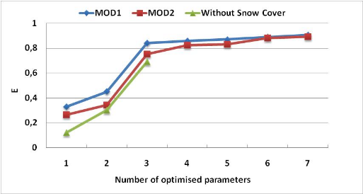
VI.5.2 Sensitivity analysis and parameters optimization

Separate model calibration is performed for the two SCA products, i.e. the one computed from SPOT VEGETATION (MOD1) and the other generated with the degree day method (MOD2). In order to perform a classical split-sample analysis, 2005 was chosen, where relatively good hydrometeorological data is available. In contrast to other years, in 2005 the measured runoff/rainfalls are consistent and they are continuously available in all sub-catchments. An automatic approach was carried out for model calibration by varying randomly each parameter value over a specified realistic searching interval ( Table ýVI ). The objective of the calibration procedure was to maximize the Nash & Sutcliffe (1970) efficiency ( Équation ýVI ) but the volume error (Dv) (i.e. mean difference between simulated and observed runoff) was also computed ( Équation ýVI Équation ýVI ).

Équation ýVI-

Équation ýVI-

Where Q_i is the measured daily streamflow, Q'_i is the modelled daily streamflow and is the average of measured streamflow over the calibration period, V_R is the measured cumulative streamflow volume and V'_R is the simulated cumulative streamflow volume.

A sensitivity analysis was carried out separately for each sub-catchment to identify the most sensitive model parameters, i.e. the parameters for which the Nash criteria is varying the most when the parameter increases from the minimum to the maximum value of the searching interval. Parameters are listed in Table ýVI in decreasing sensitivity order.

The variation of the NASH efficiency (E) when the number of optimized parameters increases has also been investigated. The adopted iterative approach consists in: i) optimizing the most sensitive parameter first and fix the other six parameters to values corresponding to the middle of the realistic ranges given in Table ýVI , plot the resulting Nash, then ii) optimize the two most sensitive parameters and fix the other five, plot the Nash and iii) repeat this operation for each parameter in decreasing sensitivity order until all seven parameters are optimized. An example for the Rheraya sub-catchment is illustrated on Figure ýVI for MOD1 and MOD2. In order to quantify the importance of the snowfall/snowmelt processes in the modelling performance, E was also computed when all precipitation falls as snow (i.e. SCA=0 for all altitudinal bands). The graphs indicate that the performance increases rapidly when the number of parameters increases from one (x) to three (x, y, Cr). The Nash function varied from 0.33 to 0.84 in MOD1, from 0.22 to 0.75 in MOD2 and from 0.12 to 0.69 in the simulation without snow cover. 0.69 is the overall Nash maximum in the later case since there are only 3 parameters in the model without the snow module. Whereas for MOD2 a fourth (Cs) and fifth parameter (a) still brings some improvement, the first guess values of the snow module parameters are sufficient for the MOD1 configuration. This means that the first guess values of a, Tf and Tc provide a reasonable estimate of the daily melting quantities for a given remotely sensed SCA. Performances in both configurations then reach a plateau when a sixth (Tc) and seventh (Tf) parameters are calibrated and show no significant gain.

Parameters		No.	Value:
			Min.	Interval	Max.
Recession coefficient, k	x	1	0.1	0.01	1
	y	2	0.01	0.01	0.1
Rainfall runoff coefficient, Cr		3	0.01	0.02	0.99
Snowmelt runoff coefficient, Cs		4	0.01	0.02	0.99
Degree-day factor, a (cm °C^-1 d^-1)		5	0.05	0.05	1
Critical temperature, Tc (°C)		6	0	0.2	6
Melt temperature, Tf (°C)		7	0	0.2	6

Table ýVI-: Parameter searching intervals for model calibration.

Figure ýVI-: Variation of the NASH efficiency «E» according to the number of optimized parameters using VEGETATION snow maps (MOD1), generated snow maps (MOD2) and when SCA is artificially kept as zero.