IV. DYNAMIC CASIMIR FORCE
To study the dynamic phenomena, the main physical quantity to
consider is the time height-field, h (r, t), where r
= (x, y) E R2 denotes the position
vector and t the time. The latter represents the time observation of
the system before it reaches its final equilibrium state. We recall that the
time height function h (r, t) solves a non-dissipative
Langevin equation (with noise) [28]
|
?h(r,t) ?t
|
= - äH0 [h]
äh (r, t) + í (r,
t) , (4.0)
|
K. El Hasnaoui et al. African Journal Of Mathematical Physics
Volume 8(2010)101-114
where > 0 is a kinetic coefficient. The latter has
the dimension : [] = L4 0T -1
0 , where L0 is some length
and T0 the time unit. Here, í (r,
t) is a Gaussian random force with mean zero and variance
?í (r,t)í
(r',t')? = 2ä2
(r - r')ä (t -
t') , (4.0)
and H0 is the static Hamiltonian (divided by
kBT), defined in Eq. (13).
The bare time correlation function, whose Fourier transform is
the dynamic structure factor, is defined by the expectation mean-value over
noise í
G(r - r',t -
t') =
?h(r,t)h(r',t')??
- ?h(r,t)??
?h(r',t')?? , t
> t' . (4.0)
The dynamic equation (28) shows that the time height function
h is a functional of noise í, and we write : h
= h [í]. Instead of solving the Langevin equation
for h [í] and then averaging over the noise
distribution P [í], the correlation and response functions can
be directly computed by means of a suitable field-theory, of action [28 -
31]
A [h, h] = J dt J
d2r { h?th +
?häâh°
h?h } , (4.0)
so that, for an arbitrary observable, O [æ], one
has 111 JJJ
|
?
?O?? = [dí] O [ö
[í]] P [í] =
|
f DhD?hOe-A[h,?h]
(4.0)
f DhD?he-A[h,h]
|
where h (r, t) is an auxiliary field,
coupled to an external field h (r, t). The correlation and
response functions can be computed replacing the static Hamiltonian H0
appearing in Eq. (13), by a new one : H0 [h, J] = H0 [h] -
f d2rJh. Consequently, for a given observable O,
we have
|
ä ?O?J äJ
(r,t)
|
J=0
|
? )
= ?h (r, t) O . (4.0)
|
108
[ ]
The notation ? . ?J means the average taken
with respect to the action A h, ?h, J associated with
the
Hamiltonian H0 [h, J]. In view of the structure of
equality (33), h is called response field. Now, if O =
h, we get the response of the order parameter field to the external
perturbation J
|
R (r - r',t -
t') =
|
?
ä ?h(r',t')?J =
(ti
(r,t)h(r',t')).
(4.0)
äJ (r, t) J=0
|
The causality implies that the response function vanishes for
t < t'. In fact, this function can be related to the
time-dependent (connected) correlation function using the
fluctuation-dissipation theorem, according to which
? )
?h (r, t) h
(r', t') = -è
(t - t') ?t ?h (r,
t) h (r',
t')?c . (4.0)
The above important formula shows that the time correlation
function C (r - r', t -
t') = ?ö (r, t) ö
(r', t')?c may be
determined by the knowledge of the response function. In particular, we show
that
(4.0)
t
L2? (t) =
(h2 (r, t))c = -2
f dt' Ch (r, t')
h (r, t')) .
8
The limit t ? -8 gives the natural value
L2? (-8) = 0, since, as assumed, the initial
state corresponds to a completely flat interface.
Consider now a membrane at temperature T that is
initially in a flat state away from thermal equilibrium. At a later time
t, the membrane possesses a certain roughness, L?
(t). Of course, the latter is time-dependent, and we are interested in
how it increases in time.
K. El Hasnaoui et al. African Journal Of Mathematical Physics
Volume 8(2010)101-114
109
We point out that the thermal fluctuations give rise to some
roughness that is characterized by the appearance of anisotropic humps.
Therefore, a segment of linear size L effectuates excursions of size
[32]
L? = BL? . (4.0)
Such a relation defines the roughness exponent
æ. Notice that L is of the order of the in-plane
correlation length, L?. From relation (20), we deduce the exponent
æ and the amplitude B. Their respective values
are : æ = 1 and B es.,
(kBT/ê)1/2.
In order to determine the growth of roughness L? in
time, the key is to consider the excess free energy (per unit area) due to the
confinement, ?F. Such an excess is related to the fact that the
confining membrane suffers a loss of entropy. Formula (27) tells us how ?F
must decay with separation. The result reads [32]
?F es., kBT/L2max es.,
kBT (B/L?)2/? , (4.0)
where Lmax represents the wavelength above
which all shape fluctuations are not accessible by the confined membrane. The
repulsive fluctuation-induced interaction leads to the disjoining pressure
|
??F
_
Ð DL?
|
es., L-(1+2/?). (4.0)
?
|
In addition, a care analysis of the Langevin equation (28) shows
that
|
?L???F ?tes., -
?L?
|
= × Ð es., L-(1+2/?) .
(4.0)
?
|
(4.0)
2 + 2æ 4
We emphasize that this scaling form agrees with Monte Carlo
predictions [32, 33]. Solving this first-order differential equation
yields [34]
1
= .
L? (t) es.,
?lt?l , è? = æ
This implies the following scaling form for the linear size
|
L (t) es.,
?iit?ii , è? =
|
1= 1
2 + 2æ 4 . (4.0)
|
Let us comment about the obtained result (39).
Firstly, as it should be, the roughness increases with time (the
exponent è? is positive definite). In addition, the exponent
è? is universal, independently on the membrane bending
rigidity constant ê. Secondly, we note that, in Eq. (39), we
have ignored some non-universal amplitude that scales as ê-1/4.
This means that the time roughness is significant only for those biomembranes
of small bending rigidity constant.
Fourthly, this time roughness can be interpreted as the
perpendicular size of holes and valleys at time t. Fifthly, the
roughness increases until a fine time, ô. The latter can be
interpreted as the time over which the system reaches its final equilibrium
state. This characteristic time then scales as
ô es., -1L1/?l
? , (4.0)
where we have ignored some non-universal amplitude that scales
as ê. Here, L? es., D is the final
roughness. Explicitly, we have
ô es., -1D4 .
(4.0)
As it should be, the final time increases with increasing film
thickness D. On the other hand, we can rewrite the behavior (39) as
|
L? (t) L?
(ô)
|
= I T I?l. (4.0)
|
K. El Hasnaoui et al. African Journal Of Mathematical Physics
Volume 8(2010)101-114
This equality means that the roughness ratio, as a function of
the reduced time, is universal.
Now, to compute the dynamic Casimir force, we start from a
formula analog to that defined in Eq. (24), that is
11(t) 1
=
kBT Ó
? ln Z? 1 ?u ? ln
Z?
?D = ?u , (4.0)
Ó ?D
with the new partition function
fZ? =
DhD?he-A[h,?h] .
(4.0)
11(t) 1
kBT 2
?u
A simple algebra taking into account the basic relation
(35a) gives
?D L2 ? (t) , (4.0)
which is very similar to the static relation defined in Eq. (25),
but with a time-dependent membrane roughness, L? (t).
Combining formulae (43) and (46) leads to the desired expression
for the time Casimir force (per unit area)
|
11(t) 11(ô)
|
( t \?'
= ,
ô
|
(4.0)
|
where 11 (ô) is the final static Casimir force,
relation (25). The force exponent, èf, is such that
æ 1
èf = 2è? =
(4.0)
1 + æ 2
= .
110
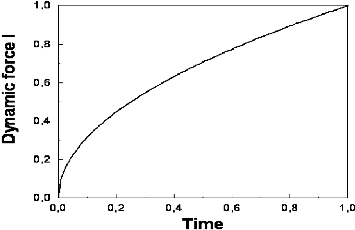
The induced force then grows with time as
t1/2 until it reaches its final value 11
(ô). At fixed time and separation D, the force
amplitude depends, of course, on ê, and decreases in this
parameter according to ê-3/2. Also, we note that the
above equality means that the force ratio as a function of the reduced time is
universal.
In Fig. 2, we draw the reduced dynamic Casimir force, 11
(t) /11 (ô), upon the renormalized time
t/ô.
K. El Hasnaoui et al. African Journal Of Mathematical Physics
Volume 8(2010)101-114
FIG. 2. Reduced dynamic Casimir force, 11 (t) /11 (r), upon the
renormalized time t/r.
Finally, consider again a membrane which is initially flat but
is now coupled to overdamped surface waves. This real situation corresponds to
a confined membrane subject to hydrodynamic interactions. The roughness now
grows as [35]
|
?L? (t) t???
|
,
|
?è? = æ
1 + 2æ
|
1
= 3 . (4.0)
|
111
Therefore, the roughness increases with time more rapidly
than that relative to biomembranes free from hydrodynamic interactions.
In this case, the dynamic Casimir force is such that
|
11h (t) 11(ôh)
|
( t )
= ôh
|
??f
|
,
|
(4.0)
|
where 11 (ôh) is the final static Casimir force,
relation (25). The new force exponent is
|
- èf = 2-è? =
2æ
1 + 2æ
|
2
= 3 . (4.0)
|
There, ôh D3 accounts for
the new time-scale over which the confined membrane reaches its final
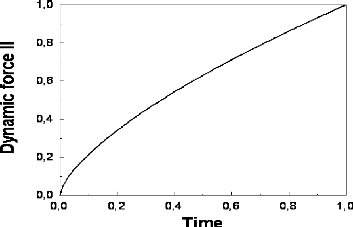
equilibrium state. Therefore, the dynamic Casimir force decays
with time as t2/3, that is more rapidly than
that where the hydrodynamic interactions are ignored, which scales rather as
t1/2. As we said before, this drastic change can
be attributed to the overdamped surface waves that develop larger and larger
humps.
We depict, in Fig. 3, the variation of the reduced dynamic
force (with hydrodynamic interactions), 11h (t) /11
(ôh), upon the renormalized time t/ôh.
K. El Hasnaoui et al. African Journal Of Mathematical Physics
Volume 8(2010)101-114
112
FIG. 3. Reduced dynamic Casimir force (with hydrodynamic
interactions), 11h (t)
/11 (r), upon the renormalized time
t/rh.
| 

