à‰pargne et bien être des ménages en RDC. Une analyse macro et microéconomique

Annexe 1 : Indicateurs macroéconomiques

année	Taux de croissance du PIB	Exportation/PIB	Importation/PIB	taux d'investissement privé	Taux d'inflation
1960		18,92	19,42	8,6	21,8
1961	-10,85	9,86	9,39	9,2	21,75
1962	21,2	7,75	7,44	9,7	17,88
1963	5,21	31,8	31,68	10,3	105,19
1964	-2,44	33,5	37,3	13	53,18
1965	1	25,92	27,23	15,2	1,32
1966	6,78	31,12	38,02	13,7	23,85
1967	-0,99	15,55	16,37	14,4	15,63
1968	4,33	14,52	15,3	15,1	17,22
1969	9,33	13,18	14,23	18,6	0,50
1970	-0,25	15,46	18,22	8,6	1,61
1971	6,01	12,14	18,54	8,9	11,27
1972	0,15	11,25	15,78	11,4	12
1973	8,14	13,44	15,88	7	11,25
1974	3,13	16,18	19,03	7,7	26,37
1975	-4,98	9,96	15,09	11,5	60,99
1976	-5,31	12,15	19,65	7,8	43,43
1977	0,76	10,33	19,67	14,8	61,06
1978	-5,35	12,35	9,2	7,7	57,38
1979	0,43	12,65	10,04	5,6	111,13
1980	2,19	16,48	16,35	3,7	47,19
1981	2,35	14,14	17,14	4,6	39,22
1982	-0,46	12,15	13,95	6,9	37,92
1983	1,41	16,24	17,29	7,2	71,90
1984	5,54	26,01	26,12	6,7	58,63
1985	0,47	27,51	25,63	7,8	13,06
1986	4,72	24,71	24,03	8,8	57,90
1987	2,68	25,98	28,86	9	84,32
1988	0,47	25,5	27,82	7,9	72,79
1989	-1,27	25,49	24,84	7,9	24,42
1990	-6,57	29,5	29,2	8,9	19,65
1991	-8,42	20,38	24,12	3,5	1141,33
1992	-10,5	16,68	17,52	4,3	2729,79
1993	-13,47	11,33	9,11	1,4	4583,08
1994	-3,9	22,63	19,89	7	9796,9
1995	0,7	28,48	23,73	5,3	370,27
1996	-1,02	30	30,31	4,6	692,96
1997	-5,62	18,75	15	2	13,76
1998	-1,62	29,79	32,89	2	134,84
1999	-4,27	23,54	17,56	2	483,72
2000	-6,9	22,38	21,37	3	511,21
2001	-2,1	18,65	20,69	5,1	313,72
2002	3,47	21,16	26,07	8	38,09
2003	5,79	26,13	33,35	9,5	12,87
2004	6,64	30,35	39,17	10	3,99
2005	6,46	34,49	42,73		21,32
2006	5,08	30,68	44,36		18,2
2007	6,26	27,17	37,94		27,6
2008	6,2	23,31	38,56		9,96
2009	2,83	9,25	20,9		53,4
2010	7,24	15,49	34,3

Source : Banque Centrale et Banque Mondiale

Annexe 2 : Liste des banques en 2010.

n°	Banques	siège social	Succursales ou agences
1	Banque commerciale du Congo (BCDC)	Kinshasa	Bukavu, Butembo, Fungurume, Goma, Kananga, Kisangani, Kinshasa, Kolwezi, Likasi, Lubumbashi, Matadi, Mbuji-Mayi.
2	banque congolaise (BC)	Kinshasa	Beni, Boma, Bukavu, Butembo, Goma, Isiro, Kisangani, Kolwezi, Lubumbashi et Uvira.
3	Afriland First Bank Congo Democratic (First Bank CD	Kinshasa	-
4	Banque Internationale pour l'afrique au Congo	Kinshasa	-
5	Citi group	Kinshasa	-
6	Stanbic Bank Congo (SBC)	Kinshasa	-
7	Access Bank (AB)	Goma/Nord Kivu	-
8	Banque Internationale de crédit (BIC)	Kinshasa	Beni, Boma, Bukavu, Butembo, Lubumbashi, Matadi, Mbanza Ngungu et Muanda.
9	Procrédit Bank Congo	Kinshasa	-
10	Raw Bank	Kinshasa	Fungurume, Kolwezi, Likasi, Lubumbashi et Matadi.
11	Trust Merchant Bank (TMB)	Lubumbashi	Kasumbalesa, Kinshasa, Kolwezi et Likasi
12	Solidaire Banque Internationale (SBI)	Kinshasa	-
13	Ecobank	Kinshasa	-
14	Mining Bank Congo (MBC)	Kinshasa	-
15	First International Bank (FI Bank)	Kinshasa	-
16	Invest Bank Congo	Kinshasa	-
17	Sofi Banque	Kinshasa	-
18	La cruche Banque	Goma/Nord Kivu	-
19	Advans Banque Congo	Kinshasa	-
20	Bank of Africa (BOA)	Kinshasa	-
21	Banque gabonnaise française	Kinshasa	-
22	United Bank Congo	Kinshasa	-

Source : Banque Centrale du Congo, Rapport annuel 2010

Annexe 3 : Indicateurs financiers

année	RM2_Ratio	Taux d'intérêt	taux d'épargne
1960	28,6521288	3,25	4,97
1961	30,4688974	3,25	5,73
1962	32,6206973	3,25	1,92
1963	26,6706217	3,25	18,65
1964	21,220908	3,25	15,21
1965	18,8523702	3,25	15,55
1966	16,7132477	3,25	1,43
1967	19,1216777	3,25	11,2
1968	19,1940568	3,25	10,46
1969	19,8980465	3,25	11,78
1970	20,2891328	3,25	12,16
1971	19,5990985	3,25	12
1972	20,485727	3,25	14,12
1973	33,9270835	3,25	14,29
1974	30,8422315	5	14,24
1975	25,8047685	5	12,69
1976	22,8502356	12	6,97
1977	20,3943499	12	12,05
1978	20,1234537	12	15,08
1979	15,1172628	12	15,35
1980	13,0043968	12	10,08
1981	11,8625004	26	7,5
1982	13,4287223	26	6,52
1983	14,4325795	29	8,27
1984	13,1296439	37	10,39
1985	12,8154905	50	14,38
1986	12,8390368	45	13,88
1987	13,0131335	55	11,28
1988	12,5419175	55	12,11
1989	16,3538816	95	14,95
1990	34,4638653	145	9,35
1991	71,4936	125	1,83
1992	147,150715	238	6,05
1993	171,815119	13	3,98
1994	162,111444	22	10,63
1995	144,041508	120	14,13
1996	124,241274	120	27,54
1997	138,309904	140	6,25
1998	151,558989	24	-1
1999	146,487957	8	9,07
2000	148,6609	14	4,46
2001	7,4	140	3,17
2002	5	24	4,05
2003	4,9	8	5,02
2004	5,4	14	3,97
2005	11,04	28	5,95
2006	24,6	40	-0,64
2007		22,5	8,78
2008		40	8,61
2009		70	17,06
2010		22

Source : Banque Mondiale et Banque Centrale du Congo

ANNEXE 3 : Questionnaire d'enquête

Dans le souci de contribuer à la recherche scientifique sur l'épargne, et de doter aux ménages d'instruments nécessaires pouvant assurer l'amélioration de leur bien-être, nous avons estimé bon de travailler sur « l'épargne et bien-être des ménages : une analyse microéconomique et macroéconomique ». Le présent questionnaire nous permettra de cerner la réalité du phénomène sous-étude. Nous vous garantissons que vos réponses resteront confidentielles et serviront unique pour des fins de la recherche.

A. Ville ou cité ?

1. Mbanza-Ngungu 2. Inkisi/kisantu

I.1. CARACTERISTIQUES DU CHEF DE MENAGES

1. Quel est l'âge du chef de ménage ?

2. Quel est votre sexe ?

1. Masculin 2. Féminin

3. Quel est votre état matrimonial ?

1. Célibataire 2. Marié(e) 3. Divorcé(e) 4. Veuf (ve)

4. Quel est votre niveau d'instruction ?

1. sans instruction 2. Primaire 3. Secondaire 4. Graduat 5. Licence

6. Post universitaire

5. Quelle est votre activité principale ?

1. employé du secteur public 2. Employé du secteur privé formel

3. Employeur du secteur informel 4. Employé du secteur informel

5. Inactif ou chômeur

6. Exercez-vous une ou plusieurs activités secondaires ?

1. oui 2. Non

7. Si oui, laquelle (lesquelles)

1. Location maison 2. Propriétaire taxi 3. Petit commerce 4. Agriculture 5. Autres

8. Si non pourquoi ?

1. le revenu est suffisamment 2. Contraintes de l'employeur 3. Autres

I.2. CARACTERISTIQUES DU MENAGE

9. Quelle est la taille du ménage 

10. Quel est le nombre d'enfants de 0 à 18 ans

11. Combien d'enfants fréquentent l'école (université)

12. Votre maison comporte combien de chambre à coucher ?

13. Combien des membres de votre ménage exercent une activité ?

14. Quel type d'activité exercent-ils ?

1. Contrat à temps plein formel 2. Contrat à temps partiel formel 3. Agriculture

4. Petit commerce 5. Autres à préciser

I.3. CONDITIONS DE VIE ET PATRIMOINE DU MENAGE

15. Votre maison est-elle pavée en ciment gris ou carreaux ?

1. oui 2. Non

16. Etes-vous raccordé en électricité ?

1. oui 2. Non

17. Avez-vous l'accès aux soins de santé ?

1. oui 2. Non

18. Disposez-vous d'un appareil de communication ?

1. oui 2. Non

19. Disposez -vous des appareils électroménagers ?

1. Oui 2. Non

20. Lequel(s)

1. Radio 2. TV 3. Parabole 4. DVD 5. Ordinateur 6. Réfrigérateur

7. Cuisinière 8. Micro-onde 9. Machine à laver 10. Fer à repasser 11. ventilateur-climatiseur 12. Réchaud

21. Avez-vous un cheptel ?

1. oui 2. non

II. REVENU DES MENAGES

22. Quel est le revenu mensuel de l'activité principale du chef des ménages ? _______

23. Quel est le revenu mensuel de l'activité secondaire du chef des ménages ? ______

24. Quel est le revenu des membres des ménages qui travaillent ? __________

28. Recevez-vous des transferts auprès des autres ménages évoluant au pays ?

1. oui 2. Non

25. Si oui, à combien pouvez vous l'estimer

1. 0$ 2. Moins de 100$ 3. 100-200$

4. 200-300$ 5. 300-400$ 6. 500 et plus

26. Qui opèrent ces transferts ?

1. les enfants 2. Les amis 3. Les autres membres de famille

27. Recevez-vous des transferts auprès des autres ménages évoluant à l'extérieur du pays ?

1. oui 2. Non

28. Qui opèrent ces transferts ?

1. les enfants 2. Les amis 3. Les autres membres de famille

III. CONSOMMATION DES MENAGES

29. Combien de fois mangez-vous le jour?

1. une fois 2. Deux fois 3. Trois fois 4. Quatre fois

30. Etes-vous locataire ou propriétaire

1. oui 2. non

31. Quelles sont les dépenses mensuelles ?

1. Alimentation _______________ 2. Logement (pour les locataire)______________

3. habillement _____________ 4. Santé___________ 5. Education _____________

6. eau et électricité____________ 7. Télécommunication____________

8. tourisme et loisir ____________ 9 autres _______________

32. Le revenu du ménage permet-il de faire face à toutes ses dépenses ?

1. oui 2. Non

33. Sinon, comment faites-vous pour les réaliser ?

1. emprunt 2. Désépargne 3. Transferts 4. Autre

34. Quel est le niveau de votre endettement _____________________

35. Quels sont vos différents créanciers ?

1. banque 2. Microcrédit 3. Amis et famille 4. Votre employeur 5. Banque Lambert

6. Autres

36. Payez-vous des intérêts sur ces emprunts ?

1. oui 2. Non

37. Si oui, quel est le taux

1. moins de 10% 2. 10 -20% 3. 20-30% 4. 30-40% 5. 40-50 6. 50% et plus

IV. EPARGNE DES MENAGES

38. Epargnez-vous en argent ?

1. Oui 2. Non

39. Si oui, dans quelle institution financière ou monétaire le faites-vous ?

1. Banque 2. Coopérative d'épargne et de crédit 3. Tontine 4. Garde fonds

40. Quel est le niveau de votre épargne ? ____________________

41. En quelle monnaie épargnez-vous ?

1. Monnaie nationale 2. Monnaie étrangère 3. Les deux

42. Epargnez-vous en nature ?

1. oui 2. Non

43. Quels sont les actifs que vous détenez ?

1. Stock marchandises 2. Cheptel 3. Maisons 4. Terres agricoles 5. Voitures

6. Autres biens durables

44. Etes - vous assuré ?

1. oui 2. Non

45. Si oui quel type d'assurance ?

1. assurance maladie 2. Assurance véhicule 3. Assurance vie 4. Assurance incendie

5. autres

46. Pourquoi épargnez-vous ?

1. Pour motif de précaution (faire face aux dépenses imprévues)

2. Accumuler du capital (fond de démarrage d'une activité)

3. Préparer la retraite

4. Acheter des biens durables (maisons, voitures, télévisions, ...)

5. Taux d'intérêt (gagner dans le futur)

47. Le revenu tiré de votre activité principale vous permet-il d'épargner ?

1. Oui 2. Non

48. Si non, comment faites-vous pour épargner ?

1. Activités secondaires 3. Autres à préciser.

2. Réception de fonds venant des amis et familles

49. Gardez-vous de l'argent chez vous au-delà des besoins immédiats ?

1 = Oui 2 = Non

50. Etes-vous membre d'une tontine ?

1. Oui 2. Non

56. Si Oui, combien cotisez-vous à la tontine par Période ? __________________

51. Avez-vous un compte d'épargne ?

1. Oui 2. Non

52. Si Oui, combien avez-vous à la caisse d'épargne ? _________________

53. Avez-vous de l'argent auprès des gardes fonds ?

1. Oui 2. Non

54. Si oui, combien avez-vous _____________________

55. Avez-vous un compte bancaire ?

1. Oui 2. Non

56. Si Oui, combien avez-vous en banque ? _______________________

57. Cotisez-vous à l'INSS ?

1. OUI 2. NON

58. Si oui, êtes-vous capable de vérifier le montant de votre épargne retraite auprès de cette institution ?

1. OUI 2. NON

59. Pouvez-vous compter sur cette épargne pour la retraite ?

1. OUI 2. NON

60. Si non, comment allez-vous en sortir ?

1. enfants 2. Epargne constituée auprès des autres institutions 3. Epargne en actifs réels 4. Autres à préciser

61. Si vous n'épargnez pas, pourquoi ne le faites-vous pas ?

1. Faiblesse de revenu

2. Faiblesse du taux d'intérêt (faible rémunération de l'épargne)

3. Manque d'information

4. Manque de confiance vis-à-vis du Secteur financier

5. Autres raisons.

Merci

ANNEXE 4 : Guide d'entretien

A. Institution micro finance ou bancaire

1. Quels sont les instruments d'épargne que vous offrez aux épargnants ?

2. Quels sont les avantages de chaque instrument ?

3. Quel est le volume de l'épargne de votre institution ?

4. Comment faites-vous pour attirer les agents économiques à épargner dans votre organisation ?

5. Quel est le dépôt minimum pour un agent qui veut ouvrir un compte d'épargne ?

6. Exigez-vous au récipiendaire d'avoir un parrain ?

7. Quelles sont les exigences d'octroi des crédits aux épargnants

8. Je peux accéder à vos bilans d'exploitation ?

9. Fixez-vous de taux d'intérêt en Francs, en dollars ?

10. Comment procédez-vous pour fixer le taux en dollar d'autant plus que la banque centrale fixe son taux uniquement en Francs ?

Merci

B. Sonas

1. Quels sont les différents types d'assurance dont vous disposez ?

2. Comment fonctionne ces instruments ?

3. Quels sont d'après vous les avantages liés à chaque instrument ?

4. Pensez vous qu'un ménage peut préparer sa retraite en comptant sur vos services ?

Merci

C. INSS

1. Comment fonctionne votre service de sécurité sociale ?

2. Comment est ce que vous indemnisez les retraités ?

3. Pensez vous qu'un ménage peut préparer sa retraite en comptant sur votre service ?

Merci

ANNEXE 5 : Outputs

5.1. Outputs des estimations macroéconomiques

5.1.1. Etude de la stationnarité

Null Hypothesis: SL has a unit root
Exogenous: Constant, Linear Trend
Lag Length: 0 (Automatic based on SIC, MAXLAG=1)
			t-Statistic	Prob.*
Augmented Dickey-Fuller test statistic			-3.196979	0.1020
Test critical values:	1% level		-4.252879
	5% level		-3.548490
	10% level		-3.207094
*MacKinnon (1996) one-sided p-values.
Augmented Dickey-Fuller Test Equation
Dependent Variable: D(SL)
Method: Least Squares
Date: 01/22/13 Time: 19:05
Sample (adjusted): 1971 2008
Included observations: 34 after adjustments
Variable	Coefficient	Std. Error	t-Statistic	Prob.
SL(-1)	-0.478534	0.149683	-3.196979	0.0032
C	10.14669	3.166232	3.204659	0.0031
@TREND(1970)	-0.021749	0.010062	-2.161556	0.0385
R-squared	0.249929	Mean dependent var		-0.009333
Adjusted R-squared	0.201538	S.D. dependent var		0.555114
S.E. of regression	0.496032	Akaike info criterion		1.519743
Sum squared resid	7.627468	Schwarz criterion		1.654422
Log likelihood	-22.83563	F-statistic		5.164719
Durbin-Watson stat	1.886513	Prob(F-statistic)		0.011590
Null Hypothesis: D(SL) has a unit root
Exogenous: Constant, Linear Trend
Lag Length: 0 (Automatic based on SIC, MAXLAG=1)
			t-Statistic	Prob.*
Augmented Dickey-Fuller test statistic			-6.059590	0.0001
Test critical values:	1% level		-4.284580
	5% level		-3.562882
	10% level		-3.215267
*MacKinnon (1996) one-sided p-values.
Augmented Dickey-Fuller Test Equation
Dependent Variable: D(SL,2)
Method: Least Squares
Date: 01/22/13 Time: 19:05
Sample (adjusted): 1972 2005
Included observations: 31 after adjustments
Variable	Coefficient	Std. Error	t-Statistic	Prob.
D(SL(-1))	-1.231326	0.203203	-6.059590	0.0000
C	0.026697	0.211398	0.126287	0.9004
@TREND(1970)	-0.000909	0.010572	-0.086025	0.9321
R-squared	0.567648	Mean dependent var		-0.008762
Adjusted R-squared	0.536765	S.D. dependent var		0.836573
S.E. of regression	0.569383	Akaike info criterion		1.803238
Sum squared resid	9.077513	Schwarz criterion		1.942011
Log likelihood	-24.95020	F-statistic		18.38100
Durbin-Watson stat	1.998934	Prob(F-statistic)		0.000008
Null Hypothesis: LOG(INT) has a unit root
Exogenous: Constant, Linear Trend
Lag Length: 0 (Automatic based on SIC, MAXLAG=1)
			t-Statistic	Prob.*
Augmented Dickey-Fuller test statistic			-2.901860	0.1733
Test critical values:	1% level		-4.219126
	5% level		-3.533083
	10% level		-3.198312
*MacKinnon (1996) one-sided p-values.
Augmented Dickey-Fuller Test Equation
Dependent Variable: D(LOG(INT))
Method: Least Squares
Date: 01/22/13 Time: 19:06
Sample (adjusted): 1971 2008
Included observations: 38 after adjustments
Variable	Coefficient	Std. Error	t-Statistic	Prob.
LOG(INT(-1))	-0.376554	0.129763	-2.901860	0.0064
C	0.988352	0.388174	2.546155	0.0154
@TREND(1970)	0.013916	0.014111	0.986178	0.3308
R-squared	0.198963	Mean dependent var		0.066059
Adjusted R-squared	0.153189	S.D. dependent var		0.900074
S.E. of regression	0.828269	Akaike info criterion		2.536699
Sum squared resid	24.01103	Schwarz criterion		2.665982
Log likelihood	-45.19728	F-statistic		4.346678
Durbin-Watson stat	1.876278	Prob(F-statistic)		0.020603
Null Hypothesis: D(LOG(INT)) has a unit root
Exogenous: Constant, Linear Trend
Lag Length: 1 (Automatic based on SIC, MAXLAG=1)
			t-Statistic	Prob.*
Augmented Dickey-Fuller test statistic			-6.706278	0.0000
Test critical values:	1% level		-4.234972
	5% level		-3.540328
	10% level		-3.202445
*MacKinnon (1996) one-sided p-values.
Augmented Dickey-Fuller Test Equation
Dependent Variable: D(LOG(INT),2)
Method: Least Squares
Date: 01/22/13 Time: 19:07
Sample (adjusted): 1973 2008
Included observations: 36 after adjustments
Variable	Coefficient	Std. Error	t-Statistic	Prob.
D(LOG(INT(-1)))	-1.589842	0.237068	-6.706278	0.0000
D(LOG(INT(-1)),2)	0.440614	0.160451	2.746093	0.0098
C	0.370823	0.322814	1.148719	0.2592
@TREND(1970)	-0.012798	0.013982	-0.915299	0.3669
R-squared	0.636145	Mean dependent var		0.015982
Adjusted R-squared	0.602034	S.D. dependent var		1.366117
S.E. of regression	0.861809	Akaike info criterion		2.644874
Sum squared resid	23.76689	Schwarz criterion		2.820820
Log likelihood	-43.60772	F-statistic		18.64905
Durbin-Watson stat	2.307929	Prob(F-statistic)		0.000000

Null Hypothesis: LOG(INF) has a unit root
Exogenous: Constant, Linear Trend
Lag Length: 0 (Automatic based on SIC, MAXLAG=1)
			t-Statistic	Prob.*
Augmented Dickey-Fuller test statistic			-2.605859	0.2800
Test critical values:	1% level		-4.219126
	5% level		-3.533083
	10% level		-3.198312
*MacKinnon (1996) one-sided p-values.
Augmented Dickey-Fuller Test Equation
Dependent Variable: D(LOG(INF))
Method: Least Squares
Date: 01/22/13 Time: 19:08
Sample (adjusted): 1971 2008
Included observations: 38 after adjustments
Variable	Coefficient	Std. Error	t-Statistic	Prob.
LOG(INF(-1))	-0.311489	0.119534	-2.605859	0.0134
C	1.551559	0.592206	2.619965	0.0129
@TREND(1970)	-0.009666	0.020291	-0.476364	0.6368
R-squared	0.191091	Mean dependent var		0.047956
Adjusted R-squared	0.144867	S.D. dependent var		1.429553
S.E. of regression	1.321956	Akaike info criterion		3.471758
Sum squared resid	61.16484	Schwarz criterion		3.601041
Log likelihood	-62.96340	F-statistic		4.134068
Durbin-Watson stat	1.953614	Prob(F-statistic)		0.024448
Null Hypothesis: D(LOG(INF)) has a unit root
Exogenous: Constant, Linear Trend
Lag Length: 0 (Automatic based on SIC, MAXLAG=1)
			t-Statistic	Prob.*
Augmented Dickey-Fuller test statistic			-6.827590	0.0000
Test critical values:	1% level		-4.226815
	5% level		-3.536601
	10% level		-3.200320
*MacKinnon (1996) one-sided p-values.
Augmented Dickey-Fuller Test Equation
Dependent Variable: D(LOG(INF),2)
Method: Least Squares
Date: 01/22/13 Time: 19:09
Sample (adjusted): 1972 2008
Included observations: 37 after adjustments
Variable	Coefficient	Std. Error	t-Statistic	Prob.
D(LOG(INF(-1)))	-1.143061	0.167418	-6.827590	0.0000
C	0.411652	0.504812	0.815456	0.4205
@TREND(1970)	-0.020200	0.022242	-0.908222	0.3702
R-squared	0.578399	Mean dependent var		-0.080139
Adjusted R-squared	0.553599	S.D. dependent var		2.134957
S.E. of regression	1.426434	Akaike info criterion		3.625837
Sum squared resid	69.18024	Schwarz criterion		3.756452
Log likelihood	-64.07798	F-statistic		23.32251
Durbin-Watson stat	1.984198	Prob(F-statistic)		0.000000
Null Hypothesis: LOG(PIBHAB) has a unit root
Exogenous: Constant, Linear Trend
Lag Length: 1 (Automatic based on SIC, MAXLAG=1)
			t-Statistic	Prob.*
Augmented Dickey-Fuller test statistic			-1.899465	0.6347
Test critical values:	1% level		-4.226815
	5% level		-3.536601
	10% level		-3.200320
*MacKinnon (1996) one-sided p-values.
Augmented Dickey-Fuller Test Equation
Dependent Variable: D(LOG(PIBHAB))
Method: Least Squares
Date: 01/22/13 Time: 19:11
Sample (adjusted): 1972 2008
Included observations: 37 after adjustments
Variable	Coefficient	Std. Error	t-Statistic	Prob.
LOG(PIBHAB(-1))	-0.087747	0.046195	-1.899465	0.0663
D(LOG(PIBHAB(-1)))	0.727242	0.121421	5.989407	0.0000
C	0.514399	0.282465	1.821105	0.0777
@TREND(1970)	-0.003480	0.002206	-1.577689	0.1242
R-squared	0.530289	Mean dependent var		-0.033505
Adjusted R-squared	0.487588	S.D. dependent var		0.055519
S.E. of regression	0.039742	Akaike info criterion		-3.510994
Sum squared resid	0.052122	Schwarz criterion		-3.336841
Log likelihood	68.95340	F-statistic		12.41864
Durbin-Watson stat	2.083356	Prob(F-statistic)		0.000013
Null Hypothesis: D(LOG(PIBHAB)) has a unit root
Exogenous: Constant, Linear Trend
Lag Length: 0 (Automatic based on SIC, MAXLAG=1)
			t-Statistic	Prob.*
Augmented Dickey-Fuller test statistic			-2.541404	0.3078
Test critical values:	1% level		-4.226815
	5% level		-3.536601
	10% level		-3.200320
*MacKinnon (1996) one-sided p-values.
Augmented Dickey-Fuller Test Equation
Dependent Variable: D(LOG(PIBHAB),2)
Method: Least Squares
Date: 01/22/13 Time: 19:11
Sample (adjusted): 1972 2008
Included observations: 37 after adjustments
Variable	Coefficient	Std. Error	t-Statistic	Prob.
D(LOG(PIBHAB(-1)))	-0.314826	0.123879	-2.541404	0.0158
C	-0.021435	0.014953	-1.433481	0.1609
@TREND(1970)	0.000545	0.000635	0.858860	0.3964
R-squared	0.175442	Mean dependent var		2.96E-05
Adjusted R-squared	0.126938	S.D. dependent var		0.044135
S.E. of regression	0.041238	Akaike info criterion		-3.461290
Sum squared resid	0.057821	Schwarz criterion		-3.330675
Log likelihood	67.03387	F-statistic		3.617104
Durbin-Watson stat	1.949153	Prob(F-statistic)		0.037650

Null Hypothesis: D(LOG(PIBHAB),2) has a unit root
Exogenous: Constant, Linear Trend
Lag Length: 0 (Automatic based on SIC, MAXLAG=1)
			t-Statistic	Prob.*
Augmented Dickey-Fuller test statistic			-6.787861	0.0000
Test critical values:	1% level		-4.234972
	5% level		-3.540328
	10% level		-3.202445
*MacKinnon (1996) one-sided p-values.
Augmented Dickey-Fuller Test Equation
Dependent Variable: D(LOG(PIBHAB),3)
Method: Least Squares
Date: 01/22/13 Time: 19:12
Sample (adjusted): 1973 2008
Included observations: 36 after adjustments
Variable	Coefficient	Std. Error	t-Statistic	Prob.
D(LOG(PIBHAB(-1)),2)	-1.148683	0.169226	-6.787861	0.0000
C	-0.007203	0.016487	-0.436899	0.6650
@TREND(1970)	0.000430	0.000719	0.597555	0.5542
R-squared	0.583452	Mean dependent var		0.001538
Adjusted R-squared	0.558207	S.D. dependent var		0.066716
S.E. of regression	0.044345	Akaike info criterion		-3.313987
Sum squared resid	0.064893	Schwarz criterion		-3.182027
Log likelihood	62.65176	F-statistic		23.11128
Durbin-Watson stat	1.851318	Prob(F-statistic)		0.000001

Null Hypothesis: LOG(ESPER) has a unit root
Exogenous: Constant, Linear Trend
Lag Length: 1 (Automatic based on SIC, MAXLAG=1)
			t-Statistic	Prob.*
Augmented Dickey-Fuller test statistic			-4.597210	0.0039
Test critical values:	1% level		-4.226815
	5% level		-3.536601
	10% level		-3.200320
*MacKinnon (1996) one-sided p-values.
Augmented Dickey-Fuller Test Equation
Dependent Variable: D(LOG(ESPER))
Method: Least Squares
Date: 01/22/13 Time: 19:13
Sample (adjusted): 1972 2008
Included observations: 37 after adjustments
Variable	Coefficient	Std. Error	t-Statistic	Prob.
LOG(ESPER(-1))	-0.054854	0.011932	-4.597210	0.0001
D(LOG(ESPER(-1)))	0.912898	0.049883	18.30076	0.0000
C	0.209272	0.045540	4.595392	0.0001
@TREND(1970)	7.18E-05	2.68E-05	2.679967	0.0114
R-squared	0.927574	Mean dependent var		0.002123
Adjusted R-squared	0.920989	S.D. dependent var		0.004805
S.E. of regression	0.001351	Akaike info criterion		-10.27458
Sum squared resid	6.02E-05	Schwarz criterion		-10.10042
Log likelihood	194.0797	F-statistic		140.8784
Durbin-Watson stat	0.283296	Prob(F-statistic)		0.000000

Null Hypothesis: BACO has a unit root
Exogenous: Constant, Linear Trend
Lag Length: 0 (Automatic based on SIC, MAXLAG=1)
			t-Statistic	Prob.*
Augmented Dickey-Fuller test statistic			-6.309767	0.0000
Test critical values:	1% level		-4.226815
	5% level		-3.536601
	10% level		-3.200320
*MacKinnon (1996) one-sided p-values.
Augmented Dickey-Fuller Test Equation
Dependent Variable: D(BACO)
Method: Least Squares
Date: 01/22/13 Time: 19:14
Sample (adjusted): 1972 2008
Included observations: 37 after adjustments
Variable	Coefficient	Std. Error	t-Statistic	Prob.
BACO(-1)	-1.072203	0.169928	-6.309767	0.0000
C	-3.308370	1.944585	-1.701325	0.0980
@TREND(1970)	0.040873	0.083728	0.488166	0.6286
R-squared	0.540200	Mean dependent var		-0.027002
Adjusted R-squared	0.513153	S.D. dependent var		7.791891
S.E. of regression	5.436749	Akaike info criterion		6.301844
Sum squared resid	1004.980	Schwarz criterion		6.432459
Log likelihood	-113.5841	F-statistic		19.97257
Durbin-Watson stat	2.011207	Prob(F-statistic)		0.000002

Null Hypothesis: LOG(CREDIT) has a unit root
Exogenous: Constant, Linear Trend
Lag Length: 0 (Automatic based on SIC, MAXLAG=1)
			t-Statistic	Prob.*
Augmented Dickey-Fuller test statistic			-4.049968	0.0152
Test critical values:	1% level		-4.219126
	5% level		-3.533083
	10% level		-3.198312
*MacKinnon (1996) one-sided p-values.
Augmented Dickey-Fuller Test Equation
Dependent Variable: D(LOG(CREDIT))
Method: Least Squares
Date: 01/22/13 Time: 19:14
Sample (adjusted): 1971 2008
Included observations: 38 after adjustments
Variable	Coefficient	Std. Error	t-Statistic	Prob.
LOG(CREDIT(-1))	-0.646091	0.159530	-4.049968	0.0003
C	1.838332	0.544199	3.378047	0.0018
@TREND(1970)	-0.031770	0.015575	-2.039826	0.0490
R-squared	0.319156	Mean dependent var		0.011874
Adjusted R-squared	0.280251	S.D. dependent var		1.061582
S.E. of regression	0.900625	Akaike info criterion		2.704202
Sum squared resid	28.38942	Schwarz criterion		2.833485
Log likelihood	-48.37984	F-statistic		8.203401
Durbin-Watson stat	2.182835	Prob(F-statistic)		0.001198

Null Hypothesis: D(LOG(CREDIT)) has a unit root
Exogenous: Constant, Linear Trend
Lag Length: 0 (Automatic based on SIC, MAXLAG=1)
			t-Statistic	Prob.*
Augmented Dickey-Fuller test statistic			-10.23328	0.0000
Test critical values:	1% level		-4.226815
	5% level		-3.536601
	10% level		-3.200320
*MacKinnon (1996) one-sided p-values.
Augmented Dickey-Fuller Test Equation
Dependent Variable: D(LOG(CREDIT),2)
Method: Least Squares
Date: 01/22/13 Time: 19:15
Sample (adjusted): 1972 2008
Included observations: 37 after adjustments
Variable	Coefficient	Std. Error	t-Statistic	Prob.
D(LOG(CREDIT(-1)))	-1.512583	0.147810	-10.23328	0.0000
C	-0.011530	0.332161	-0.034713	0.9725
@TREND(1970)	0.000945	0.014651	0.064465	0.9490
R-squared	0.754969	Mean dependent var		0.009732
Adjusted R-squared	0.740556	S.D. dependent var		1.867989
S.E. of regression	0.951473	Akaike info criterion		2.815994
Sum squared resid	30.78023	Schwarz criterion		2.946609
Log likelihood	-49.09589	F-statistic		52.37903
Durbin-Watson stat	2.021742	Prob(F-statistic)		0.000000

5.1.2. Test de cointégration de Johansen

Date: 01/22/13 Time: 19:19
Sample: 1970 2008
Included observations: 30
Series: SL LOG(INT) LOG(INF) LOG(PIBHAB) LOG(ESPER) BACO LOG(CREDIT)
Lags interval: 1 to 1
Selected (0.05 level*) Number of Cointegrating Relations by Model
Data Trend:	None	None	Linear	Linear	Quadratic
Test Type	No Intercept	Intercept	Intercept	Intercept	Intercept
	No Trend	No Trend	No Trend	Trend	Trend
Trace	5	4	3	5	4
Max-Eig	3	3	2	2	2
*Critical values based on MacKinnon-Haug-Michelis (1999)
Information Criteria by Rank and Model
Data Trend:	None	None	Linear	Linear	Quadratic
Rank or	No Intercept	Intercept	Intercept	Intercept	Intercept
No. of CEs	No Trend	No Trend	No Trend	Trend	Trend
	Log Likelihood by Rank (rows) and Model (columns)
0	2.253491	2.253491	13.62406	13.62406	20.93141
1	28.70612	35.99960	43.69675	51.16769	58.37436
2	52.10709	62.35695	70.03821	77.79694	82.79531
3	70.53452	80.79510	86.07789	94.00155	98.85067
4	80.39123	93.95339	99.19375	107.4405	111.8416
5	88.42999	102.0189	105.1095	120.3129	123.9886
6	92.23725	107.4158	109.2085	125.9649	127.8417
7	93.75920	109.2397	109.2397	129.1647	129.1647
	Akaike Information Criteria by Rank (rows) and Model (columns)
0	3.116434	3.116434	2.825063	2.825063	2.804573
1	2.286258	1.866693	1.753550	1.322154	1.241709
2	1.659527	1.109536	0.930786	0.546871	0.546979
3	1.364365	0.880327	0.794807	0.466563	0.409956*
4	1.640585	1.003107	0.853750	0.570633	0.477225
5	2.038001	1.465409	1.392700	0.712476	0.600761
6	2.717517	2.105612	2.052768	1.335674	1.277219
7	3.549387	2.984019	2.984019	2.122352	2.122352
	Schwarz Criteria by Rank (rows) and Model (columns)
0	5.405056	5.405056	5.440631	5.440631	5.747087
1	5.228773	4.855914	5.023011	4.638321	4.838116
2	5.255934	4.799356	4.854138	4.563637*	4.797278
3	5.614664	5.270745	5.372052	5.183928	5.314147
4	6.544776	6.094124	6.084887	5.988597	6.035308
5	7.596084	7.257025	7.277729	6.831038	6.812736
6	8.929492	8.597826	8.591689	8.154835	8.143087
7	10.41525	10.17683	10.17683	9.642111	9.642111

5.1.3. Estimation 1 et Tests

Dependent Variable: D(LOG(S))
Method: Least Squares
Date: 01/22/13 Time: 19:34
Sample (adjusted): 1972 2008
Included observations: 33 after adjustments
Variable	Coefficient	Std. Error	t-Statistic	Prob.
C	-4.603817	24.78515	-0.185749	0.8546
D(LOG(INT))	0.020781	0.123451	0.168331	0.8681
D(LOG(INF))	-0.100340	0.079649	-1.259777	0.2230
D(D(LOG(PIBHAB)))	1.566020	2.101269	0.745273	0.4652
LOG(ESPER)	-46.78102	27.31560	-1.712612	0.1031
D(LOG(CREDIT))	0.022022	0.141890	0.155204	0.8783
BACO	0.026483	0.016840	1.572635	0.1323
LOG(S(-1))	-0.670678	0.213174	-3.146153	0.0053
LOG(INT(-1))	-0.065266	0.150741	-0.432969	0.6699
LOG(INF(-1))	-0.004422	0.080215	-0.055130	0.9566
LOG(PIBHAB(-1))	0.811569	0.376967	2.152891	0.0444
LOG(ESPER(-1))	47.41514	26.60020	1.782511	0.0907
LOG(CREDIT(-1))	-0.142402	0.183225	-0.777197	0.4466
BACO(-1)	-0.000700	0.018230	-0.038407	0.9698
R-squared	0.610911	Mean dependent var		-0.033135
Adjusted R-squared	0.344692	S.D. dependent var		0.570835
S.E. of regression	0.462097	Akaike info criterion		1.590334
Sum squared resid	4.057146	Schwarz criterion		2.225216
Log likelihood	-12.24051	F-statistic		2.294768
Durbin-Watson stat	2.549007	Prob(F-statistic)		0.048716

White Heteroskedasticity Test:
F-statistic	0.895278	Probability		0.612988
Obs*R-squared	24.04680	Probability		0.458924
Test Equation:
Dependent Variable: RESID^2
Method: Least Squares
Date: 01/22/13 Time: 19:45
Sample: 1972 2008
Included observations: 33
Variable	Coefficient	Std. Error	t-Statistic	Prob.
C	-6.127875	52.99098	-0.115640	0.9108
D(LOG(INT))	0.038730	0.097877	0.395696	0.7027
(D(LOG(INT)))^2	0.017461	0.171505	0.101808	0.9214
D(LOG(INF))	0.072118	0.065169	1.106620	0.3006
(D(LOG(INF)))^2	0.024516	0.052850	0.463884	0.6551
D(D(LOG(PIBHAB)))	0.137700	1.891907	0.072784	0.9438
(D(D(LOG(PIBHAB))))^2	3.067671	36.05643	0.085080	0.9343
LOG(ESPER)	-25.56550	62.19001	-0.411087	0.6918
D(LOG(CREDIT))	0.008262	0.232878	0.035479	0.9726
(D(LOG(CREDIT)))^2	0.002671	0.074436	0.035886	0.9723
BACO	0.012726	0.068172	0.186675	0.8566
BACO^2	0.000778	0.002872	0.270970	0.7933
LOG(S(-1))	0.230129	1.423713	0.161640	0.8756
(LOG(S(-1)))^2	-0.066239	0.313216	-0.211479	0.8378
LOG(INT(-1))	-0.314282	0.476655	-0.659350	0.5282
(LOG(INT(-1)))^2	0.038418	0.088345	0.434858	0.6752
LOG(INF(-1))	0.471936	0.512433	0.920971	0.3840
(LOG(INF(-1)))^2	-0.046084	0.069100	-0.666907	0.5236
LOG(PIBHAB(-1))	4.285470	23.34782	0.183549	0.8589
(LOG(PIBHAB(-1)))^2	-0.425760	2.264645	-0.188003	0.8556
LOG(ESPER(-1))	24.28589	56.99455	0.426109	0.6813
LOG(CREDIT(-1))	0.011465	0.296375	0.038684	0.9701
(LOG(CREDIT(-1)))^2	-0.029006	0.072319	-0.401078	0.6989
BACO(-1)	0.044791	0.058626	0.764004	0.4668
BACO(-1)^2	0.002218	0.002847	0.779125	0.4583
R-squared	0.728691	Mean dependent var		0.122944
Adjusted R-squared	-0.085236	S.D. dependent var		0.187108
S.E. of regression	0.194919	Akaike info criterion		-0.334382
Sum squared resid	0.303947	Schwarz criterion		0.799336
Log likelihood	30.51730	F-statistic		0.895278
Durbin-Watson stat	2.343029	Prob(F-statistic)		0.612988

ARCH Test:
F-statistic	0.283841	Probability		0.836504
Obs*R-squared	0.968845	Probability		0.808790
Test Equation:
Dependent Variable: RESID^2
Method: Least Squares
Date: 01/22/13 Time: 19:47
Sample (adjusted): 1975 2005
Included observations: 26 after adjustments
Variable	Coefficient	Std. Error	t-Statistic	Prob.
C	0.179017	0.070772	2.529482	0.0191
RESID^2(-1)	-0.190936	0.210478	-0.907158	0.3742
RESID^2(-2)	-0.089396	0.270000	-0.331097	0.7437
RESID^2(-3)	-0.025308	0.264380	-0.095726	0.9246
R-squared	0.037263	Mean dependent var		0.140561
Adjusted R-squared	-0.094019	S.D. dependent var		0.205379
S.E. of regression	0.214817	Akaike info criterion		-0.097423
Sum squared resid	1.015219	Schwarz criterion		0.096130
Log likelihood	5.266502	F-statistic		0.283841
Durbin-Watson stat	2.121181	Prob(F-statistic)		0.836504

Breusch-Godfrey Serial Correlation LM Test:
F-statistic	2.873186	Probability		0.084152
Obs*R-squared	8.336725	Probability		0.015478
Test Equation:
Dependent Variable: RESID
Method: Least Squares
Date: 01/22/13 Time: 19:49
Presample and interior missing value lagged residuals set to zero.
Variable	Coefficient	Std. Error	t-Statistic	Prob.
C	-27.98730	26.60616	-1.051910	0.3076
D(LOG(INT))	-0.105177	0.122781	-0.856616	0.4036
D(LOG(INF))	-0.021824	0.075233	-0.290089	0.7753
D(D(LOG(PIBHAB)))	0.345576	2.118687	0.163109	0.8724
LOG(ESPER)	32.05457	29.99140	1.068792	0.3001
D(LOG(CREDIT))	0.065086	0.134984	0.482177	0.6358
BACO	-0.006660	0.015933	-0.418010	0.6812
LOG(S(-1))	0.753974	0.413327	1.824159	0.0858
LOG(INT(-1))	-0.115614	0.146140	-0.791116	0.4398
LOG(INF(-1))	0.089285	0.082405	1.083491	0.2937
LOG(PIBHAB(-1))	-0.253867	0.360915	-0.703399	0.4913
LOG(ESPER(-1))	-24.87958	27.62221	-0.900709	0.3803
LOG(CREDIT(-1))	-0.026067	0.172316	-0.151276	0.8815
BACO(-1)	-0.025215	0.019864	-1.269381	0.2214
RESID(-1)	-1.151359	0.525222	-2.192138	0.0426
RESID(-2)	-0.182754	0.387230	-0.471953	0.6430
R-squared	0.252628	Mean dependent var		6.41E-15
Adjusted R-squared	-0.406818	S.D. dependent var		0.356070
S.E. of regression	0.422332	Akaike info criterion		1.420354
Sum squared resid	3.032197	Schwarz criterion		2.145933
Log likelihood	-7.435841	F-statistic		0.383091
Durbin-Watson stat	2.047113	Prob(F-statistic)		0.965919

5.1.4. Estimation 2 et ses tests

Dependent Variable: D(LOG(S))
Method: Least Squares
Date: 01/23/13 Time: 08:55
Sample (adjusted): 1972 2008
Included observations: 33 after adjustments
Variable	Coefficient	Std. Error	t-Statistic	Prob.
C	-16.26648	16.87477	-0.963953	0.3494
D(LOG(INT))	0.065223	0.076182	0.856154	0.4046
D(LOG(INF))	-0.059519	0.065407	-0.909972	0.3763
D(D(LOG(PIBHAB)))	1.596551	1.243462	1.283956	0.2174
LOG(ESPER)	-40.87276	16.42224	-2.488866	0.0242
D(LOG(CREDIT))	-0.101158	0.087150	-1.160741	0.2628
BACO	0.015025	0.010439	1.439344	0.1693
LOG(S(-1))	-0.823563	0.133600	-6.164382	0.0000
LOG(INT(-1))	-0.067047	0.106872	-0.627362	0.5393
LOG(INF(-1))	-0.050951	0.048251	-1.055940	0.3067
LOG(PIBHAB(-1))	0.963237	0.227446	4.235014	0.0006
LOG(ESPER(-1))	44.45694	15.66119	2.838669	0.0119
LOG(CREDIT(-1))	-0.101920	0.108825	-0.936544	0.3629
BACO(-1)	0.010490	0.011130	0.942459	0.3600
D76	-0.731111	0.294378	-2.483577	0.0245
D91	-1.349178	0.456320	-2.956646	0.0093
D96	1.451955	0.428657	3.387221	0.0038
R-squared	0.888221	Mean dependent var		-0.033135
Adjusted R-squared	0.776441	S.D. dependent var		0.570835
S.E. of regression	0.269902	Akaike info criterion		0.524872
Sum squared resid	1.165557	Schwarz criterion		1.295800
Log likelihood	8.339616	F-statistic		7.946185
Durbin-Watson stat	1.913479	Prob(F-statistic)		0.000076

Dependent Variable: D(LOG(S))
Method: Least Squares
Date: 01/23/13 Time: 08:55
Sample (adjusted): 1972 2008
Included observations: 33 after adjustments
Variable	Coefficient	Std. Error	t-Statistic	Prob.
C	-16.26648	16.87477	-0.963953	0.3494
D(LOG(INT))	0.065223	0.076182	0.856154	0.4046
D(LOG(INF))	-0.059519	0.065407	-0.909972	0.3763
D(D(LOG(PIBHAB)))	1.596551	1.243462	1.283956	0.2174
LOG(ESPER)	-40.87276	16.42224	-2.488866	0.0242
D(LOG(CREDIT))	-0.101158	0.087150	-1.160741	0.2628
BACO	0.015025	0.010439	1.439344	0.1693
LOG(S(-1))	-0.823563	0.133600	-6.164382	0.0000
LOG(INT(-1))	-0.067047	0.106872	-0.627362	0.5393
LOG(INF(-1))	-0.050951	0.048251	-1.055940	0.3067
LOG(PIBHAB(-1))	0.963237	0.227446	4.235014	0.0006
LOG(ESPER(-1))	44.45694	15.66119	2.838669	0.0119
LOG(CREDIT(-1))	-0.101920	0.108825	-0.936544	0.3629
BACO(-1)	0.010490	0.011130	0.942459	0.3600
D76	-0.731111	0.294378	-2.483577	0.0245
D91	-1.349178	0.456320	-2.956646	0.0093
D96	1.451955	0.428657	3.387221	0.0038
R-squared	0.888221	Mean dependent var		-0.033135
Adjusted R-squared	0.776441	S.D. dependent var		0.570835
S.E. of regression	0.269902	Akaike info criterion		0.524872
Sum squared resid	1.165557	Schwarz criterion		1.295800
Log likelihood	8.339616	F-statistic		7.946185
Durbin-Watson stat	1.913479	Prob(F-statistic)		0.000076

LE MODELE EST BIEN SPECIFIE CAR LES DEUX PROBABILITES SONT SUPERIEURES A 5%

Ramsey RESET Test:
F-statistic	0.739210	Probability		0.495234
Log likelihood ratio	3.312851	Probability		0.190820
Test Equation:
Dependent Variable: D(LOG(S))
Method: Least Squares
Date: 01/23/13 Time: 08:56
Sample: 1972 2008
Included observations: 33
Variable	Coefficient	Std. Error	t-Statistic	Prob.
C	-4.301384	24.11580	-0.178364	0.8610
D(LOG(INT))	0.045547	0.091452	0.498038	0.6262
D(LOG(INF))	-0.073862	0.067570	-1.093118	0.2928
D(D(LOG(PIBHAB)))	1.748350	1.273200	1.373193	0.1913
LOG(ESPER)	-39.41379	18.27184	-2.157078	0.0489
D(LOG(CREDIT))	-0.091965	0.089030	-1.032973	0.3191
BACO	0.009160	0.012040	0.760777	0.4594
LOG(S(-1))	-0.579302	0.253153	-2.288347	0.0382
LOG(INT(-1))	-0.018575	0.129704	-0.143208	0.8882
LOG(INF(-1))	-0.071936	0.054831	-1.311972	0.2106
LOG(PIBHAB(-1))	0.708191	0.332870	2.127529	0.0516
LOG(ESPER(-1))	40.06756	16.78287	2.387408	0.0316
LOG(CREDIT(-1))	-0.095261	0.125793	-0.757282	0.4614
BACO(-1)	0.009852	0.011552	0.852849	0.4081
D76	-0.650682	0.309249	-2.104070	0.0539
D91	-0.261274	1.043428	-0.250400	0.8059
D96	1.046165	0.549239	1.904754	0.0776
FITTED^2	0.085695	0.253158	0.338504	0.7400
FITTED^3	0.310602	0.258845	1.199957	0.2501
R-squared	0.898897	Mean dependent var		-0.033135
Adjusted R-squared	0.768908	S.D. dependent var		0.570835
S.E. of regression	0.274412	Akaike info criterion		0.545694
Sum squared resid	1.054229	Schwarz criterion		1.407320
Log likelihood	9.996041	F-statistic		6.915156
Durbin-Watson stat	2.096843	Prob(F-statistic)		0.000333

LA COURBE DE COUPE LE CORRIDOR : MCE EST STRUCTURELLEMENT STABLE

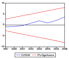
LE MODELE A CORRECTION D'ERREUR EST PONCTUELLEMENT STABLE

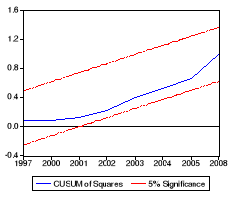
IL Y A ABSENCE D'AUTOCORRELATION

Breusch-Godfrey Serial Correlation LM Test:
F-statistic	0.764679	Probability		0.483974
Obs*R-squared	3.249898	Probability		0.196922
Test Equation:
Dependent Variable: RESID
Method: Least Squares
Date: 01/23/13 Time: 09:06
Presample and interior missing value lagged residuals set to zero.
Variable	Coefficient	Std. Error	t-Statistic	Prob.
C	-3.028769	17.47902	-0.173280	0.8649
D(LOG(INT))	-0.008335	0.079300	-0.105102	0.9178
D(LOG(INF))	0.019957	0.068459	0.291522	0.7749
D(D(LOG(PIBHAB)))	0.205258	1.301543	0.157704	0.8769
LOG(ESPER)	4.613400	17.76323	0.259716	0.7989
D(LOG(CREDIT))	0.009480	0.092360	0.102639	0.9197
BACO	-0.003672	0.011546	-0.317997	0.7552
LOG(S(-1))	0.049871	0.163473	0.305070	0.7648
LOG(INT(-1))	-0.012932	0.109218	-0.118405	0.9074
LOG(INF(-1))	0.001968	0.051565	0.038161	0.9701
LOG(PIBHAB(-1))	-0.075413	0.240476	-0.313600	0.7584
LOG(ESPER(-1))	-3.754328	16.73424	-0.224350	0.8257
LOG(CREDIT(-1))	0.023002	0.112453	0.204547	0.8409
BACO(-1)	0.003884	0.011959	0.324738	0.7502
D76	-0.011406	0.299557	-0.038075	0.9702
D91	-0.081732	0.468175	-0.174576	0.8639
D96	0.059899	0.438990	0.136448	0.8934
RESID(-1)	0.001937	0.362735	0.005340	0.9958
RESID(-2)	-0.462508	0.374205	-1.235973	0.2368
R-squared	0.098482	Mean dependent var		4.79E-15
Adjusted R-squared	-1.060613	S.D. dependent var		0.190850
S.E. of regression	0.273962	Akaike info criterion		0.542409
Sum squared resid	1.050771	Schwarz criterion		1.404034
Log likelihood	10.05025	F-statistic		0.084964
Durbin-Watson stat	1.855358	Prob(F-statistic)		0.999997

LES ERREURS SONT HOMOSCEDASTIQUES

ARCH Test:
F-statistic	0.096168	Probability		0.758774
Obs*R-squared	0.102684	Probability		0.748632
Test Equation:
Dependent Variable: RESID^2
Method: Least Squares
Date: 01/23/13 Time: 09:08
Sample (adjusted): 1973 2005
Included observations: 30 after adjustments
Variable	Coefficient	Std. Error	t-Statistic	Prob.
C	0.032912	0.011371	2.894314	0.0073
RESID^2(-1)	0.058132	0.187456	0.310110	0.7588
R-squared	0.003423	Mean dependent var		0.034909
Adjusted R-squared	-0.032169	S.D. dependent var		0.050525
S.E. of regression	0.051332	Akaike info criterion		-3.036676
Sum squared resid	0.073778	Schwarz criterion		-2.943263
Log likelihood	47.55014	F-statistic		0.096168
Durbin-Watson stat	2.025974	Prob(F-statistic)		0.758774

White Heteroskedasticity Test:
F-statistic	1.084570	Probability		0.518081
Obs*R-squared	28.18717	Probability		0.401372
Test Equation:
Dependent Variable: RESID^2
Method: Least Squares
Date: 01/23/13 Time: 09:09
Sample: 1972 2008
Included observations: 33
Variable	Coefficient	Std. Error	t-Statistic	Prob.
C	14.18080	16.57232	0.855692	0.4313
D(LOG(INT))	-0.016493	0.026703	-0.617637	0.5639
(D(LOG(INT)))^2	0.042670	0.054012	0.790011	0.4653
D(LOG(INF))	-0.112846	0.042940	-2.627993	0.0466
(D(LOG(INF)))^2	-0.037482	0.020857	-1.797069	0.1323
D(D(LOG(PIBHAB)))	-0.821679	0.523658	-1.569114	0.1774
(D(D(LOG(PIBHAB))))^2	-2.709021	11.09420	-0.244183	0.8168
LOG(ESPER)	1.024734	22.17876	0.046203	0.9649
D(LOG(CREDIT))	-0.081349	0.066147	-1.229835	0.2735
(D(LOG(CREDIT)))^2	-0.030524	0.020305	-1.503272	0.1931
BACO	-0.021916	0.020873	-1.049983	0.3418
BACO^2	-0.001121	0.000886	-1.264965	0.2616
LOG(S(-1))	-0.074620	0.484521	-0.154007	0.8836
(LOG(S(-1)))^2	0.023800	0.111897	0.212696	0.8400
LOG(INT(-1))	0.424386	0.285306	1.487479	0.1970
(LOG(INT(-1)))^2	-0.065007	0.046031	-1.412235	0.2170
LOG(INF(-1))	-0.336922	0.199381	-1.689842	0.1519
(LOG(INF(-1)))^2	0.026757	0.023311	1.147835	0.3030
LOG(PIBHAB(-1))	-4.267609	7.779023	-0.548605	0.6069
(LOG(PIBHAB(-1)))^2	0.411146	0.758052	0.542371	0.6109
LOG(ESPER(-1))	-1.817260	19.42609	-0.093547	0.9291
LOG(CREDIT(-1))	-0.054650	0.075647	-0.722431	0.5024
(LOG(CREDIT(-1)))^2	0.052469	0.028868	1.817535	0.1288
BACO(-1)	-0.053652	0.022097	-2.428031	0.0595
BACO(-1)^2	-0.002436	0.001026	-2.373570	0.0637
D76	-0.016266	0.078299	-0.207735	0.8436
D91	0.800066	0.427002	1.873681	0.1198
D96	0.882074	0.335344	2.630354	0.0465
R-squared	0.854157	Mean dependent var		0.035320
Adjusted R-squared	0.066603	S.D. dependent var		0.050804
S.E. of regression	0.049083	Akaike info criterion		-3.380727
Sum squared resid	0.012045	Schwarz criterion		-2.110963
Log likelihood	83.78199	F-statistic		1.084570
Durbin-Watson stat	2.735793	Prob(F-statistic)		0.518081

LES ERREURS SONT NORMALEMENT DISTRIBUEES

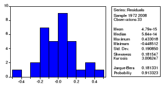
5.2. Outputs estimation micro : Relation entre revenu et bien-être

5.2.1. Output modèle Probit

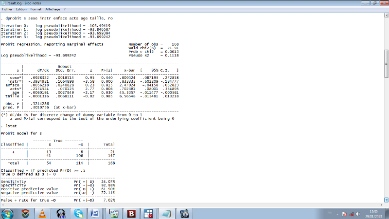
Tableau de Prédiction du modèle Probit

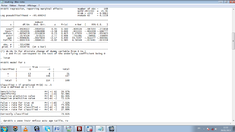
5.2.2. Différence simple de moyenne du revenu

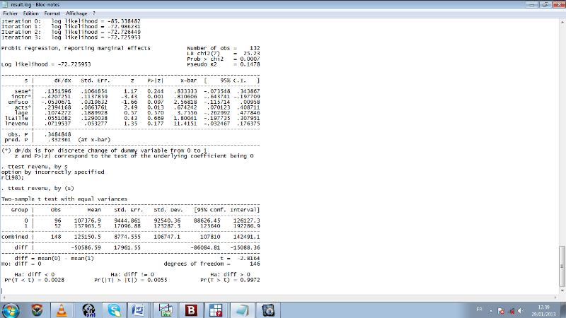
5.2.3. Outputs estimation revenu sur le revenu et quelques variables caractéristiques du ménage

Dependent Variable: LOG(REV)
Method: Least Squares
Date: 01/27/13 Time: 14:50
Sample (adjusted): 2 200
Included observations: 95 after adjustments
Variable	Coefficient	Std. Error	t-Statistic	Prob.
C	8.554937	1.498541	5.708842	0.0000
ATE	0.412783	0.192439	2.145001	0.0347
SEXE	0.614199	0.260188	2.360598	0.0204
LOG(AGE)	0.412858	0.355620	1.160953	0.2488
LOG(EMPRUN)	0.064598	0.052035	1.241437	0.2177
ACTS	-0.102501	0.204829	-0.500421	0.6180
R-squared	0.149372	Mean dependent var		11.35961
Adjusted R-squared	0.101584	S.D. dependent var		0.914791
S.E. of regression	0.867083	Akaike info criterion		2.613711
Sum squared resid	66.91309	Schwarz criterion		2.775008
Log likelihood	-118.1513	F-statistic		3.125710
Durbin-Watson stat	1.753622	Prob(F-statistic)		0.012035

Il y a absence d'autocorrelation

Breusch-Godfrey Serial Correlation LM Test:
F-statistic	0.943955	Probability		0.393034
Obs*R-squared	2.017726	Probability		0.364633
Test Equation:
Dependent Variable: RESID
Method: Least Squares
Date: 01/27/13 Time: 14:56
Presample and interior missing value lagged residuals set to zero.
Variable	Coefficient	Std. Error	t-Statistic	Prob.
C	-0.466409	1.544094	-0.302060	0.7633
ATE	0.019339	0.193179	0.100111	0.9205
SEXE	0.071506	0.266403	0.268415	0.7890
LOG(AGE)	0.100041	0.364912	0.274150	0.7846
LOG(EMPRUN)	0.002119	0.052116	0.040653	0.9677
ACTS	0.015813	0.209333	0.075541	0.9400
RESID(-1)	0.186598	0.170949	1.091544	0.2780
RESID(-2)	0.108930	0.155630	0.699927	0.4858
R-squared	0.021239	Mean dependent var		-1.63E-15
Adjusted R-squared	-0.057512	S.D. dependent var		0.843707
S.E. of regression	0.867629	Akaike info criterion		2.634348
Sum squared resid	65.49191	Schwarz criterion		2.849411
Log likelihood	-117.1315	F-statistic		0.269701
Durbin-Watson stat	2.014744	Prob(F-statistic)		0.964091

les résidus sont normalement distribués

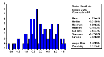
Les erreurs sont homoscédastiques

ARCH Test:
F-statistic	0.372743	Probability		0.544654
Obs*R-squared	0.386412	Probability		0.534191
Test Equation:
Dependent Variable: RESID^2
Method: Least Squares
Date: 01/27/13 Time: 14:59
Sample (adjusted): 10 196
Included observations: 46 after adjustments
Variable	Coefficient	Std. Error	t-Statistic	Prob.
C	0.798556	0.190776	4.185830	0.0001
RESID^2(-1)	0.106471	0.174393	0.610527	0.5447
R-squared	0.008400	Mean dependent var		0.862669
Adjusted R-squared	-0.014136	S.D. dependent var		1.072688
S.E. of regression	1.080243	Akaike info criterion		3.034754
Sum squared resid	51.34468	Schwarz criterion		3.114260
Log likelihood	-67.79933	F-statistic		0.372743
Durbin-Watson stat	2.276170	Prob(F-statistic)		0.544654

White Heteroskedasticity Test:
F-statistic	1.532026	Probability		0.167103
Obs*R-squared	10.42523	Probability		0.165729
Test Equation:
Dependent Variable: RESID^2
Method: Least Squares
Date: 01/27/13 Time: 15:00
Sample: 2 200
Included observations: 95
Variable	Coefficient	Std. Error	t-Statistic	Prob.
C	-27.90753	18.55292	-1.504213	0.1361
ATE	-0.046037	0.194550	-0.236633	0.8135
SEXE	0.333749	0.266417	1.252730	0.2137
LOG(AGE)	16.55577	9.769816	1.694583	0.0937
(LOG(AGE))^2	-2.217442	1.292645	-1.715430	0.0898
LOG(EMPRUN)	-0.568187	0.373366	-1.521797	0.1317
(LOG(EMPRUN))^2	0.029451	0.019539	1.507261	0.1354
ACTS	0.316683	0.203506	1.556135	0.1233
R-squared	0.109739	Mean dependent var		0.704348
Adjusted R-squared	0.038109	S.D. dependent var		0.877106
S.E. of regression	0.860230	Akaike info criterion		2.617219
Sum squared resid	64.37969	Schwarz criterion		2.832283
Log likelihood	-116.3179	F-statistic		1.532026
Durbin-Watson stat	2.358782	Prob(F-statistic)		0.167103