Relation inflation-chômage: une vérification empirique de la courbe de Phillips en RDC de 1990 à 2011

ANNEXE II.4-MODÈLE À CORRECTION D'ERREUR

Tableeau II.4.1 : output du modèle à correction d'erreur à la Hendry

Dependent Variable: DLTCHOM
Method: Least Squares
Date: 11/30/13 Time: 15:28
Sample (adjusted): 1991 2011
Included observations: 21 after adjustments
Variable	Coefficient	Std. Error	t-Statistic	Prob.
C	2.294032	0.798374	2.873380	0.0105
DLTINFL	0.034941	0.014358	2.433581	0.0263
LTCHOM(-1)	-0.607449	0.208458	-2.914011	0.0097
LTINFL(-1)	0.030208	0.012376	2.440922	0.0259
R-squared	0.488296	Mean dependent var		-0.001099
Adjusted R-squared	0.397995	S.D. dependent var		0.121653
S.E. of regression	0.094389	Akaike info criterion		-1.713136
Sum squared resid	0.151459	Schwarz criterion		-1.514180
Log likelihood	21.98793	Hannan-Quinn criter.		-1.669958
F-statistic	5.407440	Durbin-Watson stat		1.953585
Prob(F-statistic)	0.008490

ANNEXE II.5- VALIDATION DU MODÈLE

Figure II.5.1 : output du test de normalité des résidus de Jarque-Bera

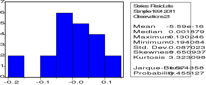
Tableau II.5.2 : output du test d'hétéroscédasticité de White

Heteroskedasticity Test: White
F-statistic	1.348344	Prob. F(9,11)		0.3151
Obs*R-squared	11.01517	Prob. Chi-Square(9)		0.2747
Scaled explained SS	8.384707	Prob. Chi-Square(9)		0.4959
sTest Equation:
Dependent Variable: RESID^2
Method: Least Squares
Date: 01/05/14 Time: 14:36
Sample: 1991 2011
Included observations: 21
Variable	Coefficient	Std. Error	t-Statistic	Prob.
C	-4.933231	4.072778	-1.211269	0.2512
DLTINFL	0.184123	0.084852	2.169928	0.0528
DLTINFL^2	-0.002509	0.001373	-1.827245	0.0949
DLTINFL*LTCHOM(-1)	-0.045266	0.021978	-2.059628	0.0639
DLTINFL*LTINFL(-1)	-0.000440	0.001482	-0.296938	0.7720
LTCHOM(-1)	2.567833	2.083548	1.232433	0.2435
LTCHOM(-1)^2	-0.336292	0.267122	-1.258943	0.2341
LTCHOM(-1)*LTINFL(-1)	0.023616	0.019846	1.189934	0.2591
LTINFL(-1)	-0.072201	0.071348	-1.011960	0.3333
LTINFL(-1)^2	-0.001880	0.001067	-1.762703	0.1057
R-squared	0.524532	Mean dependent var		0.007212
Adjusted R-squared	0.135512	S.D. dependent var		0.011264
S.E. of regression	0.010473	Akaike info criterion		-5.974227
Sum squared resid	0.001207	Schwarz criterion		-5.476836
Log likelihood	72.72939	Hannan-Quinn criter.		-5.866281
F-statistic	1.348344	Durbin-Watson stat		1.748279
Prob(F-statistic)	0.315095

Tableau II.5.3 : output du test de RESET de Ramsey

Ramsey RESET Test:
F-statistic	3.497862	Prob. F(1,16)		0.0799
Log likelihood ratio	4.152038	Prob. Chi-Square(1)		0.0416
Test Equation:
Dependent Variable: DLTCHOM
Method: Least Squares
Date: 11/30/13 Time: 15:32
Sample: 1991 2011
Included observations: 21
Variable	Coefficient	Std. Error	t-Statistic	Prob.
C	2.586407	0.761697	3.395584	0.0037
DLTINFL	0.026323	0.014177	1.856798	0.0818
LTCHOM(-1)	-0.685352	0.199055	-3.443034	0.0033
LTINFL(-1)	0.041327	0.012995	3.180130	0.0058
FITTED^2	-5.152058	2.754733	-1.870257	0.0799
R-squared	0.580094	Mean dependent var		-0.001099
Adjusted R-squared	0.475118	S.D. dependent var		0.121653
S.E. of regression	0.088136	Akaike info criterion		-1.815614
Sum squared resid	0.124287	Schwarz criterion		-1.566919
Log likelihood	24.06395	Hannan-Quinn criter.		-1.761641
F-statistic	5.525945	Durbin-Watson stat		1.801644
Prob(F-statistic)	0.005452

Tableau II.5.4 : output du test LM de Breusch-Godfrey

Breusch-Godfrey Serial Correlation LM Test:
F-statistic	1.756087	Prob. F(2,15)		0.2064
Obs*R-squared	3.984171	Prob. Chi-Square(2)		0.1364
Test Equation:
Dependent Variable: RESID
Method: Least Squares
Date: 11/30/13 Time: 15:34
Sample: 1991 2011
Included observations: 21
Presample missing value lagged residuals set to zero.
Variable	Coefficient	Std. Error	t-Statistic	Prob.
C	-3.124822	1.969509	-1.586599	0.1335
DLTINFL	0.002738	0.015616	0.175359	0.8631
LTCHOM(-1)	0.816679	0.514333	1.587840	0.1332
LTINFL(-1)	-0.030661	0.021128	-1.451234	0.1673
RESID(-1)	-0.972394	0.590712	-1.646139	0.1205
RESID(-2)	-0.501630	0.308301	-1.627076	0.1245
R-squared	0.189722	Mean dependent var		-5.76E-16
Adjusted R-squared	-0.080370	S.D. dependent var		0.087023
S.E. of regression	0.090452	Akaike info criterion		-1.733039
Sum squared resid	0.122723	Schwarz criterion		-1.434604
Log likelihood	24.19690	Hannan-Quinn criter.		-1.668271
F-statistic	0.702435	Durbin-Watson stat		1.968940
Prob(F-statistic)	0.630278

Figure II.5.2 : output du test CUSUM

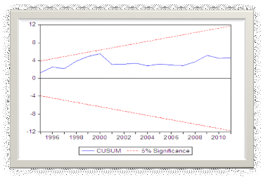
Figure II.5.3 : output du test CUSUMSQ

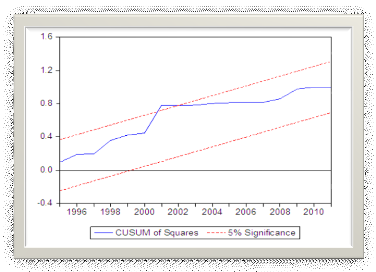
Tableau II.6 : les données utilisées pour l'estimation

Année	Taux de chômage	Taux d'inflation
1990	52,6	874,5
1991	49,4	2641,9
1992	56,3	2989,6
1993	68,7	4651,7
1994	67	9796,9
1995	69,2	370,3
1996	62,8	693
1997	53,6	13,7
1998	57,2	134,8
1999	64,2	483,7
2000	66,9	511,2
2001	49	135,1
2002	49,1	15,8
2003	48,5	4,4
2004	45,4	9,8
2005	49,4	21,3
2006	48,2	18,2
2007	47,2	9,96
2008	53,2	27,57
2009	60,8	53,4
2010	50,1	9,8
2011	51,4	23,4

Source: Banque Centrale Du Congo, Rapports Annuels (2009, 2010 et 2011) et Condencés des Informations Statistiques (2007).

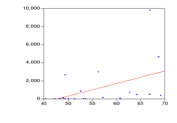
Graphique II.3- Ajustement entre l'inflation et le chômage