Contrainte Psycho-Physiques et Electrophysiologiques sur le codage de la stimulation électrique chez les sujets porteurs d'un implant cochléaire( Télécharger le fichier original )par Stéphane GALLEGO Université Lyon I - Doctorat 1999 |

par S. GALLEGO, S. GARNIER, Ch. BERGER-VACHON, CNRS - UPRESA 5020, Université Claude Bernard de Lyon L 'ESSENTIEL Ill L'implant cochléaire est un appareil qui vise à remplacer, dans l'oreille interne, la fonction de l'organe de Corti.
A la jonction de l'homme et de la machine, l'implant cochléaire recode le signal de parole. Le cerveau devra interpréter. 1. INTRODUCTION S Y N O P S I S
On connaît depuis longtemps, l'existence de liens entre l'électricité et l'audition. Dès la fin du XVIII; siècle, Volta avait remarqué qu'en mettant une différence de potentiel d'une cinquantaine de volts entre ses deux oreilles, il percevait une espèce de chuintement. Cette expérience, qui frisait l'inconscience, ouvrait, sans le savoir, un chapitre très important des relations entre la science et la santé. Par la suite, autour de l'année 1930, Stevens à Boston et Gersuri en URSS ont déclenché des sensations auditives chez des sujets sourds, en reproduisant (avec des tensions moindres) l'expérience de Volta. Une date importante est à retenir avec la travail de Clarke à Melbourne (1979) qui érigeait un principe longtemps considéré comme un dogme : "l'implant cochléaire doit transmettre les éléments qui caractérisent la phonation". Ces éléments sont classiquement le fondamental laryngé et les formants [2]. Cela a conduit à l'implant cochléaire Nucleus qui est toujours le plus diffusé sur la planète, notamment grâce à la structure commerciale et l'assistance technique mise en place sur tous les continents par la société Cochlear, filiale de la puissante compagnie Dunlop Pacific. Cette petite merveille technologique, parfaitement adaptée aux possibilités de l'électronique de 1980, a ensuite été remise en cause pour revenir au codage classique du spectre de la voix en bandes de fréquences distribuées dans l'oreille. Ce principe a été beaucoup défendu, notamment par l'école française du professeur Chouard et du physiologiste Mc Leod. L'article de référence dans la discipline, date de 1957. Il est l'oeuvre des Français Djourno et Eyries dans la Presse Médicale [1]. Les auteurs avaient produit une sensation auditive chez un sujet sourd en lui implantant une bobine délivrant sur la cochlée une tension électrique alternative. Il était donc possible de passer, en transcutané, une information depuis le milieu extérieur vers l'organe sensoriel de l'ouïe. Néanmoins, les résultats qu'ils avaient obtenus étaient d'une qualité tellement mauvaise qu'ils ne dépassaient pas le domaine de l'anecdote. Reprise aux Etats-Unis, la technique allait connaître un nouvel essor, notamment avec les travaux de House à Los Angeles qui réalisait le premier implant cochléaire portable et obtenait l'agrément de la FDA (Food and Drug Administration). Ensuite le premier congrès était organisé sur ce thème en 1973 à San Francisco. Il réunissait les chirurgiens et scientifiques interpelés par la question. Peu de temps après (1974), le professeur Chouard à l'hôpital St Antoine de Paris réalisait la première implantation en France et il prenait place parmi les pionniers de la discipline.
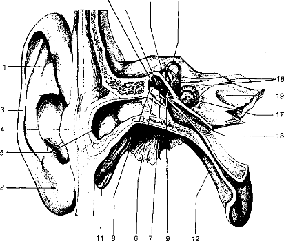
rampe vestibulaire rampe tympanique fenêtre étrier BASE APEX fenêtre I. Membrane basilaire déroulée : sélection d'une fréquence sonore.
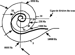
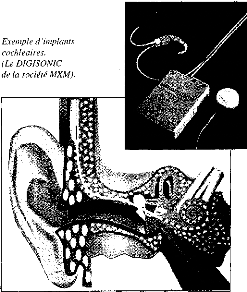
Exemple d'implants cochléaires. (Le DIGISONIC de la société MXM). L'oreille interne a pour propriété d'analyser l'onde acoustique et de la distribuer le long de la cochlée, en fonction de la fréquence qui est détectée par la membrane basilaire (figure 1).
L'implantation cochléaire s'est disséminée à grande vitesse au cours des années quatre-vingt et maintenant plus de 20 000 personnes portent cette technologie de par le monde. Quelques implants cochléaires dominent actuellement le marché mondial. Nous pouvons citer :
3. RELATION AVEC LE PATIENT Les personnes concernées par l'implant cochléaire sont porteuses de surdités profondes liées à une défaillance complète de l'organe de Corti. Dans l'oreille interne, l'organe de Corti transforme les vibrations acoustiques en un stimulus électrochimique qui est distribué sur les terminaisons du nerf auditif. Les voies de l'audition transmettent ensuite cette information vers le cortex cérébral qui va interpréter ce message comme venant du sens de l'ouïe. Cette interprétation fait appel, bien sûr, à toutes les fonctions supérieures de l'homme, à ses possibilités et à tout le passé qu'il a emmagasiné depuis sa naissance et même peut-être avant. Donc, lorsque l'organe de Corti est totalement détruit, les amplifications du signal resteront sans effet. Par contre, on peut court-circuiter sa fonction à l'aide du mécanisme décrit ci-dessus. Il est bien clair que ceci est seulement sensé copier le fonctionnement physiologique de l'oreille. selon l'état actuel de nos connaissances. Le message qui est transmis au cortex cérébral est très appauvri par rapport à celui qui arrive avec une audition normale. Il est important que le patient puisse s'y adapter. On admet donc que les conditions suivantes doivent être requises avant une implantation cochléaire :
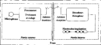
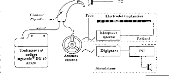
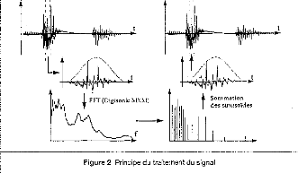
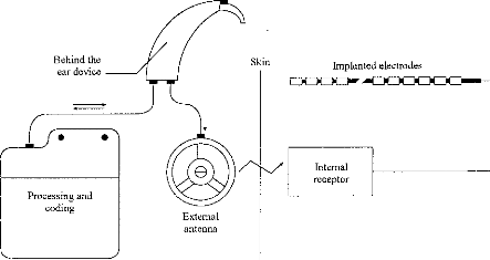
Le signal est ensuite reçu et démodulé par la partie interne. Les différentes fréquences sont détectées et l'énergie correspondante est distribuée sur les électrode réparties le long de la Cochlée, pour simuler le phénomène physiologique observé sur une cochlée normale. Considérons maintenant la partie externe. Son fonctionnement est représenté sur la figure 3. Le signal acoustique est capté par un microphone, puis amplifié. Il est ensuite décomposé selon l'énergie contenue dans les bandes spectrales réparties sur la gamme utile de l'audition. Puis cette énergie est compressée pour que la dynamique acoustique soit adaptée à la dynamique électrique des terminaisons du nerf auditif arrivant sur la cochlée. Pour chacun des canaux, une impulsion est construite. Sa surface est proportionnelle à l'énergie électrique issue de la compression logarithmique. Un séquenceur permet de construire un jeu d'impulsions séquentielles représentant l'énergie détectée dans les n canaux. Une porteuse est ensuite modulée en amplitude avec ces impulsions. De l'autre côté de la peau, les impulsions sont détectées de manière séquentielle et distribuées le long de la cochlée les unes après les autres. Cette stratégie est désignée sous le nom de CIS (Continuous Interleaved Samples). Actuellement, le fonctionnement décrit figure 3 est réalisé numériquement [5]. Le signal d'entrée est échantillonné, puis une FFT permet de déterminer, à l'aide de raies, sa structure spectrale. Les raies sont ensuite rassemblées en bandes avant d'attaquer la compression logarithmique. Ce mode de fonctionnement est très répandu ; il correspond notamment à celui qui est effectué par l'implant français Digisonic [5]. 52 I REE N° 8 5z Septembre 1997 mieux comprendre et faire évoluer une technique coûteuse et qui fait appel aux fonctions supérieures de l'homme. Autant pour la Société que pour le Patient, on doit tirer le meilleur parti des systèmes de traitement du signal très ouverts qui sont actuellement mis en place. Remerciements Les auteurs remercient les organismes et personnes qui soutiennent leur recherche, la société MXM, le groupement GIPA, les Hospices Civils de Lyon et le CNRS, ainsi que les professeurs L. COLLET, A. MORGON et E. TRUY de l'Hôpital Edouard Herriot de Lyon. Bibliographie
Stéphane GALLEGO prépare une thèse de doctorat en génie Biomédical sur les mesures objectives avec l'implant cochléaire au laboratoire "Neurosciences et systèmes sensoriels". CNRS UPRESA 5020 de l'Université Claude Bernard de Lyon. Stéphane GARNIER prépare une thèse de doctorat en génie Biomédical sur l'évaluation de la perception du signal acoustique au laboratoire "Neurosciences et systèmes sensoriels". CNRS UPRESA 5020 de l'Université Claude Bernard de Lyon. Christian BERGER-VACHON est professeur d'Instrumentation Médicale au laboratoire "Neurosciences es systèmes sensoriels". CNRS UPRESA 5020 de l'Université Claude Bemard de Lyon.
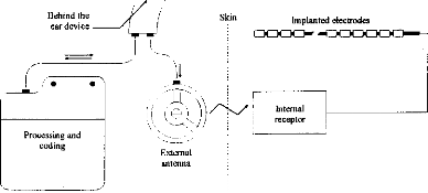
On ne peut pas se contenter de poser cette technologie sans essayer de la faire évoluer. De plus, le suivi des résultats du patient et l'adaptation de la stratégie de codage sont des éléments importants conditionnant la réussite ou l'échec de l'implantation. Le spécialiste du traitement du signal a donc totalement sa place dans le groupe de prise en charge des personnes implantées, avant et après le geste chirurgical, voire même pendant si on veut vérifier en temps réel au bloc opératoire le bon fonctionnement de l'appareil lors de sa mise en place. 4. CONCLUSION La lutte contre le handicap associé à une surdité profonde ou totale, en employant la thérapeutique de l'implant cochléaire, fait appel à une prise en charge du patient très rigoureuse. Il y a d'une part l'aspect médical (médecin, chirurgien) et paramédical (orthophoniste, audioprothésiste, psychologue, technicien) et d'autre part l'aspect scientifique pour II/L'implant cochléaire Digisonic®a/ Description Le Digisonic® DX10 est un implant cochléaire multicanal destiné à la réhabilitation des surdités cochléaires bilatérales profondes ou totales. Cet implant, de type transcutané, comprend : un émetteur (ou processeur) externe relié à un capteur de son (microphone) et à une antenne externe qui transmet, par couplage électromagnétique, le signal acoustique traité par le processeur, à un récepteur- stimulateur implanté sous la peau derrière le pavillon de l'oreille. Le récepteur-stimulateur est connecté à un porte-électrodes inséré dans la cochlée (oreille interne). Le Digisonic ® DX10 comprend 15 électrodes actives. Chaque électrode stimule différents contingents de fibres nerveuses auditives et est associée à une bande de fréquence du signal sonore traité par le processeur externe. Le boîtier récepteur-stimulateur et l'antenne externe contiennent un aimant. L'antenne externe est ainsi maintenue en regard de l'implant par attraction magnétique. Le récepteur-stimulateur ne contient pas d'alimentation électrique propre, il reçoit l'énergie nécessaire à son fonctionnement par couplage électromagnétique. Ainsi lorsque l'antenne externe n'est pas positionnée en regard du récepteur implanté, l'implant est passif.
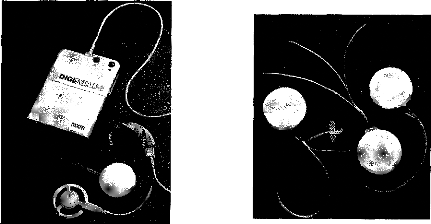
Le processeur Digisonic ® est entièrement numérique. Cette technologie permet une re-programmation complète du processeur. L'audiologiste peut ainsi mettre à jour les versions logicielles de traitement du signal permettant au patient de bénéficier des nouvelles stratégies de codage sans changer de processeur. Actuellement trois produits sont disponibles (figure 10). - Un implant cochléaire composé d'un porte-électrodes comprenant 15 électrode actives, utilisé pour les implantations cochléaires classiques. - Un implant cochléaire composé de 3 porte-électrodes. Il est utilisé principalement lorsque la cochlée du sujet est ossifiée. La répartition des électrodes (4,4,4 ; 6,5,4 ...) varie selon le patient à implanter. On passe un porte-électrode par voie normale (proche ou via la fenêtre ronde), les deux autres porte- électrodes sont insérés par cochléostomie. - Un implant du tronc cérébral dont le porte-électrode est composé d'une grille de 15 électrodes que l'on vient poser sur le noyau cochléaire. Il est utilisé lorsque le patient a subi une neurotomie vestibulaire bilatérale sans restes auditifs. Le nerf auditif étant sectionné, un implant cochléaire serait inefficace. L'implant du tronc cérébral pourrait aussi être envisagé lorsque la cochlée est très ossifiée. Le traitement du signal par implant cochléaire a pour objet de transmettre l'information acoustique aux ganglions spiraux. Il s'agit d'extraire de la parole les éléments les plus informatifs, de les coder et de les rendre accessibles aux voies nerveuses via les électrodes. La quantité d'information transmise par l'implant et intégrée par le sujet est très inférieure à celle disponible lors du fonctionnement normal de la cochlée. Le premier objectif du traitement de signal est de sélectionner en amont les éléments les plus informatifs de la parole. L'énergie du signal de parole se situe principalement dans les basses fréquences (inférieur à 1 kHz) alors qu'une bonne partie de l'intelligibilité est contenue dans le domaine des fréquences de 1 à 4 kHz (Gelis, 1993, Calliope, 1989). Il est donc important d'équilibrer en énergie les différentes bandes fréquentielles pour éviter des phénomènes de masquage. b/ Traitement de signal Le DIGISONIC® effectue une Transformée de Fourier Rapide (FFT : Fast Fourier Transform). La fenêtre d'analyse est de 8 ms, et on utilise un recouvrement par fenêtre de Hamming de 50 % afin de ne pas détériorer l'enveloppe du signal (Caliope, 1989). La transformation FFT de l'implant Digisonic ® calcule 64 filtres en temps réel d'une largeur de 122 Hz, entre 122 et 7800 Hz. Ces filtres sont regroupés en au plus quinze plages de fréquences centrées sur les valeurs moyennes des bandes critiques de la cochlée (Caliope, 1989). Ces plages fréquentielles sont affectées aux 15 électrodes actives de l'implant (figure 11). Energie (dB) 15 bandes de fréquence ajustables 64 valeurs d'énergie (FFT) 100 -+F-- 122 Hz 7800 Freq (Hz) Figure 11: La Transformée
de Fourier du Digisonic® et la distribution cl Codage de la stimulation Les stimulations doivent apporter à chaque population de neurones une énergie compatible avec leur densité et leur localisation tonotopique. Cette énergie se situe entre un minimum et un maximum correspondant à une sensation liminaire et une sensation de confort. Les variations d'énergie acoustique de chaque plage fréquentielle vont piloter l'énergie électrique des électrodes correspondantes. L'activation d'une électrode dépendra de la détection d'un pic d'énergie dans la plage fréquentielle qui lui est allouée. L'intensité de la stimulation électrique dépend de la quantité de charges électriques injectées dans le milieu. Cette quantité de charges est elle-même le produit de l'amplitude de l'impulsion de stimulation électrique et de la largeur de l'impulsion (ou durée). Sur le Digisonic, la durée de l'impulsion a été choisie comme paramètre permettant de faire varier la quantité de charges électriques (1 à 620 ps). Cette méthode a l'avantage de stimuler toujours la même zone tonotopique de la cochlée, ce qui n'est pas le cas lorsqu'on choisie de faire varier l'amplitude. En revanche, l'amplitude peut être modifiée en fonction des spécificités de chaque sujet (de 0.5 à 3 mA).
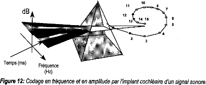
Fréquence Figure 12: Codage en fréquence et en amplitude par l'implant cochléaire d'un signal sonore. La quantité de charges injectée sur les électrodes est déterminée par la composition fréquentielle du signal sonore capté (figure 13), puis adaptée de façon à être comprise entre le seuil de perception du patient (ou seuil minimum) et son seuil de confort (ou seuil maximum) déterminés lors du réglage pour chacune des électrodes actives (15 au maximum). Microphone externe
Dynamique acoustique d'entrée: 40-90 dB Dynamique électrique cochléaire: 2-12 dB Figure 13: Principe de la compression de la dynamique (acoustique/électrique) Max Min Pour chaque électrode (canal) la dynamique acoustique d'entrée doit être comprimée et ajustée à la dynamique étroite de stimulation électrique cochléaire. La fonction de compression permettant le transfert de l'énergie acoustique en énergie électrique est logarithmique, ce qui reproduit bien la fonction de transfert de la cochlée (compression logarithmique au niveau de la membrane basilaire ; Leipp, 1977). Afin d'adapter la compression au sujet, la puissance du logarithme est variable. Une seule électrode est active à la fois: c'est le principe de la stimulation séquentielle (non-simultanée) qui permet de minimiser les interactions inter-électrodes (figure 14). La période ou rythme de stimulation (Tstim), c'est-à-dire l'intervalle de temps séparant deux impulsions sur la même électrode, est soit proportionnelle au fondamental laryngé (F0) lorsque celui-ci est détecté, soit fixée à une valeur programmable lorsqu'il n'est pas détecté. Durant cette période la stimulation successive de stimulation des différentes électrodes est appelé trame. SPECTRE 7800 Hz ELECTRODES _ib. 15 100 Hz -41 Tstim Temps Figure 14 : Principe du codage séquentiel de la stimulation d/ Sensibilité acoustique Pour s'adapter à la structure acoustique de l'information de parole, Le Digisonic® traite un spectre énergétique compris en moyenne entre 45 et 85 dB, et un spectre fréquentiel compris entre 122 et 7800 Hz. Le seuil de détection peut être choisi selon le sujet porteur de l'implant entre 32 et 68 dB. Afin d'éviter un masquage de l'information dans les milieux bruyants le Digisonic® permet, par l'utilisation d'un réglage de sensibilité acoustique progressive et différenciée, de favoriser la plage aiguë en diminuant l'énergie de la zone grave et en augmentant le seuil de déclenchement. C'est le patient qui le gère au moyen de bouton poussoir + et -.
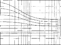
dB 65 60 55 50 45 40 35 Pos 1 2 3 4 5 9 100 1000 10000 Hz Figure 15 : Sensibilité progressive et différenciée (BF/HF): Réseau de courbes (9 positions) e/ Répartition fréquentielle La flexibilité du système permet d'adapter la répartition fréquentielle à chaque sujet implanté. Cela est très utile, en particulier pour l'implant cochléaire multi porte-électrodes et l'implant du tronc cérébral, pour lesquels il est nécessaire de rechercher une tonotopie qui ne suit plus le numéro des électrodes.
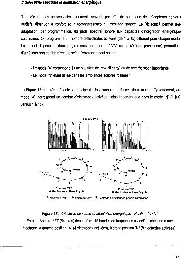
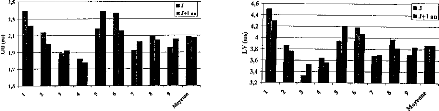
Figure 16 : Exemple de répartitions fréquentielles sur un implant cochléaire (gauche) et un implant du tronc cérébral (droite). Chaque électrode active, représentée en ordonnée, code un spectre acoustique bien défini, représenté en abscisse Il existe sur chaque canal la possibilité d'ajuster le gain acoustique afin d'affiner l'équilibre énergétique de tous les canaux.
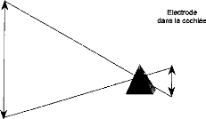
5 3 11 4 --)(-- 122 Hz 3 Position "N" 8 électrodes actives / cycle Position "A" 4 électrodes actives / cycle 122 Hz 7900 Fre9 (Hz) 100 Hz 14 8 kHz 2 1 Y Y hi 11 15 Y Y Y 12 13 15 4 ° électrode "off' Figure 17 :
Sélectivité spectrale et adaptation
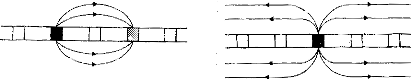
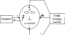
énergétique - Position "A / N" 32 g/ Tonalité Il est possible de modifier globalement la sensation de tonalité pour ajuster la perception de hauteur des voix de manière à les rendre plus naturelles pour le patient. On propose 10 positions dans ce menu de réglage. Cela correspond à une variation fine de la fréquence moyenne de stimulation comprise entre 125 et 410 Hz. Le patient doit indiquer ce qui lui paraît le mieux adapté à sa perception normale en faisant référence à sa mémoire auditive, quand cela est possible. h/ La stimulation électrique de l'implant cochléaire Digisonic La stimulation électrique de l'implant cochléaire peut se faire de différentes façons (figure 18). L'implant cochléaire Digisonic® utilise une stimulation de type masse-commune (une électrode positive, toutes les autres sont à la masse). Une autre électrode extracochléaire permet de décharger les capacités après stimulation, mais n'a que peu d'effet sur la stimulation cochléaire. Dans l'étude qui va suivre nous l'avons négligée pour faciliter les calculs.
in
Active Return E] Inactive electrode current electrode Figure 18 : Différents
modes de stimulation. Bipolaire : stimulation entre deux électrodes
intra- Article 2 :MODELLING OF THE ELECTRICAL STIMULATION DELIVERED BY
THE
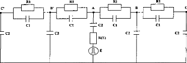
| |||||||||||||||||||||||||||||||||||||||||||||||||||||||||||||||||||||||||||||||||||||||||||||||||||||||||||||||||||||||||||||||||||||||||||||||||||||||||||||||||||||||||||||||||||||||||||||||||||||||||||||||||||||||||||||||||||||||||||||||||||||||||||||||||||||||||||||||||||||||||||||||||||||||||||||||||||||||||||||||||||||||||||||||||||||||||||||||||||||||||||||||||||||||||||||||||||||||||||||||||||||||||||||||||||||||||||||||||||||||||||||||||||||||||||||||||||||||||||||||||||||||||||||||||||||||||||||||||||||||||||||||||||||||||||||||||||||||||||||||||||||||||||||||||||||||||||||||||||||||||||||||||||||||||||||||||||||||||||||||||||||||||||||||||||||||||||||||||||||||||||||||||||||||||||||||||||||||||||||||||||||||||||||||||||||||||||||||||||||||||||||||||||||||||||||||||||||||||||||||||||||||||||||||||||||||||||||||||||||||||||||||||||||||||||||||||||||||||||||||||||||||||||||||||||||||||||||||||||||||||||||||||||||||||||||||||||||||||||||||||||||||||||||||||||||||||||||||||||||||
|
E o 2000 U C 1500 E 1000 "FI C |
3.0 3.5 4.0 4.5 5.0 5.5 6 0
Power supply voltage (Volt)
Figure 3 : Impedance of the output transistor with respect to the output voltage when the load is 1 kohm (full dots) and 10 kohms (empty squares).
The next step was to compare the two models when the pulse duration varied. The experimental range was from 5 to 320 gs and the steps were exponentially increased. Figure 4 indicates the voltage VI given by the first model. Figures Sa and 5b show the simulation of VI and V2 by the second model. VI (V(1,3) and V(1,5)) are very similar for the two models. V2 is mostly lower than VI when the duration of the excitation pulse is below 80 gs.
|
1.0 0.8 0.6 0.4 0.2 0.0 -0.2 -0.4 -0.6 |
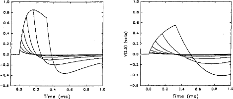
Figure 4: V(1, 3) obtained from the 3-pole model, with the pulse duration (t=5, 10, 20, 40, 80, 160, 320 ,us) taken as a parameter. The load had the physiological value of 2 kohms and Cl was 100 nF (E=3.35 volts, R(E)= lkohm). The curve on the right refers to 320 ,us. |

0.0 0.2 0.4 0.6 0.8 10
Time (ms)
1.0
0.8
0.6
0.4 0.2 0.0 -0.2 -0.4 -0.6
0.0 0.2 0.4 0.6
Time (ms)
-0.2
-0.4
-0.6
0.8 1 0 0.0 0.2 0.4 0.6
Time (ms)
0.8
0.6
1.0
0.2
10
0.8
Fig V(1, 5), VA-VB, simulation (5 pole
mode!) with respect to the pulse duration (1=5, 10, 20, 40, 80, 160, 320 us). The load had a physiological value of 2 kohms and Cl was 100 nF (E=3.35 volts, R(E)= lkohm).
Figure 5b: V(2,5), VB-VC, simulation (5- pole model) with respect to the pulse duration (1=5, 10, 20, 40, 80, 160, 320 ,us). The load had a physiological value of 2 kohms and Cl was 100 tiF (E=3.35 volts, R(E)= lkohm)
In normal conditions, the impedance of the physiological medium does not vary significantly. But, in special circumstances, for instance in the case of partially ossified cochlea, impedance is increased on some electrodes. Figures 6a and 6b show the evolution of the impulsion voltage (using the second model) respectively considering the resistance R1 and the capacity C l. The
duration of the excitation pulse was kept below 80 lis. Variation of the response (shape and amplitude) was high with respect to C I (figure 7). On the contrary, the influence of RI was rather small. The time to reach the maximum of the output pulse followed the value of R1.
0.8
10
0.0 0.2 0.4 0.6
Time (ms)
-0.2 '
0.0
0.2
0.4
Time
0.6
(ms)
0.8
10
1.0
0.8
0.6
0.4
0.2
0.0
1.5
1.2
0.9
0.6
0.3
0.0
-0.3
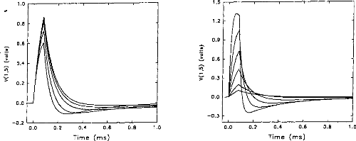
Figure 6a: V(1,5) simulation (5-pole model), Figure 6h: V(I,5) simulation (5-pole mode!),
with respect to the load resistance (RI = 1, 2, when the condenser had the following values.
5,
· 10, 20 kohms) where Cl = 100nF. (E=3.35 (CI =20,
50, 100, 200, 500, 1000 nj9 where
volts, R(E)= I kohm). The higher the RI=2kohms. (E=3.35 volts, R(E) = I kohrn).
impedance, the greater the amplitude. The smaller the CI, the higher the amplitude.
It is possible to calculate the electrical charge delivered to the medium taking the integration of the positive part of the pulse and a division by Rl.
fp
21V i(t)dt
U- ° R1 where V1(t0)=0.
The amount of electricity denoted Q, has been calculated in different situations, where the excitation pulse duration and the medium impedance varied. Results are given in figures 7 (first model) and 8 (second model). Results show that Q was linearly increased until an excitation duration of 160 jis caused saturation. The same trend was observed with respect to the
medium resistance. Both models led to equivalent results for pulses shorter than 320 las and with a capacity C2 less than 500 nF (Q2/Q1<ldB) (figure 9).
C 20 nr
· C 50 ni'
ü C- 100 sir
· C 800 nr
q C 600 nr
n C 1000 ni'
1 000
· 100 10
(t)
1
_c
U
10
100
1000
· R = 1000 ohms
· R - 2000 ohms
· R na 6000 ohm. a R - 10000 ohm.
n R 20000 ohms
0.1
1000
· 100
o
o
10
L.
o 1 _c
0.1
10 100 1000
Pulse duration (j s)
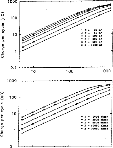
Figure 7: Load delivered hy the electrodes B and B' calculated using the 3-pole model, with respect 10 the pulse duration when several values qf CI (top, R1=2 kohms), or RI (bottom, Cl - 100 nF) are used (E=3.35 volts, R(E) =1 kohm):
1
0.1
10
100
1 000
1000
100
20 nr
C 50 nr
C 100 nr
C 800 nr
C-- 500 nr
C 1000 nr
1 0
· R = 1000 ohm.
· R int 2000 ohm,
· R ms 5000 ohm.
o R 10000 ohms
n R 20000 ohms
0) Cn
o 1
-C
0.1
1000
10 100 1000
Pulse duration (m,$)
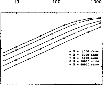
Figure .8: Load delivered hy the electrodes B and B' calculated using the 5-pole model, with respect to the pulse duration when several values of Cl (top, R1=2 kohms), or RI (bottom, C1=100 nF) are used (E=3.35 volts, R(E) = 1 kohm).
49
. 0
c
· y
0.5
0.0
Ol
o
O
C`4 --0.5
1.5
--1.0
10
100
1000
R = 1000
· 2000
R = 5000
· = 10000
· 20000
10 100
Pulse duration (gs)
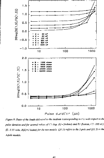
Figure 9: Ratio of the loach delivered 10 the medium (corresponding to VI) with respect to the pulse duration and for several values of CI (top, RI =2kohms) and RI (bottom, (' I 100 id), (E=3.35 volts, R(E) = I kohm) for the two models. Q(1, S) refers to the 5-pole and 0(1,3)10 the 3-pole models.
|
2.0 |
|
|
ri, |
1.5 |
|
1.11 |
1.0 |
|
rn |
|
|
0 |
0.5 |
|
0.0 |
Discussion
Comparison of the two models
The comparison of the results given by the two models showed a high similitude for the shape and values of the charges delivered by the DIGISONIC DX10 cochlear implant when the excitation pulse was shorter than 320 gs. When the decimal logarithm was equal to 1, the ratio of charges was 1.12, which is practically equivalent to 1. This could mean that the excitation path is very short and does not spread throughout the electrodes. Consequently, a 3-pole circuit appears adequate to provide a good model of the stimulation. At least, a 5-pole model did not lead to different results. A special non-symmetrical model needs to be established for the side electrodes (1 and 15).
Influence of the physiological medium impedance
The shape of the response was significantly influenced by the impedance of the physiological medium between two electrodes. In this case, it seemed that information about the status of the active electrode couid only be obtained by considering the surface potentials in cochlear implantees (Mens et al, 1994; Gallégo et al, 1997). Surface potentials were potential differences recorded between surface electrodes situated on the skin. They were produced by the electrical action of the implant electrodes. They couid be interpreted by the action of a stimulation dipole situated on the line connecting the recording electrodes.
One application could be to help set the liminar and comfort thresholds on each electrode. The more ossified the cochlea, the higher the impedance. Consequently, in the case of ossification, an increase of the liminar thresholds and a reduction of the electrical dynamic couid be seen. If we consider figure 6a, it can be seen that the offset time, from the peak to the baseline, is a function of the impedance, which consequently could be evaluated.
Choice of the skin electrodes
If the line connecting the two skin electrodes, E 1 and E2 is orthogonal to the dipole, the action of the dipole is the same on El and E2. Consequently the potential difference is null. In all other cases, this potential difference is not equal to zero (fig 10).
|
El |
E2 |
Dipole
Figure 10 : Schematic representation of the skin electrodes relative to an exciting dipole.
Influence of pulse duration
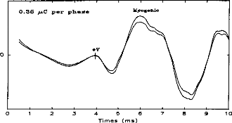
Figure 11 shows a typical surface potential. Waveform is modified by the bandpass of an analog filter on the recording system (10-3000 Hz).
100 80 60 40 20 0
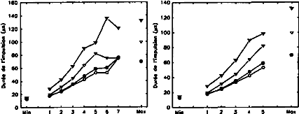
ce --20
--40 -
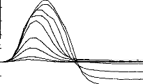
Figure 11: Surface potentials VE1-VE2 recorded on a cochlear implant subject with regard to pulse duration (1=5, 9, 22, 34, 60, 86, 137, 188, 239 ps).
|
0 0 0.1 0.2 0.3 0.4 0.5 0.6 Time (ms) |
0.7 0.8 0.9 1 0 |
The amount of charge delivered by the implant grew linearly with the duration of the pulse. It has been shown (Shannon, 1992) that an increase in perceived volume is proportional to the electrical charge delivered to the medium between two electrodes. It has also been established, with normal hearing people, that the perceived volume is in proportion to the acoustic stimulation given in decibels. In other words, the stimulation growth should be proportional to the duration of the pulse. Following these considerations a logarithmic compression of the acoustical pressure could be converted to a pulse duration. The introduction of condensers did
not increase the difficulty of evaluating the charge delivered by the electrodes. The maximum
charge delivered by an electrode is, according to figures 7 &8, less than 1 giC. The surface of the electrode is about one square millimetre, and the charge density in the tissue is less than 1 itC/mm2. These charges remain well below the safety limit established in order to assure the integrity of the physiological tissues (40iic per square millimetre and per cycle).
Further developments of the model
Considering the remote action (on the skin) of electrical stimulation seen so far, this model may be considered as a first step toward a more complete one. The next step in this modelling would be to extend the models to 'in vitro' and 'in vivo' situations (figure 10), with corresponding measurements. This would help the localisation of the stimulation on the cochlea, the assessment of the quality of the implanted device and the measurement of the electrode impedances.
In our model, the system was even more complicated by the fact that two dipoles must be considered when the stimulation is symmetrical (in the 3-pole or the 5-pole representation). This situation will be considered in a further step of the modelling.
Conclusion
The present study shows that a 3-pole model provides an adequate means of representing the electrical stimulation delivered by a cochlear implant used in a common ground mode. The extension to a 5-pole model did not really change the results.
The influence of the medium resistance modified the shape of the stimulation. Consequently, the knowledge of the impulse response indicates the status of the medium, mostly in the case of ossification. The recording of the electrical response produced by a pulse indicates also the amount of electricity delivered between two electrodes. The relation is non linear and the shape has to be seen to evaluate the magnitude of the stimulation.
The next step would be to use this 3-pole model in order to
simulate the surface potentials on
the skin. The relation between the
prediction and the observed values will determine the power
of the model, model which is of the utmost importance to establish the cochlear implant working mode and the status of the physiological medium surrounding the electrodes.
Acknowledgments
The authors acknowledge the people and institutions supporting their work: the MXM society, the Hospices Civils of Lyon, the CNRS, the University of Lyon and Professor Lionel Collet Director of the laboratory.
References
- Beliaeff M., Dubus P., Leveau J.M., Repetto J.C., Vincent P. Sound Processing and Stimulation coding of DIGISONIC DX10 15-channel Cochlear Implant. Advances in cochlear implant, Ed. IN Hochmair (Innsbruck). 1994;198-203.
- Black R, Clark G, Tong Y, Patrick J. Current distributions in cochlear stimulation. Ann NY Acad Sci, 1983, 405, 137-145.
- Fravel R. Cochlear implant electronics made simple. Otolaryngol Clin North Am, 1986, 19, 11-22.
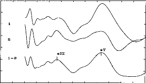
- Gallégo S, Truy E, Morgon A, Collet L. EABRs and surface potentials with a transcutaneous
multielectrode cochlear implant. Acta Otolaryngol (Stockh), 1997, 117 (in press).
· - Mens LHM, Oostendorp T, Broek P van den.
Identification Electrode Failures with Cochlear
Generated Surface Potentials. Ear Hear 1994;15, 330-338.
- O'Leary S, Black R, Clark G. Current distributions in cat cochlea: a modelling and electrophysiological study. Hear Res, 1985, 18, 273-281.
- Shannon R. Multichannel electrical stimulation of the auditory nerve in man. I. Basic psychophysics. Hear Res, 1983, 11, 157-189.
- Townshend B, Cotter N, Van Compernolle D, White R. Pitch perception by cochlear implant subjects. J Acoust Soc Am, 1987, 82, 106-115.
53
Le réglage de l'implant a pour but de sélectionner les électrodes fonctionnelles et de déterminer pour chacune d'entre elles les seuils d'énergie électrique qui produiront une sensation liminaire et une sensation confortable.
Une étude (E. Truy, S. Gallégo, C. Berger-Vachon & L. Collet, 1995) a montré que la désactivation des électrodes qui n'apportent pas d'information supplémentaire améliore la performance des sujets, même dans les cas les plus défavorables ou le nombre d'électrodes actives est déjà réduit (cochlées ossifiées). Le point clé de l'adaptation d'un implant est donc de ne conserver que les électrodes susceptibles d'apporter une information différenciée et harmonieuse. Chaque électrode doit correspondre à une sensation de hauteur tonale différenciée et transmettre un nombre de pas en sonie suffisant et équilibré entre les différents canaux.
Le nombre d'électrodes différenciées détermine les plages fréquentielles, et les pas de sonie définissent les limites de la plage énergétique acoustique correspondante.
b/ Chronologie du réglage
Deux paramètres du réglage doivent être distingués. Le premier comprend tout ce qui a trait à la stimulation électrique : seuil de détection, seuil de confort, nombre de canaux, nombre de canaux ouverts par trame ... Le second comprend tout ce qui se rapporte à l'information acoustique : répartition fréquentielle, gain, compression, seuil de déclenchement...
1/ Réglage des paramètres électriques
Mesure des seuils
La première étape d'un réglage consiste à ajuster les paramètres de l'interface bio-électrique entre le patient et l'implant cochléaire pour chaque électrode.
Cela se traduit dans un premier temps par :
- La détermination des seuils de perception (Min)
- La détermination des seuils de confort (Max)
|
REGLAGE DE5 SEUILS Man du patient BEETHUOEM |
||||||||||||
|
1 |
ner . e.,:-: |
. -2 00 881 00 801 00 001 00 001 08 801 00 801 00 081 00 081 00 801 80 001 00 001 08 001 08 081 ee 081 |
.ln 824 826 825 824 028 818 BOO 088 800 888 MO |
037 043 048 049 044 035 025 808 01:10 cee |
do 06 04 86 86 86 05 e5 05 03 In In In ln |
|||||||
|
eM00 |
||||||||||||
|
010 858 080 0% a . 2 sh Biton: Stim alternée - Ctr1.11: Blette référence - Ffe. Remi d la uoix Fi: I. - F3: Bal - F5: Ulm f - F9: Sauu - F18 : Fin |
||||||||||||
|
1MW-Cifrai,114(1-lalt1 1171`4 |
||||||||||||
|
REGLRGE MU SEUIL, Mon du pdt Lund LEETHOL Il |
||||||||||||
|
IS |
019837 |
|||||||||||
|
BO I, 9- .sur les électrode=1 |
||||||||||||
|
039 |
||||||||||||
|
Min 10 gp 5ex 70. 02 Max 128% QI MM MM MM MM MM MI Taper sur une tourne pour arrêter la etimulaticm |
043 848 els 035 |
|||||||||||
|
080 |
1 |
|||||||||||
|
ee eet 09 eet 88 001 |
BOO ace 880 |
888 (ne |
1 1 I I |
|||||||||
|
FI. |
Sh Alt.12. e 038 048 869 0 800 180 Type etim - F7 . Réglage gaine - Fe. Modification globale dee eeull Stim alternée - Ctrl I. - F3: Bal - IS: Uieu f - F9: Sein - F18 : Fin 1
|
|||||||||||
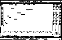
Figure 19 : Ecran de réglage des seuils Min et Figure 20: Balayage des canaux à différents
Max pour une amplitude donnée niveaux
Equilibre en sonie de chaque canal
Une fois les seuils déterminés, on réalise un équilibre de la fonction de sonie entre les différents canaux. On utilise pour cela un balayage de toutes les électrodes ou une stimulation alternée entre deux électrodes différentes à un pourcentage de la dynamique donné (0, 10, 30, 50, 70, 90, 100, 120 %). Le patient indique les variations de sonie évoquées par le balayage des électrodes.
La chronologie est la suivante:
- On équilibre les Maxima (100%) en diminuant le niveau des électrodes les plus fortes et en augmentant le niveau des électrodes les plus faibles pour qu'elles soient toutes perçues au même niveau de sonie,
- On équilibre les Minima (0%) en augmentant le niveau des électrodes qui ne sont pas perçues pour qu'elles soient toutes au même niveau,
- On équilibrage les seuils à 30% et 70 % de la dynamique en jouant sur les Minima et les Maxima.
S'il apparaît qu'une électrode ne peut pas être équilibrée correctement avec les autres on peut envisager sa suppression ou une augmentation globale de l'amplitude des impulsions si la dynamique est importante.
Différentiation tonotopique des électrodes
Il est indispensable de mesurer la hauteur tonale de chaque canal. Pour cela chaque électrode est comparée à la précédente à 50 % de sa dynamique. Le patient indique quelle est la plus aiguë. Une électrode perçue identique à la référence sera inactivée car elle n'apporte pas d'information différentiée.
En pratique, tant que le nombre d'électrodes actives n'est pas inférieur à 8, le codage du spectre de la parole reste satisfaisant.
Ces différentes étapes nous permettent d'obtenir toutes les informations nécessaires à l'interface bioélectrique.
2/ Réglage des paramètres acoustiques
Le principe de la seconde étape est d'ajuster les paramètres permettant l'adaptation du signal acoustique au signal électrique.
Répartition fréquentielle
Le paramètre le plus important à régler est le domaine spectral attribué à chaque électrode (figure 16). Des valeurs sont données par défaut avec répartition des fréquences selon l'échelle Bark (linéaire puis logarithmique). Il est parfois utile, surtout avec l'implant multi porte-électrode et l'implant du tronc cérébral, de pouvoir les modifier et les adapter aux spécificités du patient. Il s'agit de trouver un compromis entre l'intelligibilité que peut apporter une répartition fréquentielle donnée et la sensation de distorsion qu'elle peut engendrer.
Gain par électrode
Il est possible de modifier le gain acoustique pour chaque canal fréquentiel. Cela permet d'équilibrer chaque canal en énergie acoustique et donc d'éviter les phénomènes de masquage. Ces modifications sont réalisées à partir des suggestions du patient mais aussi avec le Digiscope® qui reproduit sur l'écran du PC en temps réel, l'énergie de la stimulation pour chaque électrode.
1C Version .4 A
|
FIEGLNGE DES SEUILS Nom du patient BEETNMEM |
in MIX 819 037 020 041 024839 022 043 024 048 025 046 024 044 020035 018 825 808 008 1 080 MEI 1 800 000 1 000 009 I 080 800 1 |
|||||
|
|
|||||
|
|
|
|
|||
|
WA 15 14 13 12 11 10 9 8 7 6 5 4 3 2 1 |
||||||
|
(C)1796 Lubordtolroo MXM - Notlbc, - Eton,' |
||||||
Figure 21: Système d'évaluation objective des réglages: Digiscopee
Seuil de déclenchement
Le patient a la possibilité de modifier le niveau de déclenchement de l'implant cochléaire en fonction de l'environnement sonore, 9 seuils différents sont disponibles par pas de 2 dB. Lors du réglage il est possible, en fonction du souhait du patient (beaucoup ou peu d'information), de faire varier cette gamme de 32-48 dB à 52-68 dB.
Fonction de compression
La modification de cette fonction a deux utilités
- Elle permet de linéariser la fonction de sonie et donc de réduire les distorsions de l'enveloppe du signal.
- Elle permet d'ajuster le niveau sonore moyen et donc d'adapter le réglage au seuil de tolérance du sujet implanté afin de réduire la fatigue auditive.
Essai à la voix
Ce test incontournable donne toutes les informations subjectives afin d'ajuster les paramètres acoustiques du réglage. Les paramètres électriques précédemment mentionnées ne doivent plus être modifiés.
3/ Ajustement à la voix des paramètres électriques
Tonalité
Il est possible d'ajuster la hauteur tonale moyenne en faisant varier la fréquence moyenne de stimulation (de 200 à 400 Hz) afin de d'obtenir pour le patient des voix plus naturelles.
Sélectivité
Cette fonction permet de choisir le nombre d'électrodes activées par trame (1 à 6 pour le réglage 'A', 1 à 15 pour le réglage 'N') et donc d'adapter la quantité d'information envoyée au patient implanté à ses capacités auditives du patient implanté. Cette fonction permet aussi de jouer sur la sonie moyenne.
cl effet du réglage sur la compréhension
A titre d'exemple, nous avons voulu montrer l'effet des modifications du réglage sur la compréhension de la parole.
Huit sujets implantés cochléaires ont participé au protocole. L'expérimentation consiste à simuler des détériorations dues au réglage et de mesurer pour chacune d'elles le niveau de compréhension. Le matériel phonétique utilisé pour la reconnaissance est composé de listes de Lafon de 34 mots tri- phonémiques générées par un ordinateur via un haut parleur de bonne qualité à un niveau d'environ 70 dB SPL.
Trois types de dégradation du réglage ont été choisis.
1- Réduction de la dynamique électrique.
Nous avons réduit la dynamique de 50 % de sa valeur sur toutes les électrodes actives en fixant le seuil de déclenchement (Min du réglage) à 0, 25 et 50 % de la dynamique (respectivement Dl, D2, D3) (Figure 22).
|
0% DO D1 D2 D3 |
25 % 50.% 75 % 100 % |
||||
Figure 22 Modification de la dynamique électrique lors du réglage.
2- Réduction du nombre d'électrodes actives.
Nous avons réduit le nombre d'électrodes actives de 50 % en fixant la première électrode à différents niveaux de la cochlée (Al la base, A2 25% de la base et A3 à 50 % de la base) (figure 23). Le spectre acoustique utilisé reste identique mais la répartition fréquentielle est comprimée. Cela correspond à une transposition en fréquence avec une dégradation de la résolution fréquentielle.
1 5 10 15
A0 4eMMBR=WW
Al
A2 =D=D=D=M=M=M=D=D
A3
carrés pleins=électrodes
actives;
carrés vides= électrodes inactives
Figure 23 : Nouvelles répartitions fréquentielles.
3- Simulation d'un canal cassé.
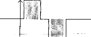
Nous simulons des électrodes cassées (C1 0-10%, C2 25-35%, C3 45-55%, C4 70-80%, C5 90-100%), ce qui provoque une lacune dans le spectre acoustique transmis (fréquences les plus aiguës pour Cl, fréquences les plus grave pour C5) (figure 24).
1 5 10 15
CO =3=eeWM=Wea'n'en=ea=
Cl Z=BM=MR=M=IM=
C2 =M=R=Z=D=De
C3 Z=B=M=M=Wa=nea=
C4 Aile11411.1.1111141114114:=Cinalizi
C5 ceieii=a111111111.1111afflee[3=D=
Figure 24 : Simulation de l'électrode cassée.
La mesure de l'intelligibilité est mesurée 14 fois, dont 3 avec le réglage d'origine et 11 avec un réglage modifié.
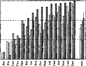
La figure 25, représente les variations du pourcentage de reconnaissance phonétique en fonction des différentes conditions expérimentales. Afin d'évaluer la diminution de l'intelligibilité, nous avons effectué une comparaison de pourcentage entre les performances de chaque réglage dégradé et celles obtenues avec le réglage d'origine.
· Réglage normal
m Réglage modifié
·
|
D) C |
100 80 60 40 20 100 80 |
|
;'12. 60 |
|
|
D) |
|
|
'Tg 40 C |
|
|
20 |
|
D1 02 03
Réglage
*** *** ***
9 |
Al A2 A3
Réglage
· Réglage normal O Réglage modifié
·
** *** * **
100 80 - 60
·
40 -
20 -
Cl C2 C3 C4 C5
Réglage
Figure 25 : Performances moyennes
des 8 sujets implantés en fonction du type de réglage
utilisé :
modification de la dynamique (Haut), répartition
fréquentielle (milieu),
simulation d'électrodes cassées
(bas).
Les trois types d'altération de réglages réalisés mettent en évidence l'importance de différents paramètres de réglage sur la reconnaissance : respect de la dynamique , du nombre d'électrodes actives, de l'intégrité fréquentielle du signal.
1- Modification de la dynamique électrique
Nous avons une dégradation de l'intelligibilité dans les trois cas, mais elle n'est statistiquement significative que pour la première condition. Une distorsion de la dynamique électrique du réglage influe donc sur la compréhension, surtout si le niveau de sonie moyen est inférieur (condition D1, p<0.05) ou supérieur (condition D3, p<0.1) à la normale.
2- Réduction du nombre d'électrode
Une modification de la répartition fréquentielle dégrade considérablement l'intelligibilité (p<0.001) dans les trois cas. Ceci montre que le recodage via l'implant cochléaire des informations fréquentielles demande au patient un temps d'adaptation. La répartition fréquentielle d'un réglage ne doit pas être modifiée trop fréquemment.
3- Simulation d'électrodes cassées
La perte d'information acoustique simulée par mise à zéro de quelques électrodes détériore la reconnaissance phonétique quelque soit leur position (Cl p<0.05, C2 p<0.01, C3 p<0.001, C4 p<p<0.05, C5 p<0.01). Cela montre qu'il est impératif de contrôler la fonctionnalité de toutes les électrodes. Cela peut parfois être difficile chez les enfants implantés cochléaires mais une approximation du réglage peut comme le montre la figure 25 (partie du bas) dégrader fortement la compréhension et donc induire un retard dans le développement du langage chez de l'enfant.
Conclusion
Le principe de fonctionnement de l'implant cochléaire et plus particulièrement celui de l'implant cochléaire Digisonic® impose une grande rigueur dans la qualité des réglages. L'utilisation d'un programme de réglage très ouvert permet, via des techniques psycho-physiques, d'adapter pour chaque sujet, l'information traitée et envoyée.
La reconnaissance de la parole est primordiale pour les sujets implantés cochléaires. Les contraintes étiologiques, anatomiques et psychologiques sont certainement des facteurs déterminants pour les performances de chaque sujet. D'autres paramètres, tels que l'adaptation de la stimulation et du traitement du signal aux spécificités du patient vont permettre d'obtenir le maximum de compréhension admissible par le sujet.
L'objectif de cette partie est d'évaluer par différents tests les effets du traitement du signal et du codage effectué par l'implant cochléaire (en particulier le Digisonic®) sur la reconnaissance de la parole.
Il Le Digigram®
Afin d'analyser au mieux le traitement effectué par l'implant cochléaire, MXM a développé un outil, le Digigram®, qui permet de recueillir les informations transmises de la partie externe à la partie interne de l'implant (figure 26). Cette technique présente l'avantage d'utiliser toute la chaîne de traitement de l'implant cochléaire, du microphone contenu dans le contour l'oreille, à l'antenne émettrice. Toute distorsion engendrée par un de ces éléments sera donc prise en compte. L'activité de chaque canal au cours du temps représentée tel un sonagramme est appelé électrodogramme. Cette mise en forme permet d'analyser le traitement effectué par l'implant cochléaire pour un réglage donné en le confrontant au signal acoustique non traité (figure 26).
a
o.
01101111110,11»,
|
3 |
.11:11.111:11111111.:illit0.111... d1111101111111111111111 ,u nu piliitilLutul: I 0.300 0:400 0.500 0.600 |
|||
|
0.100 0.200 |
0:700 0.000 0.'900 |
|||
Figure 26 Exemple d'un
électrodogramme effectué par le Digigrane Le signal acoustique,
représenté
en bas correspond au mot 'duc'. L'activité
de chaque canal (1 à 15) est représentée en fonction
du
temps, la longueur du trait correspond à la durée de
l'impulsion en ps.
III Importance de l'information contenue dans la stimulation
Plusieurs paramètres contenus dans le signal sonore influencent sur la reconnaissance de la parole. L'information fréquentielle codée par le numéro d'électrode semble être la plus pertinente pour l'implant cochléaire (Friesen et a1,1999). L'enveloppe temporelle qui correspond aux fluctuations de l'énergie en fonction du temps est aussi très informative (Shannon et al, 1995).
Il nous a paru intéressant d'évaluer dans quelle mesure l'information fréquentielle transmise par l'implant cochléaire est intelligible par un ordinateur et d'étudier l'apport de l'enveloppe du signal. Dans un deuxième temps on s'est intéressé à l'importance de chacun de ces paramètres pour la compréhension des sujets implantés cochléaires.
a/ Reconnaissance automatique des voyelles via l'implant cochléaire
L'objectif de cette étude est de comparer deux modèles de reconnaissance de voyelle par ordinateur :
- Le premier modèle utilise toutes les informations envoyées à travers l'implant au cours du temps. L'information tonotopique (numéro d'électrode) et l'information énergétique (énergie de l'électrode stimulée).
- Le second modèle ne tient compte que des informations tonotopiques (numéro d'électrode stimulée) en fonction du temps (l'énergie est de 0 si l'électrode est inactive et 1 si elle est stimulée).
La chaîne de mesure
Le processeur utilisé dans cette étude est un multipeak de la société Cochlear. Il est composé de 20 canaux répartis de 50 à 5500 Hz. Le Digigram est utilisé pour acquérir les signaux envoyés par la partie externe de l'implant cochléaire.
tenue
|
MPeak |
Digigram |
PC
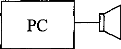
Figure 27: Principe d'acquisition de signaux par le Digigram® via le processeur Mpeak® de Cochlear
Le matériel phonétique :
La quasi-stationnarité des voyelles est intéressante car elle simplifie les calculs (il suffit d'étudier une moyenne temporelle plutôt qu'une analyse temps-fréquence comme cela aurait été le cas avec les consonnes).
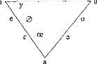
- 4 voyelles /ai, /i/, /u/, /3/ sont utilisées pour l'expérimentation. Elles correspondent respectivement, dans leur représentation formantique, aux trois sommets du triangle vocalique et à la voyelle neutre (cf Figure 8).
Les locuteurs
- 6 locuteurs (3 femmes et 3 hommes) ont prononcé 24 fois chacun des voyelles dans un ordre aléatoire (96 items par locuteur). Afin d'obtenir des voyelles en contexte, chacune d'elles sont contenues dans la phrase «c'est» voyelle «à ça».
- Chaque phrase est numérisée sur ordinateur (16 bits à 44.1 kHz), segmentée pour extraire les voyelles, puis restituée à l'implant via un haut parleur de bonne qualité situé à 30 cm du microphone à une intensité d'environ 70 dB SPL.
- 2 listes sont extraitent : une liste d'apprentissage, une liste de reconnaissance (12 prononciations par voyelle et par liste).
Acquisition et prétraitement
Chaque voyelle est enregistrée via l'implant cochléaire par le Digigram®. Pour chaque acquisition et pour chaque canal, on procède à un moyennage de l'énergie d'une vingtaine de trames (on peut le faire car les voyelles sont des signaux quasi stationnaires). Pour le premier modèle, cela correspond à une moyenne de l'énergie transmise. Pour le deuxième modèle, cela correspond au pourcentage d'activation du canal (car l'énergie a pour valeur 0 ou 1). Pour chaque voyelle on obtient un vecteur à 20 dimensions correspondant aux 20 canaux. Afin de pouvoir comparer les deux modèles on normalise les
vecteurs. 20
18 111Modèle 1
16
· Modèle 2 14 12 10
8
11
Figure 28: Exemple de vecteurs normalisés représentant la voyelle le/ pour les deux modèles.
Reconnaissance des voyelles
Le principe de la reconnaissance est de déterminer par la liste d'apprentissage la voyelle théorique de laquelle se rapproche le plus la voyelle à reconnaître. Pour cela, il suffit de calculer la distance euclidienne entre la voyelle à reconnaître et le barycentre de chacun des groupes de voyelles de la liste d'apprentissage. La plus petite distance correspond à celle de la voyelle la plus probable.
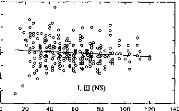
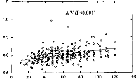
Le pourcentage de reconnaissance entre les quatre voyelles est
supérieur à 90 % pour les deux
modèles (cf tableau I).
Une comparaison de pourcentage ne trouve pas de différence statistique
entre
les performances des deux modèles étudiés
(p=0.90, p=0.93 avec n=288). L'énergie de stimulation de
chaque électrode ne semble pas apporter d'informations supplémentaires pour la reconnaissance de ces 4 voyelles.
Modèle tonotopie + énergie
|
/a/ |
/3/ |
/i/ |
/u/ |
|
|
/a/ |
0.85 |
0.07 |
0.00 |
0.00 |
|
/3/ |
0.15 |
0.85 |
0.01 |
0.01 |
|
/V |
0.00 |
0.01 |
0.91 |
0.00 |
|
/u/ |
0.00 |
0.07 |
0.08 |
0.99 |
0.90
Modèle tonotopie sans énergie
|
/a/ |
/3/ |
/i/ |
/u/ |
|
|
/a/ |
0.89 |
0.03 |
0.01 |
0.00 |
|
131 |
0.11 |
0.93 |
0.01 |
0.03 |
|
/i/ |
0.00 |
0.04 |
0.92 |
0.00 |
|
/u/ |
0.00 |
0.00 |
0.06 |
0.97 |
0.93
Tableau I: Matrice de confusion
entre les 4 voyelles testées pour les deux modèles
utilisés
(n= 288 par modèle).
Distance statistique entre deux populations de voyelles A et B
Nous avons calculé la distance statistique entre les différentes populations de voyelles (24 items par groupe et par locuteur) les pourcentages de reconnaissance étant proches de 100 %, une comparaison de pourcentages semble insuffisante pour dissocier les deux modèles étudiés.
La formule de la distance statistique entre deux populations A et B est la suivante
(o-,, + ol,)
i IM A - M BI D(21,B)=
|
Distances |
énergie + |
tonotopie |
|
131-/u/ |
22.80 |
26.46 |
|
/i/-/a/ |
23.63 |
22.74 |
|
Ii/-131 |
18.59 |
17.35 |
|
131-/a/ |
13.75 |
13.56 |
|
/i/-/u/ |
25.13 |
26.73 |
|
/a/-/u/ |
30.10 |
33.41 |
|
Moyenne |
22.33 |
23.38 |
Tableau II: Distances
statistiques entre chaque population de voyelles deux à deux,
pour
les deux modèles étudiés.
Tout comme les matrices de confusion, les distances statistiques des groupes de voyelles ne différent pas statistiquement en fonction du modèle étudié. L'énergie ne semble donc pas apporter d'informations supplémentaires.
Faut-il pour autant négliger l'enveloppe du signal envoyé par l'implant ? Est-ce que tous les implantés n'utilisent que l'information tonotopique pour la reconnaissance des voyelles?
b/ Modèle de compréhension
An Otol Rhinol Laryngol 1995, sup.166,104: 9,2, 351-353
L'objectif de cette étude est de modéliser, en utilisant la logique flou, la reconnaissance des voyelles /a/, /i/, /u/, /3/ de 4 sujets porteurs d'un implant cochléaire Nucleus de Cochlear. Différents modèles de reconnaissance n'utilisant qu'une partie de l'information transmise au patient via l'implant cochléaire sont expérimentés (255 modèles).
10 locuteurs (5 hommes et 5 femmes) ont été enregistrés. 48 items par locuteur ont été prononcés. Chaque item est présenté en parallèle au sujet implanté cochléaire et via l'implant cochléaire à une carte d'acquisition permettant la reconnaissance par ordinateur.
Pour chaque patient, une comparaison entre la matrice de confusion et celle trouvée par ordinateur détermine le meilleur modèle caractérisant sa reconnaissance.
Les résultats montrent que le modèle représentant le mieux la compréhension varie selon le patient. Certains sujets utilisent la tonotopie, d'autres n'utilisent que l'énergie.
Il est donc tout aussi important pour certain sujet de préserver l'enveloppe temporelle du signal que l'information fréquentielle.
ANALYTIC IMPORTANCE OF THE CODING FEATURES FOR THE DISCRIMINATION OF VOWELS IN THE COCHLEAR IMPLANT SIGNAL
C. BERGER-VACHON, MD, PIO; S. GALLEGO, MS; A. MORGON, MD; E. TRUY, MD
From the Department of Otorhinoleryngology, Edouard I Terriot Hospital, Lyon, France.
The présent study considers the analytic importance of the excitation pulse features delivered by a Nucleus cochlear implant using the FOF 1 F2 strategy. Four cochlear implant patients and 10 speakers uttering two 48-item lists constructed from four basic French vowels participatcd in this study. Patterns were presented to the patients and played at the input of an acquisition system in order to record the pulse features. Confusion matrices obtained with the patients and with automatic recognition procedures were then compared in order to find out the best-matching models simulating the patients' performances, out of 255 possibilitics. The automatic recognition was carried out according to fuzzy logic based on the elementary features of the pulses coding the vowels. Results show that the essential features strongly depended on the subject.
INTRODUCTION
Coding of the acoustic signal by means of a cochlear implant (CI) is still under discussion.1 While several strategies have bcen used, results based only on cl inical performances do not show with enough precision what elementary features are important in the coding for speech recognition. Basically, the stratégies commonly used in a multichannel CI involve the phonetic aspect of language (Nucleus),2 the use of a spectrum (Digisonic),3 and the analog splitting up of energy such as the one produced by Symbion.4 Another step takes place in experiments in which the signal is artificially modified and presented to the patient in order to establish whether or not changes in the coding are significant.5-7
Preliminary experiments have shown that on some pa-
Duration (D) Duration (D)
Amplitude
(A)
Ne
·
Charge C=AxD
Fig I. Structure and parameters of stimulating pulse on any given electrode (E, in text).
) )
tients, vowels with high energy are not confused with lowenergy vowels, even when their frequency configuration is similar. For example, the high energy of the French vowel /a/ makes it quite easy to recognize. The question that emcrged from this finding is the following: "What characteristics in the signal coded by the speech processor allow for the acoustic distinction by the patient?"
Computer simulation allows the testing of a large number of combinations of elementary signal features with the help of models for determining the most important features for the patient. The study presented here aims to find out what is
TABLE 1. MOST LIKELY VALUES FOR FEATURES ESTABLISIIED
DURING
LEARNING STAGE (CORRESPONDING TO ONE
SPEAKER AND ONE PATIENT)
|
/a/ |
li/ |
lu/ |
le/ |
|
|
El |
19 |
21 |
21 |
20 |
|
E2 |
16 |
9 |
18 |
16 |
|
Al |
11 |
22 |
26 |
5 |
|
A2 |
24 |
11 |
20 |
13 |
|
Dl |
26 |
7 |
8 |
24 |
|
D2 |
17 |
29 |
6 |
15 |
|
Cl |
29 |
4 |
4 |
26 |
|
C2 |
27 |
30 |
2 |
25 |
Units are artificiel numbers calculated from confusion matrix.
|
Magnetic |
CI |
Acquisitior |
Desktop |
|
|
Tape |
_ Speech |
-- Storage |
||
|
Recorder |
Processor |
Caïd |
Computer |
|
Fig 2. Block diagrarn of acquisition system.
important in the coding that allows distinction between vowels. Some work already done by the Melbourne team8 established that the second formant (F2) and the F1F2 representation were important in the patient's recognition process. This testing could be extended by using theoretic models. A more analytic study of the features of the stimulation pulse is also possible. Models can be created to evaluate the contribution of each feature of those elements that play a role in the distinction perceived by the patient. This is the aim of our work.
PA VENTS
The four patients who collaborated in this work all used the Nucleus 22 cochlear implant, and the Mini Speech Processor (MSP) programmed with the FOF1F2 strategy and in the bipolar plus one mode. They were two women, one man, and a young girl. The FOF1F2 strategy was chosen in order to limit the number of features studied in this experiment.
The man (CO), 46 years of age, had all his electrodes working. He became deaf at the age of 41. He had 20 channels active and was a star patient. The first woman (BA), 40 years of age, also had all her electrodes working and 20 channels active. Deafness occurred at the age of 2. The second woman (LA), 32 ycars old, had an ossificd cochlea with only 5 channels active (15 to 20; 18 was nonfunctioning). She became deaf at the age of 28. The girl (AM), 12 years old, had 19 channels active (channel 7 was closed). She was close to being a star patient. Deafness occurred at the age of 9.
In all four cases, the channels covered the frequency range from 280 Hz to 4 kHz; two fifths were in the Fl range (280 to 800 Hz) and the others were in the F2-F3 range (800 to 4,000 Hz). The band-pass filter was distributed according to a logarithmic scale.
ACOUSTIC MATERIAL
Speakers. Ten staff members, five men and Pive women, collaborated in ibis work by reading the acoustic material. They were from 20 to 30 years old and had clear voices. Two lists were read by each speaker, the first for learning and the second for recognition.
Vowels. Four French non-nasal vowels were chosen. They were situated at the points and in the middle of the vowel triangle in the F1F2 space.
Classic values for their formants are vowel F1 300 Hz
and F2 2,000 Hz; vowel /u/, F1300 Hz and F2 800 Hz; vowel F1 650 Hz and F2 1,250 Hz; and vowel /e/, F1 500 Hz and F2 1,500 Hz.
These vowels were well separated in the F1F2 space. Each vowel was embedded in a sentence: "c'est /v/ ça," with /v/ standing for the vowel. Each vowel was repeated 12 times at random to produce two 48-vowel lists.
VOWEL RECOGNITION
Patient. Each patient was asked to recognize the vowels spoken by each speaker. Confusion matrices were then estab-
Second
Dl C2 A2 Dl
C2E1 AIC1 Al E2 A2D2
C2E1E2 Cl DI D2 A2E1E2 C2D1D2
A2C1C2D2 AI A2C I D2 AIEIE2D1 AICIDID2
TABLE 2. FIRST AND SECOND BEST-MATCHING MODELS Patient First
Single (I feature)
AM Cl
BA Cl
CO E2
LA D2
Pair (2 features)
AM ClE1
BA CID1
CO El E2
LA C1D1
Triplet (3 features)
AM CIE1E2
BA A2C2D2
CO A1E1E2
LA A2DID2
Quadruplet (4 features)
AM A2C1E1D2
BA A 1 A2E1E2
CO A 1A2EIE2
LA A2C1D1D2
lished. The patient first listened to the training list in order to adapt his or her discriminating possibilitics. Then, for each utterance of the recognition list, he or she was asked to give his or her best choice for the vowel. A confusion rnatrix was constructed for each speaker and for each patient, leading to a total of 40 matrices.
Computer. A previous study9 showed that fuzzy logic, close to a probabilistic dccision, was well adapted to simulate the patient's recognition of the vowels. Let us in troduce this method by supposing that k features are studied for each vowel. The recognition process can be broken into two stages. During the learning stage, a table is filled out which records, for each value of the feature, the number of occurrences corresponding to each class. Ranges have been normal ized from 1 to 32 for each item, and only integer values were taken. In each box of this table, there is a histogram showing the occurrence of the 32 values. This histogram was established in order to indicate the "probability" of each of the 32 values. The CI mapping was adapted to each patient and a table constructed for each implantce and each speaker. Consequently, a full table contains 32 (values) x 4 (vowels) x 8 (features) = 1,024 numbcrs.
The features are dcscribed in the electrode number (E), the amplitude (A), the duration (D), and the charge (C) (Fig 1). An example of the most likely values, for each feature and for each vowel, is given in Table 1.
At the recognition stage, an "unknown" pattern "x" needed to be classified. This pattern was represented by eight values (one for each feature). For each feature, a score was attributed to each class. This score was obtained from Table 1. The sum of the scores was calculated for each vowel and x was classitied to the closest vowel (having the highest sum). When all the vowels of the recognition list were classified, a confusion matrix was established characterizing the automatic recognition.
Score of Model. A Hamming distance was constructed between the confusion matrix observed with the patient, and the confusion matrix of the automatic recognition (each automatic recognition corresponded to a model). The sum of the absolute values of the difference, calculated box by box between the two matrices, gave us the score of the model.
PARAMETERS
Signal Acquisition. The signal corning from the speech processor was fed into a computer. In order to keep the same signal (for the patients and for the automatic recognition), the lists were recorded on a high-fidelity Revox tape recorder. The signal, transformed by the processor, was taken by an acquisition card designed for this tank. The processor was set according to the patient's map values. The system worked under the control of the computer. Last, data were kept on disks (Fig 2).
It should be kept in mind that for each stimulating pulse, representing a formant, the Nucleus device delivers six elementary pulses bearing the information of the electrical stimulation. Out of these six elementary-pulse sets, it is possible to extract the features of the stimulating pulse (Fig 1): E, A,
D, and C. Positive and negative phases have the same duration.
Set of Features. To facilitate the analytic study, the Nucleus system was used according to the simple FOF1F2 strategy, and only the information on the voice formants was considered. For each pitch period during the utterance of a vowel, the Nucleus delivers two stimulating pulses (one foreach formant) containing the following information (eight features): El E2
A 1 A2 D 1 D2 Cl C2, with 1 and 2 referring to the pulse. Thus, 255 recognition spaces can bc constructed with these features. Each space (corresponding to a model) has a base that combines these eight features according to the combinative analysis.
RESULTS
As the aim of the work is to cstimate which features arc likely to bc used by CI subjects in the recognition process, a set of features received a high score when its confusion matrix was close to the confusion given by the patient ("bestmatching" model). Models were ranked according to this proximity. Results are given in Table 2 averaging the 10 speakers. Thcy are grouped according to the number of features.
DISCUSSION
Results showed that the recognition given by the models with a single parameter did not always put the tonotopic information of the second formant (E2) in top best-matching position. When two parameters were used, the ElE2 combination was not systematically the bcst. Three times out of four, the best-matching model was based on the first formant properties only (number and energy).
When a third parameter was added, best-matching models took information mostly from the two formants. It is worth noting that thebest matching mode I changedfrom one patient to another. The settings of a speech processor should take into account the patient's recognition strategy in some way. This is now possible with the present CI versatility.
Schematically, we suggest the following interpretation of the patients' results. For the star patient, CO, the results corresponded to the tonotopic representation. For patient BA (prelingual deafness), the first formant was mostly used, and the patient did not take full advantage of the tonotopic representation. Patient LA, with only a small number of electrodes, made excellent use of the information given by the charge. Patient AM (good performer) had a tendency to take data from Fl and F2, which was not specifically the electrode position.
It could be interesting in the future to generate the pulses on a speech processor simulator, and to test directly, with the patients, the best combinations given by the models.
CONCLUSION
This work considers, through the use of models, the importance of some features of the stimulating pulse of a Nucleus speech processor. This was done with CI patients using a corpus of four French vowels. The main results can be summarized thus. The second formant position was not always the best strategy for making the distinction. Data on the first formant (including the charge) were also important. The classic phonetics model E1E2 was not always the bestmatching model. Again, data on the energy turncd out to be equa]ly important. Relevant features differed from one patient to another, suggesting that a strategy should be adapted to each subject. These results need to be confirmed by testing in direct stimulation with the patients.
ACKNOWIF_DGME,;TS -- The authors thank people and
institutions that supporter/ thcir u
·ork: the Civil Hospitals of Lyon,
the French Council for Research, the Rhône-Alpes Region, the API company,
the University of Lyon, and Professor L. Collet from the Edouard Herriot
Hospital.
REFERENCES
1. Wilson BS, Finley CC, FarmerlC, Lawson DT. Comparative studies of speech stratégies for cochlear implant. Laryngoscope 1988;98:1039-97.
2. Clark GM,Blamey PJ, Brown AM, et al. The University of Melbourne Nucleus multi-electrode cochlear implant (monograph). Adv Otorhinolaryngol 1987;38:1-190.
3. Belieff M, Dubus P, Leveau JM, Repetto JC, Vincent P. Sound processing and stimulation coding of the Digisonic DX10 15-channel cochlear implant. In: Hochmair-Desoyer IJ, Ilochmair ES, eds. Advances in cochlear implants. Vienna, Austria: Manz, 1994:198-203.
4. Eddington DK. Speech recognition in deaf subjects with multichannel intracochlear electrodes. Ann NY Acad Sci 1983;83:241-58.
5. Berger-Vachon C, Collet L, Djedou B, Morgon A. Model for understanding the influence of some parameters in cochlear implantation. Ann Otol Rhinol Laryngol 1992;101:42-5.
6. Dillier N, WaiKong L, Hans B. A high spectral transmission coding strategy for multi-electrode cochlear implant. In: Hochmair-Desoyer II, Hochmair ES, eds. Advances in cochlear implants. Vienna, Austria: Manz, 1994:152-7.
7. Doering WH, Schneider L. Electrical vs. acoustical speech patterns of German phonemes using the Nucleus CI-system. In: Fraysse B, ed. Cochlear implant, acquisition and controversies. Toulouse, France: Service ORL, 1989:243-53.
8. Blamey PJ, Clark GM. Place coding of vowels formants for cochlear implant patients. J Acoust Soc Am 1990;88:667-73.
9. Gallego S, Perrin E, Berger-Vachon C, Collet L, Truy E. Recognition of vowels by cochlear implant using a fuzzy logic, Int. AMSE Modelling & Simulation Conference, Lyon, France, July 4-6, 1994. AMSE Press, 1994;9:103-16.
15
9 iNI(8 )1131(7
Sur le système Digisonic, il est possible d'activer l'ensemble des canaux du sujet implanté à chaque trame de stimulation. L'objectif est de montrer qu'une partie des informations peut être inutile, voire même perturbante pour la discrimination phonétique.
al Extraction de pics
A chaque trame de stimulation, l'implant cochléaire Digisonic® peut activer de 1 à 15 électrodes. Le choix du nombre maximum de canaux ouverts par trame ne sert qu'à ajuster la sensation de sonie (plus le nombre de canaux ouverts est important, plus le niveau de sonie est élevé).
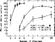
L'objectif de cette partie est d'étudier l'effet du nombre de canaux activés sur la reconnaissance. Stimuler seulement x canaux sur quinze, ceux correspondant aux plus grandes énergies de la trame, équivaut à extraire l'information émergente du signal.

Figure 29 : Exemple du principe d'extraction de pics (5 pics par cycle)
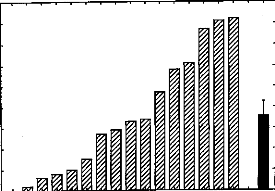
Nous avons comparé les distances statistiques entre différents groupes de voyelles (/a/, /i/, /u/, /3/). Le protocole expérimental est très proche des études II/a/ et II/b/. 10 locuteurs (5 hommes et 5 femmes) ont prononcé 24 fois chaque voyelle (en contexte «c'est» voyelle «à ça») dans un ordre aléatoire. Chaque voyelle est transmise, via un haut parleur, à l'implant cochléaire Digisonic®. L'implant cochléaire a une répartition fréquentielle en échelle Bark (Calliope, 1989) et est en mode 'N' avec 15 canaux actifs par trame. La carte d'acquisition du Digigram®, connectée à la sortie de l'antenne de l'implant, numérise et enregistre sur PC chaque voyelle. Le PC génère 15 fichiers différents par voyelle
segmentée. Ils correspondent à une simulation du mode 'N' avec 1 à 15 canaux actifs par trame. La figure 30 illustre un exemple des modifications de l'électrodogramme induite par le nombre de canaux par trame.
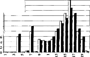
Chaque voyelle est décomposée en un vecteur à 15 dimensions correspondant chacune à une moyenne en énergie de 20 trames. Dans chaque condition, la distance statistique entre les voyelles est mesurée. Les résultats montrent que la séparation des différentes voyelles dépend du nombre de canaux actifs par trame et des voyelles à séparer. Deux canaux actifs par trame correspondent au réglage le plus efficace en moyenne pour séparer au mieux les groupes de voyelles. Les distances statistiques se dégradent lorsque l'on utilise trop de canaux actifs par trame.
|
Canaux |
/a/-/i/ |
la/-/u/ |
la/-131 |
/i/-/u/ |
/u/-131 |
/i/-131 |
Moyenne |
|
1 |
7.7 |
11.0 |
8.0 |
6.2 |
8.5 |
78.7 |
13.6 |
|
2 |
24.9 |
32.8 |
9.5 |
14.7 |
7.5 |
31.8 |
17.9 |
|
3 |
11.9 |
14.5 |
9.5 |
19.1 |
8.8 |
41.6 |
14.8 |
|
4 |
10.1. |
12.4 |
9.3 |
12.8 |
9.2 |
54.0 |
14.1 |
|
5 |
13.7 |
11.8 |
8.7 |
11.8 |
12.0 |
34.2 |
13.8 |
|
6 |
12.4 |
9.5 |
7.8 |
13.5 |
10.9 |
49.4 |
13.7 |
|
7 |
14.0 |
10.9 |
6.1 |
15.1 |
7.0 |
32.1 |
12.0 |
|
8 |
16.2 |
12.5 |
6.7 |
14.8 |
6.3 |
26.8 |
12.4 |
|
9 |
15.4 |
12.8 |
6.7 |
14.3 |
6.3 |
25.1 |
11.9 |
|
10 |
15.3 |
13.2 |
6.4 |
14.0 |
6.3 |
24.3 |
11.7 |
|
11 |
15.4 |
14.1 |
6.6 |
14.0 |
6.4 |
24.0 |
11.9 |
|
12 |
15.7 |
14.4 |
6.6 |
14.0 |
6.4 |
24.0 |
12.0 |
|
13 |
15.9 |
14.4 |
6.6 |
14.0 |
6.4 |
24.0 |
12.0 |
|
14 |
16.0 |
14.5 |
6.5 |
14.0 |
6.4 |
24.0 |
12.0 |
|
15 |
16.0 |
14.5 |
6.5 |
14.0 |
6.4 |
24.0 |
12.0 |
Tableau Ill: Distances
statistiques en fonction du nombre de canaux actifs
et du couple de voyelles
à séparer.
· -111-1.1 -111111111111111111111111111111111111111111111111111111 111111111 III .111111.
·
III 111111111111111111111
Il 11 11
· Hutii 11..1 11111111111111111111111111111111111111111111111111111101111111111111HiiIIIH-............-............---
· I 11111111111111111111 .111 111-111.-1111- III 111 1
·. 1111111111111111111111111--
-11.-111-111 1111111
·.11. 1111111111111111111111111111,-.1....... -11
·· .11 11111111 I
··
· .111.11 1.111 1111 11111 1111111111 1111 111. 1111 11111 1111 11111
·III III' I
·· -111mill 111t.111..1...1111111111111111111111111111111111111111111111111111111111111111111111111111111111111.
· -111-1111-11 111-11-111111111111111111111-11111.11111111-1111 1111-111111111111111111111111-111 1111111111-.1111111 1
·10
· ..11i11 11.11-1--111-111-11111-1--111-...11111-.111.1111 111. 1111 .11111111. 111--11
...11111111111111111111111111111111111111,111..1111111111111111-11111111111111111111111111111111111111111 111111111-1111-1111.11.....--
111111111 in 1111.11111111111111111111111111111111111111.....--
.....111.-111 .1111 Illii-11111.1111110
·.n0.11111111-
Figure 30: Electrodogramme d'un /3/ avec 1 (gauche), 2 (milieu), 5 (droit) canaux actifs par trame.
b/ Rehaussement spectral
Les résultats précédents montrent que 2 canaux actifs par trame correspondent à la meilleure séparation des voyelles. Pour le patient implanté, cela ne semble pas exploitable car avec ce type de stimulation, la sonie est faible et la voix, par la pauvreté de l'information, n'est pas 'naturelle' et semble saccadée.
Afin d'augmenter le nombre de canaux actifs et d'améliorer le rapport signal sur bruit, nous avons voulu étudier les avantages d'une technique de rehaussement spectral.
Rehaussement spectral
Afin de faire ressortir les pics d'énergie de certains canaux, on utilise un algorithme qui va atténuer les canaux adjacents des maxima. Le nombre de maxima étudiés est de 1 à 15, l'atténuation de 0 à 95% par pas de 5 %. 300 configurations de réglage sont donc envisagées. Un exemple figure 31, permet de mieux comprendre ce principe de rehaussement.
I
Figure 31: Exemple de rehaussement. Signal d'origine (Gauche);
Atténuation de 20 % avec 3 Maxima (droite).Tout comme l'étude sur l'extraction de pics, nous utilisons les voyelles /a/, /i/, /u/, /3/ prononcées 24 fois chacune par 10 locuteurs, puis segmentées et modifiées par le PC via l'implant cochléaire Digisonic® et le Digigram®. Les distances statistiques entre chaque couple de voyelles sont ensuite calculées pour toutes les configurations (300 simulations de réglages différents).
Le tableau IV, est un résumé des résultats (2100 distances statistiques calculées). Seules les meilleures configurations y sont représentées.
|
|
|
|
||
|
|
|
|
||
|
|
|
|
||
|
|
|
|
||
|
|
|
|
||
|
|
|
|
||
|
|
|
|
||
|
|
|
|||
Tableau IV: Meilleures distances statistiques en fonction des voyelles,
du nombre de maxima et de l'atténuationLes distances statistiques indiquées dans le tableau IV sont plus grandes que celles obtenues avec la technique d'extraction de pics, ce qui indique une meilleure différentiation entre les voyelles concernées. De plus le nombre de maxima choisis est compatible avec le confort du sujet implanté (niveau de sonie et fluidité de la voix perçue par le patient). Ce type de traitement semble donc intéressant à étudier pour la discrimination des voyelles chez le sujet implanté cochléaire.
Pour évaluer de manière objective l'intelligibilité du signal émis à la partie interne de l'implant cochléaire Digisonic, trois types de reconnaissance ont été effectués. Dans un premier temps nous avons évalué la reconnaissance obtenue par ordinateur. Celle-ci n'a qu'une valeur indicative sur l'intelligibilité maximale que l'on peut avoir, puisque le mode de reconnaissance des phonèmes est très éloigné de celui pratiqué par les sujets implantés cochléaires. En second lieu, nous avons mesuré l'intelligibilité du signal de l'implant cochléaire obtenu chez des normo-entendants et des surdités moyennes en restituant par un algorithme, le signal de manière acoustique. Pour finir, nous avons mesuré l'intelligibilité obtenue chez des sujets implantés cochléaires.
al Reconnaissance des voyelles par analyse discriminante
Avant de mesurer les performances du sujet implanté cochléaire, il est intéressant d'estimer l'intelligibilité du signal émis par l'implant cochléaire. Pour ce faire nous avons évalué par analyse discriminante (Rouanet et le Roux, 1993), la séparation et le pourcentage de discrimination d'un échantillon de 4 voyelles, puis des 16 voyelles de la langue française (cf figure 8).
Une première étude (C. Berger-Vachon, et al, 1997) a eu quatre objectifs.
1- développer une technique de reconnaissance par une analyse discriminante (test plus performant que la mesure de distance euclidienne),
2- évaluer la séparation et la discrimination des voyelles /a/, /i/, /u/, /3/ via l'implant cochléaire Digisonic®,
3- comparer les données obtenues dans les 2 modes de l'implant cochléaire le mode 'A' - i.e. mode parole - (avec au maximum 6 canaux ouverts par cycle) et en mode 'N' - i.e. mode musique - (avec au maximum 15 canaux ouverts par cycle),
4- comparer les performances effectuées par le traitement de l'implant cochléaire à celles obtenues par un modèle d'implant simulé sur PC.
Les résultats montrent une grande efficacité de l'analyse discriminante dans la classification des voyelles /a/, /i/, /u/, /3/. Le mode 'A' semble être le plus efficace mais il n'est pas significativement différent du mode 'N' et du simulateur d'implant. Les conclusions sont peu affirmatives car le nombre de locuteur est faible (2) et les pourcentages de reconnaissance très proche de 100.
J.C. Bera, S. Gallégo, L Collet, C.
Berger-Vachon
Advances in Modeling & Analysis, 1999, in press
L'objectif de cette étude a été d'évaluer les séparations d'une population plus importante de voyelles que l'étude précédante (les 16 voyelles de la langue française) via l'implant cochléaire Digisonic® et un modèle simulant l'implant cochléaire.
L'analyse des résultats montrent de très grands pouvoirs discriminants des différentes populations de voyelles (0.94 à 1.00). La classification par un modèle basé sur la FFT est identique voire moins bonne que celle de l'implant Digisonic®.
Le traitement effectué par l'implant apporte donc suffisamment d'informations pour permettre de différencier toutes les voyelles de la langue française par une analyse discriminante.
Vowel Processing Through a Cochlear Implant
A Model
of Speech Coding
J.C. Bera *, S. Gallego **, L. Collet***, C. Bergpr-Vachon***
* Acoustic Centre, Ecole Centrale de Lyon, 69131 Ecully-CEDEX
(France)
**MXM Laboratories, 06224 Vallauris-CEDEX (France)
***Laboratory
« Perception and Auditory Mechanisms »,
ORL Dpt, E. Herriot
Hospital, 69437 Lyon CEDEX 03 (France)
Abstract
The construction of an efficient code for deaf people fitted with a Cochlear Implant (CI) is still an op cri problem.
Classically, a spectrum analysis of the acoustical signal is ma :'e and periodieally distributed at the end- of the auditory nerve of a patient. Clinically, this approach has been widely used by the physicians Also, analytical considerations need to be made on the acoustic signal.
In this paper, the results obtained with the discrimination of the French vowels taken at the output of a CI are discussed and compared with a FFT analysis (CI &FFT are two models). Vowels are well separated, two by two, by a discriminant analysis... even those which were expected to be close, using both strategies. The discussion indicates that the eigenvalues or the distances used to assess the separation may not be a very relevant item to simulate the human behaviour in this situation because they separate vowels which are similar to the ear.
Further studies need to be carried out in order to understand
better the phenomenon.
Key-words: Cochlear implants, Signal
processing, Mathematical strategies, Confusion matrices
Paper presented, and selected, at CCM'98 (Contribution of Cognition to Modelling), International AMSE-Conference, Lyon-France, 6-8 July 1998.
1.Introduction
The recognition of speech by human beings has raised a lot of questions [1,2]. Many models have been established and most of the strategies start with a frequency-time representation of the signal, which is further processed [3,4,5].
This approach is widely accepted for the ear. In the inner ear, it is admitted that the cochlea performs a tonotopic decomposition of the acoustic signal which is distributed at the ends of the auditory nerve. Then, complex mechanisms occur, starting at the brainstem, to end up into an interpretation finally given by the brain.
In the case of totally deaf people, the cochlea is non-functional and it breaks the auditory chain. To beat this handicap, a cochlear implant is surgically introduced and electrodes are put in the cochlear duct. Then, electrical pulses are delivered according to a signal analysis performed by an external device called the speech processor [6].
Mos6 of the studies conducted with patients point out that in difficult situations, the results stay below 70% [7,8,9]. In the experiments the stimulus is embedded in standard contexts such as «hvd» for vowels (where v stands for the vowel) and «aCa» for consonants (where C indicates the consonant). Most of these studies have deepiy analysed die situation with the patient, but suffer of a lack of consideration from the signal processing point of view.
For instance, it is well known that the patient's background has a tremendous influence on his ability to perform die recognition and use efficiently his prosthesis. The evolution with time of die recognition scores has to be taken into account. At die end, it turns out that a deeper look into die intrinsic properties of the signal should bring interesting considerations on what is to be expected from die patient. For instance, it is difficult to imagine that if two stimuli are similar, the patient would separate them in a nonsense context. But, the similarity is something which is not obvious to be defined «mathematically speaking». This is why we will take two approaches to evaluate the distance between «elementary» phonemes.
An objective assessment of the signal processing can be done directly, and compared to the classical FFT analysis.
In the language, vowels are supposed to be stationary and their structure can be represented by a stable vector giving, with its co-ordinates, the distribution of energy in die spectrum. This is a very easy way to see the signal and interesting to make objective studies on the signal.
The questions which are raised in this work are:
- what is the efficiency of the coding of the French vowels by the French cochlear implant (Digisonic DX-10 of MXM) relatively to the classical coding, obtained in the same conditions, with a FFT analysis?
-what is the performance of both systems when vowels, perceptually close, are taken?
- what is the signification of the confusion when human behaviour is considered?
Basically, CI and FFT lead to models of the language. These models are based on the knowledge on speech, in perception and on acoustical properties.
Acoustical analyses will be developed further in this text.
2.Material and methods
2.1 Cochlear implant use
Basically it can be considered that the acoustic wave undergoes the transformations indicated in figure 1, from the acoustic wave to the brain.
Brain Interpretation
|
Outer & Middle Ear |
Inner |
Auditory Pathways |
|||
|
Ear |
|||||
Acoustical Signal
Figure 1: Classical stages in hearing.
Outer and middle ears transfer the acoustical vibrations to the inner ear.
In the inner ear, vibrations are converted into electrical stimuli which enter the auditory pathways.
The auditory pathways carry the influx to the brain, and some transformations occur at this stage, mostly in the detection of basic features (temporal and energy) in the signal.
In the brain, important and mysterious transformations take place. Generally it is considered that the features are « printed » in the temporal cortex, then matched with patterns already known by the subject, and finally interpreted according to his background and knowledge of the situation.
In the inner ear there is the organ of Corti which performs the transformation from acoustical vibrations into electrical stimulus. When this organ is totally non functioning (in both ears) the chain is broken, leading to a deep cophosis, and the subject is completely deaf.
In order to beat this handicap, scientists have developed cochlear implants intended to replace this deficient function.
The schematic structure of a cochlear implant is shown on figure 2. The description given is the DX 10 system of the French firm MXM, which was used in this work.
Skin
Micro
Antenna 0
Speech processor
Antenna
Detection & distribution
Electrodes
Figure 2: The main two parts of a cochlear implant.
In the speech processor, the signal is sampled at a 15.6 kHz rate, and a numerical analysis takes place. A FFT is performed and 64 spectrum lins are calculated and grouped into 15 frequency bands ranging (table I) from 122 to 6558 hertz (Hz). Then 15 pulses with a fixed amplitude are constructed. The duration of each pulse is proportional to the energy of the corresponding frequency band. The pulses modulate a 3 MHz carrier which is transmitted, through the skin, to the implanted part of the device.
After reception, the implanted electronic device demodulates the carrier and distributes, sequentially, to 15 electrodes the electrical energy contained in the pulses. According to their
place in the cochlea, the electrodes represent different frequencies... and the brain must deal with them and «guess» the content of the message formulated by the speaker.
|
Band |
Frequency range |
|
1 |
122-244 |
|
2 |
244-366 |
|
3 |
366-488 |
|
4 |
488-610 |
|
5 |
610-732 |
|
6 |
732-854 |
|
7 |
854-976 |
|
8 |
976-1098 |
|
9 |
1098-1342 |
|
10 |
1342-1708 |
|
11 |
1708-2196 |
|
12 |
2196-2806 |
|
13 |
2806-3660 |
|
14 |
3660-4880 |
|
15 |
4880-6588 |
Table I: Distribution of the frequency bands (given in Hz) of the Digisonic DX-10 cochlear implant.
2.2 Acoustical material
Twelve French vowels were taken in the following context:
« c'est /v/ ça » (it is /v/ that)
where /v/ stands for the vowel. Vowels are written in phonetic notation and indicated between slashes (table II). The use of a context is intended to minimise the « side effects » (coarticulation influence).
Two French speakers (male and female) participated in the experiment. They were in their mid-twenties.
Bach-vowel was uttered 10 times leacling to 10 samples for each clans:
|
Phonetic symbol |
Typical word |
Category |
|
/a/ |
Pute (paw) |
O |
|
/a/ |
Pâte (pasta) |
O |
|
/à/ |
dans (in) |
N |
|
/e/ |
...té (summer) |
O |
|
/ce/ |
beurre (butter) |
O |
|
/8/ |
baie (bay) |
0 |
|
/0/ |
le (the) |
O |
|
/i/ |
fille (girl) |
O |
|
lo/ |
porte (door) |
O |
|
/o/ |
beau (beautiful) |
O |
|
/I/ |
feu (lire) |
O |
|
/o/ |
bon (good) |
N |
|
/u/ |
sol (money) |
O |
|
/y/ |
brûler (to burn) |
O |
|
Ice I |
brun |
N |
|
IÈ/ |
brin (blade) |
N |
Table II: French vowels used in this text; the category (Oral or Nasal) is indicated in the right column
2.3 Signal recording
The diagram of the system used to record the signal is indicated on figure 3. The acoustical signal was sampled at a 16 kHz rate by a classical 16-bit sound-blaster card, using the corresponding routines in the Windows package.
The microphone was a low-pass filter (cut-off frequency was 8 kHz) and it had also the antialiasing function. Then the signal was segmented on disc files in order to select only the vowels to be studied.
In nasal phonemes, the air uses the nasal track. When phonemes are oral, the nasal track is closed.
Windows routines
Sound blaster
^-> Personal computer
Disc
storage
Micro 0--
Figure 3: Block diagram indicating the recording of the phonetic material.
2.4 FFT analysis
The FFT analysis was performed on data stored in the computer. An overlap of 50% occurred between two consecutive windows. Samples were weighted according to the Hamming formula. The duration of the analysis window (frame) was 128 points corresponding to 8 milliseconds (ms) of signal.
Sixty-four spectrum fines were calculated and arranged according to the 15 frequency bands of the Digisonic (table I).
On each utterance, 19 frames with a 50% overlap have been taken in the middle of the vowel. Each frame led to a 15-dimensional vector, where each component contained the energy of a frequency band. The final values, for a band and for an utterance, were the average of the energies calculated on the 19 frames.
2.5 Pulses recording
The Digisonic performs a spectrum analysis of the speech signal, and the FFT parameters indicated in section 2.4 were taken for comparison purposes.
A pulse, representing the energy, was associated to each band.
Pulses were automatically recorded using a special device (Digistim) supplied by the manufacturer (figure 4).
The acoustical material to be analysed, previously recorded in the computer, was played at the input of the Digistim (device supplied by MXM) and the duration of the pulses (and the time
between two pulses) were detected and then stored into the computer. This work was done under the control of a special software developed by the manufacturer.
Sound Blaster
Desktop Computer
o
Cochlear Implant
Digistim MXM
|
Loud speaker |
Microphone |
Figure 4: Recording of the pulses.
2.6 Discriminant analysis
The discriminant analysis is a classical linear method of classification [10]. Only two-class comparisons were performed in this study. With the 16 classes (one class for each vowel), we had 16* 15/2 =120 comparisons.
Classically, the overlap between two classes is measured by X the eigenvalue of the T-1E matrix, where:
T is the matrix of total covariance,
E is the covariance matrix of the centres of gravity of the classes.
It can be proved [11] that X belongs to the [0,1] range in the 2-class case.
The largest eigenvalue was taken to assess the separation of the classes. Let us remind that X =0 is a « perfect » confusion and X =1 is a « perfect » separation.
In order to make more sensible comparisons, the separation of
each pair of two classes has been also indicated, in projection on the main
eigenvector associated to the largest eigenvalue.
The results given by the
classical statistical formula (given below) have been shown:
- in
S'ab = a b
0. a2 cr 2b
where ma and mb are the means for each class a and b and 6a2 and o the corresponding variances.
3 Results and discussion
Results obtained with the female voice are given (tables III and IV). Those obtained with the male voice are equivalent.
|
/a/ |
/a/ |
/a/ |
/o/ |
/e/ |
/s/ |
/I/ |
/i/ |
[É/ |
/o/ |
h/ /ce/ |
/6/ |
/u/ |
/y/ |
/êe' / |
||
|
/a/ |
**** |
07.2 |
03.7 |
08.2 |
09.3 |
08.9 |
16.1 |
10.0 |
09.1 |
12.8 |
06.5 |
10.1 |
08.3 |
07.8 |
07.3 |
08.2 |
|
/a/ |
0.95 |
**** |
15.9 |
09.6 |
13.3 |
19.8 |
11.9 |
16.1 |
07.1 |
13.4 |
08.1 |
11.8 |
15.6 |
12.4 |
07.7 |
09.9 |
|
/à/ |
0.99 |
0.98 |
**** |
08.9 |
10.6 |
12.4 |
05.7 |
12.4 |
08.7 |
04.3 |
09.1 |
16.8 |
10.9 |
09.5 |
08.2 |
09.2 |
|
/o/ |
0.99 |
0.99 |
0.96 |
**** |
09.3 |
09.0 |
09.4 |
11.3 |
05.3 |
12.9 |
07.2 |
07.2 |
09.0 |
08.9 |
07.5 |
08.3 |
|
/e/ |
0.99 |
0.9 |
0.99 |
0.99 |
**** |
07.4 |
06.4 |
12.8 |
05.7 |
10.7 |
06.1 |
08.9 |
08.6 |
08.6 |
08.6 |
06.6 |
|
/d |
0.99 |
0.99 |
0.97 |
0.99 |
0.99 |
**** |
05.3 |
10.1 |
09.0 |
07.1 |
12.8 |
08.4 |
07.7 |
07.3 |
15.8 |
07.2 |
|
/I/ |
0.99 |
1.00 |
0.98 |
0.97 |
1.00 |
0.96 |
**** |
09.7 |
11.7 |
05.4 |
08.3 |
07.5 |
06.6 |
06.3 |
08.6 |
06.3 |
|
/i/ |
1.00 |
1.00 |
0.99 |
0.99 |
0.99 |
1.00 |
0.99 |
**** |
14.3 |
09.0 |
13.8 |
08.6 |
10.6 |
05.3 |
12.0 |
03.7 |
|
re |
0.96 |
0.97 |
0.99 |
0.98 |
0.99 |
0.99 |
0.99 |
0.99 |
**** |
12.2 |
06.7 |
11.1 |
12.3 |
12.6 |
05.1 |
11.0 |
|
/o/ |
1.00 |
0.99 |
0.97 |
0.99 |
0.98 |
0.99 |
0.97 |
1.00 |
0.99 |
**** |
08.8 |
07.6 |
05.6 |
05.4 |
08.4 |
06.2 |
|
/o/ |
0.99 |
0.99 |
0.98 |
0.96 |
0.99 |
0.97 |
0.96 |
0.99 |
0.99 |
1.00 |
**** |
08.0 |
11.4 |
10.3 |
05.4 |
09.0 |
|
/ce/ |
0.99 |
1.00 |
0.99 |
0.99 |
0.99 |
0.99 |
0.99 |
1.00 |
0.99 |
1.00 |
1.00 |
**** |
06.2 |
07.0 |
09.1 |
07.4 |
|
/6/ |
1.00 |
1.00 |
1.00 |
0.99 |
1.00 |
0.99 |
0.99 |
1.00 |
0.99 |
0.95 |
0.99 |
0.99 |
**** |
08.0 |
09.1 |
08.1 |
|
/u/ |
1.00 |
1.00 |
0.99 |
0.99 |
0.99 |
0.99 |
1.00 |
0.97 |
1.00 |
0.99 |
0.99 |
0.97 |
0.99 |
**** |
08.1 |
03.0 |
|
/y/ |
1.00 |
0.99 |
0.99 |
0.96 |
1.00 |
0.98 |
1.00 |
1.00 |
0.99 |
0.99 |
0.99 |
1.00 |
0.98 |
0.99 |
**** |
08.8 |
|
/Ce/ |
1.00 |
1.00 |
0.99 |
0.99 |
0.99 |
0.99 |
0.99 |
0.97 |
1.00 |
0.99 |
1.00 |
0.99 |
0.99 |
0.92 |
1.00 |
**** |
Table III : Separation between the vowels using the FFT; Xs are on the bottom left and Sabs on the top right.
Results were calculated with the FFT model and with the cochlear implant coding. 2,s are indicated on the bottom left and Sabs on the top right of the tables. It can be seen that the vowels
were well separated in all the situations. Both models (FFT and Implants) of vowel representations behaved equally.
Then, it was expected that some vowels would have a high overlap. This is the case for /Ce/ and /V which are not easy to distinguish by normal listeners in usual speech. In our example, the automatic separation is almost perfect.
|
/a / |
/a/ |
/à |
/ /o / /e/ |
/s/ |
/I/ |
/i/ |
/"Ê / /o/ bo / /ce/ /ô/ |
/u/ |
/y/ |
/Ce/ |
||||||
|
/a / |
**** |
15.0 |
08.4 |
13.9 |
10.9 |
19.7 |
06.7 |
18.6 |
13.6 |
06.8 |
10.9 |
17.6 |
14.7 |
12.2 |
20.1 |
14.8 |
|
/a/ |
1.00 |
**** |
14.9 |
05.4 |
29.2 |
15.8 |
11.7 |
29.4 |
07.9 |
24.0 |
09.3 |
11.7 |
33.4 |
26.1 |
24 6 |
08.8 |
|
lij / |
1.00 |
0.99 |
**** |
14.2 |
14.4 |
12.1 |
07.1 |
22.2 |
08.7 |
05.1 |
16.0 |
10.9 |
07.5 |
13.0 |
17.4 |
08.1 |
|
/a / |
0.99 |
0.98 |
0.99 |
**** |
20.5 |
10.2 |
11.2 |
19.9 |
05.2 |
28.1 |
12.5 |
05.7 |
19.6 |
18.2 |
17.3 |
06.1 |
|
/e/ |
0.99 |
1.00 |
0.99 |
1.00 |
**** |
13.2 |
13.3 |
11.0 |
11.2 |
09.2 |
15.5 |
11.3 |
04.0 |
06.5 |
09.3 |
20.5 |
|
/s/ |
0.99 |
0.99 |
0.99 |
0.99 |
1.00 |
**** |
06.8 |
18.3 |
07.2 |
18.1 |
15.4 |
10.7 |
15.4 |
13.8 |
11.8 |
18.8 |
|
/V |
0.99 |
0.99 |
0.99 |
0.99 |
0.99 |
0.96 |
**** |
22.0 |
06.8 |
04.2 |
08.7 |
08.3 |
16.7 |
14.7 |
17.3 |
08.3 |
|
/i/ |
1.00 |
1.00 |
1.00 |
1.00 |
0.97 |
1.00 |
1.00 |
**** |
22.3 |
19.8 |
23.9 |
11.8 |
13.1 |
05.8 |
07.2 |
25.4 |
|
ft' / |
1.00 |
0.99 |
0.99 |
0.95 |
1.00 |
0.98 |
0.97 |
1.00 |
**** |
10.2 |
07.0 |
04.2 |
12.8 |
17.6 |
18.0 |
04.7 |
|
/o/ |
1.00 |
1.00 |
0.97 |
1.00 |
1.00 |
0.99 |
0.96 |
1.00 |
0.97 |
**** |
09.6 |
15.3 |
07.2 |
11.6 |
19.3 |
13.8 |
|
bo / |
0.99 |
0.98 |
0.99 |
0.99 |
1.00 |
0.99 |
0.99 |
1.00 |
0.97 |
0.98 |
**** |
11.4 |
14.0 |
17.4 |
19.0 |
05.2 |
|
le / |
1.00 |
0.99 |
0.99 |
0.98 |
0.99 |
0.99 |
0.98 |
0.99 |
0.97 |
0.98 |
0.98 |
**** |
11.7 |
11.1 |
09.9 |
08.4 |
|
/5/ |
0.99 |
1.00 |
1.00 |
1.00 |
0.97 |
1.00 |
1.00 |
0.97 |
1.00 |
0.99 |
1.00 |
1.00 |
**** |
07.5 |
12.0 |
18.5 |
|
/u/ |
0.98 |
1.00 |
0.99 |
0.99 |
0.98 |
0.99 |
1.00 |
0.95 |
1.00 |
0.99 |
0.99 |
0.99 |
0.95 |
**** |
05.4 |
17.3 |
|
/y/ |
1.00 |
1.00 |
0.99 |
1.00 |
0.98 |
0.98 |
0.99 |
0.94 |
1.00 |
1.00 |
0.98 |
0.98 |
0.98 |
0.95 |
**** |
16.0 |
|
/Ce/ |
1.00 |
1.00 |
0.99 |
1.00 |
0.99 |
0.99 |
0.99 |
1.00 |
0.93 |
0.99 |
0.94 |
0.99 |
1.00 |
1.00 |
0.99 |
**** |
Table IV: Separation using the cochlear implant. Considering these results two comments can be made:
1) The vowels were carefully spoken in good signal to noise ratio conditions (soundproof room); it would be interesting to see the results in more « natural » (noisy) situations.
Comparisons were made on the voice of one speaker only... in the case of several speakers, it would be useful to reconsider the situation.
2) The representation which was taken (vectors and eigenvalues in a discriminant analysis)
did not appear to be a good model of human behaviour with the vowels. People are more used to cope with the variability which is included in normal speech conditions.
Further studies are needed, in order to investigate deeper that matter. For instance, a look at the structure of the representative vectors cannot be avoided. A model of human behaviour in such conditions is still to be made and the spectral distribution presented in this work must be improved to match better human psycho-acoustical performances.
IV Conclusion
Vowels representation by a cochlear implant, using the model of a spectrum vector and a discriminant analysis (or a statistical distance), is very efficient to separate the vowels.
This efficiency was surprisingly high because several vowels (acoustical objects) which are similar perceptually were perfectly separated.
Results given by a FFT analysis were very similar to those obtained with a cochlear implant.
This work indicates that further studies are needed to set up a model more adapted to human behaviour.
Acknowledgements
The authors acknowledge the participation in this experiment of the students involved in the project: M. Doutiaux, S. Faucher, B. Fuselier, E. Laribe, D. Rousseau.
References
[1] Fant R. « Auditory patterns of speech », W. Dunn edit., Cambridge, M.I.T. Press, (1967), 111-125.
[2] Roberts L. « Speech and brain mechanisms », Princeton Univ. Press, (1959).
[3] Berger-Vachon C., Gallego S., Bera J.C.,.Arnoux E., Vissac C. «A Model of vowels representation using a cochlear implant », Advances in Intelligent Systems, 526-532 Ed. F.C. Morabito, I. 0 . S . Press, Amsterdam , (1997)
[4] Perkell J., Klatt D.H. « Invariance and invariability in speech processes », Lawrence Earlbaum, Hullsdale N.J., USA, (1983).
[5] Serniclaes W., De Guchteneere R., Secqueville T., Bachelot G., Genin J., Meyer B., Chouard C.H. « Objective evaluation of vowel identification with the Digisonic cochlear implant », Audiology, 35, 23-36 (1996).
[6] Belaieff M., Dubus P., Leveau J.M., Repetto J.C., Vincent P. « Sound processing and stimulation coding of Digisonic DX-10 15-channel implant », Advances in cochlear implantation, Ed I.J. Hochmair (Innsbruck), 198-203 (1996).
[7] Robinson K., Summerfield A. « Adult auditory learning and training », Ear & Hearing, 51S- 65S (1996).
[8] Dorman M.F., Loizou P.C. « The identification of consonants and vowels by cochlear implant patients », Ear & Hearing, 162-166 (1998).
[9] Skimmer M.W. et al « Speech recognition at stimulated soft, conversational and raised to loud vocal efforts by adults with cochlear implants », J. Acoust. Soc. Am., 101, 3766-3782 (1997).
[10] Sebestyen G.S. « Decision making processes in Pattern recognition », Mc Millan (1962).
[11] Lebard L., Morineau A., Fénelon J.P. « Traitement des données statistiques », Dunod-Paris (1982).
b/ Restitution acoustique des signaux provenant de l'électrodogramme
Précédemment, nous avons montré que l'information résultant de l'implant cochléaire Digisonic® est très pertinente. La question maintenant posée est de savoir si la manière dont l'information est transmise au système auditif nécessite un recodage. En effet, l'information, très pertinente pour l'ordinateur, peut être mal décryptée par les voies auditives.
Il nous a paru intéressant de simuler le signal entendu par les sujets implantés cochléaires, par une restitution acoustique des électrodogrammes, afin d'évaluer son intelligibilité lors d'un traitement normal via les voies auditives.
Cahier de l'audition, 1998, 10:6, 22-24
L'objectif de cet article est de mesurer l'intelligibilité du signal traité par l'implant mais restitué de manière acoustique. 10 sujets normo-entendants et 20 sujets atteints d'une surdité moyenne ont participé à l'expérimentation. Afin d'étudier les processus naturels du traitement auditif, il n'y a eu aucun entraînement de décryptage du signal émis.
La reconnaissance phonétique moyenne (liste de 34 mots tri-phonémiques de Lafon) est de 86% pour les normo-entendants (allant de 80 à 95 % selon les sujets) et de 45% pour le groupe de personnes atteintes de surdités moyennes (allant de 0 à 85 % selon les sujets).
L'information transmise par l'implant cochléaire est intelligible et décryptée de manière naturelle par le système auditif. Par contre elle est beaucoup moins riche que l'information non traitée et nécessite une attention plus grande.
SIMULATION ACOUSTiQUE
DU MESSAGE DÉLiVRÉ PAR
L'IMPLANT COCHLÉAIRE
DiGISONIC DE iviXivi
Les performances des sujets porteurs d'un implant cochléaire sont très supérieures, à surdité équivalente, à celles des sujets utilisant une aide auditive classique. Ceci suggère que l'appauvrissement du signal effectué par l'implant pourrait être bénéfique à l'intelligibilité. Il est de deux ordres :
· Appauvrissement fréquentiel
· Appauvrissement temporel
Notre étude a consisté à simuler les "appauvrissements" effectués par l'implant et à réaliser des tests sur normo-entendants et sur malentendants.
Il est important de noter que le signal résultant ne peut en aucun cas être strictement comparé à ce qu'un implanté cochléaire perçoit. Le but est ici d'évaluer l'effet du codage.
Subjects using cochlear implant have far better performances that conventional hearing aided subjects having the same hearing loss. This suggest that temporal and spectral impoverishments performed by the implant could be beneficial to intelligibility.
:Our study consists in simulating these impoverishments in order to measure "their effect on normal-hearing and hearing-impaired subjects' intelligibility.
|
||||||||
|
||||||||
Contour
d'oreilleAntenne
externePC
Electrodes implantées
Récepteur
interne
internePatient
Digigram
Simulateur
Figure 1 Synoptique du Digisonic DX10 de MXM
Stéphane Garnier
Doctorant Boursier du Groupe d'Audioprothésiste ENTENDRE, UPR CNRS 5020, Lyon
Stéphane Gallego
Doctorant Boursier de la Société MXM, UPR CNRS 5020, Lyon
Angélique Veive
Etudiante en audioprothèse Lyon
Lionel Collet
Professeur à l'Université Lyon 1 Directeur du laboratoire "Neurosciences et Systèmes Sensoriels", UPR CNRS 5020, Lyon
Figure 2 Principe du traitement du signal
F FT (Digisonic NIX.1)
Sommation des sinusoïdes
L'analyse fréquentielle effectuée par le processeur se fait sur 128 points à la fréquence d'échantillonnage de 15,6 kHz. Les 64 bandes d'énergie ainsi obtenues sont alors regroupées en 15 bandes ajustables en fonction du réglage du patient. Les informations sont encodées et envoyées à travers la peau. Le décodeur interne interprète le message et transmet un courant proportionnel à l'énergie de chaque bande à l'électrode qui lui correspond. Le rythme de stimulation peut être fixe (entre 100 et 400 Hz) ou proportionnel à la fréquence fondamentale de la voix mesurée en temps réel.
correspondante). Un algorithme de superposition et sommation (overlap and add) a été mis en oeuvre pour assurer la continuité du signal. La figure 2 illustre l'ensemble du traitement, la partie gauche est réalisée par le processeur de l'implant, la partie droite par le simulateur.
4. Population
L'étude porte sur 10 sujets normo-entendants et sur 20 sujets malentendants ayant tous une surdité équivalente.
5. Déroulement du test
Les sujets sont dans une chambre insonorisée. Le test consiste à leur faire écouter une liste de mots (listes de Lafon) ayant été préalablement traitées par l'implant et reconstituées par la méthode décrite ci-dessus.
Le score ainsi obtenu est comparé à celui du même test sans traitement. Les sujets normo-entendants ont été testés à 40 dB SPL et les sujets malentendants à 60 dB SPL.
Deux modes de fonctionnement sont disponibles. Le mode "musique" permet de stimuler l'ensemble des électrodes, c'est à dire que toutes les informations énergétiques sont transmises.
En mode "parole", seules les 6 bandes fréquentielles de plus grande énergie sont utilisées.
2. Le DIGIGRAM
o
4 o
o Non traitée
· Traitée
t
tes \tis èee
k6e-t-te
Figure 3 Scores d'intelligibilité des deux populations dans les deux conditions
|
|
100 90 80 70 60 50 40 30 20 10 |
Le DIGIGRAM est un système qui permet de récupérer en temps réel les informations transmises par le processeur en se substituant à la partie interne de l'implant (Beliaeff et al. 1994). C'est un outil indispensable à toute étude basée sur l'analyse des données transmises à l'implant.
3. Reconstruction du signal acoustique
Les blocs de données, recueillis par le DIGIGRAM, sont composés de l'énergie de stimulation de chaque électrode en fonction du temps.
Pour chaque bande de fréquence (i.e. chaque électrode), nous avons synthétisé une sinusoïde centrée dans cette bande à laquelle nous avons attribué l'énergie mesurée par le DIGIGRAM. Cette somme de sinusoïdes représente une fenêtre de notre signal (de durée égale à celle de la trame de stimulation
RÉSULTATS
Les résultats d'intelligibilité des deux populations dans les deux conditions d'écoute sont représentés sur la figure 3.
On remarque que le traitement affecte très peu l'intelligibilité des normo-entendants alors que celle des malentendants est très fortement réduite.
Nous pouvons nous intéresser à la corrélation entre l'intelligibilité du signal traité et celle du signal non traité, celle-ci est représentée sur la figure 4. On constate l'existence d'une forte corrélation entre ces deux grandeurs :
(r = 0.855, p < 0.001).
70-
·
·
Figure 5 Corrélation entre la perte
d'intelligibilité due
au traitement et l'intelligibilité de la
voix normale
E
ez: -
Le.

|
|
|
|
|||
|
|
|||||
. s
· '
·
·
·
· . .
·
·8
· 000 0 0
o
·
60
50 -
a)40 40 -
·
',moi_: 30 -
;120-
-(7) 10 -
Ç
· Malentendants 'a 0 -
a) o Normo-entendants
' '
40 50 6 '
60 70 80 90 100
Intelligibilité de la voix normale(%)
0-10 o-
100
· Malentendants 90 o Normo-entendants80 70 60 50 40 30 20 10 o
0 10 20 30 40 50 60 70 80 90 100 Intelligibilité de la voix normale (%)
Figure 4 Corrélation entre les scores d'intelligibilité
de la voix traitée et non traitéeDe la même façon, la perte d'intelligibilité due au traitement est significativement liée à l'intelligibilité de la voix normale
(Fig. 5 ; r = -0.539, p = 0.002).
DISCUSSION
Lorsque le sujet malentendant
connaît déjà des difficultés avec
la voix normale, celles-ci sembleot être amplifiées lorsque l'on applique le traitement.
La diminution plus rapide de l'intelligibilité de la voix traitée peut être expliquée par une plus forte implication des fonctions psychoacoustiques élémentaires (résolution temporelle et/ou fréquentielle).
Les différentes composantes du signal traitées sont résolues chez le normo-entendant, ce qui lui permet d'analyser correctement le signal.
Chez le malentendant, certaines composantes peuvent être non résolues, le signal devient alors impossible à analyser de façon fine.
CONCLUSIONS
Les résultats de cette étude appuient l'hypothèse que les meilleures performances des sujets porteurs d'un implant cochléaire seraient dues à la restauration (même grossière) du codage fréquentiel par la place. La prothèse auditive pour le sourd profond doit tendre vers la correction ou le remplacement du codage fréquentiel déficient.
D
|
||
Les Cahiers de i Auddon - VoL 10 - N16 - Nov./0éc 97
Le traitement effectué par l'implant cochléaire et restitué acoustiquement est intelligible en situation de calme. Nous avons voulu mesurer ce qu'il en était avec un signal de parole bruité, qui représente une
stimulation plus réelle.
Advances in Modeling & Analysis, 1997, 37: 37-44
Dans cet article nous mesurons l'intelligibilité du signal traité par l'implant et restitué acoustiquement sur un signal de parole bruité à différents rapports signal sur bruit (non bruité, S/B -3 dB, S/B +3 dB). Afin d'étudier l'intérêt de la méthode d'extraction de pics pour réduire le S/B, les deux modes de l'implant cochléaire sont testés ('A' et 'N').
Les résultats ne montrent pas de différences entre les modes 'A' et 'N' sur l'intelligibilité. Plus le bruit est important plus la reconnaissance phonétique est faible. La compréhension dans le bruit reste très bonne ; avec un bruit 1.4 fois plus grand en énergie que le signal on obtient encore 35 à 40 % de reconnaissance correcte.
Simulation of an hearing aid based on cochlear implant coding
Stéphane Garnier 1'2, Stéphane Gallego 1'3, Véronique Ziempfer 1, Christian Berger-Vachon 1
« Perception and Auditory Mechanisms » Laboratory, UPRESA CNRS 5020, Pav. U, E. Herriot Hospital, 69437 Lyon Cedex 03, France
2 ENTENDRE Hearing Aids Dispensers Group, GIPA 2, 40 route du Pontel, 78760 JouarsPontchartrain, France
3 MX1VILaboratory, les Mimosas, Quartier Croix Rouge, 06600 Antibes, France.
SUMMARY
Cochlear implant coding strategy has already shown the great ability of the auditory system to adapt to temporal and spectral impoverishment. The aim of this study is to simulate the signal processing made by cochlear implant to evaluate a possible application to conventional hearing aids. The system which was used to extract stimulations characteristics is the processor of the MXM DIGISONIC DX10 transcutaneous multichannel cochlear implant. Reconstruction of the acoustic signal has been performed using informations given by the implant. Eight normal-hearing subjects participated to the study. The test consisted in a vocal audiometry with three signal to noise ratios (silence, -3 dB and 3 dB). Results show that when noise is present, the processing has a negative effect on the intelligibility. In the other hand, good results were obtained in silence. They are rather interesting for a possible application of such a coding to the conventional correction of severe hearing loss.
KEYWORDS : Hearing aids; Cochlear implant; Simulation
INTRODUCTION
Hearing in noise is the highest source of discomfort for people with a sensorineural hearing loss. Then, hearing comfort and intelligibility in noise should be an important aim of hearing
aids. Nowadays, analogic technologies are the most commonly used, but they cannot implement complex algorithms to reduce interfering noise before amplification. For example we could mention the adaptive filtering which adjusts the frequency gain response regarding background noise, or directional microphones selecting the information at the source. To be implemented in hearing aids, these techniques meet the limitation of analogic technology. Apparition of numeric systems, allowing a more powerful signal processing, is encouraging.
Cochlear implant (CI) coding strategy has already shown the high ability of the auditory system to adapt to temporal and spectral impoverishment. The implant used in this study (DIGSONIC DX10 of MXM) extracts the energy out of 15 frequency bands and transmits an electrical stimulation to the implanted electrodes along the cochlea. Energy is proportional to the corresponding frequency band. In general, only the bands of greatest energy are transmitted.
The aim of this study is to imitate the signal processing used in cochlear implant in order to judge its possible application to conventional hearing aids. In order to do so, we evaluated in simulation the effect of this processing on normal-hearing subjects. Results obtained using that « smearing » of the signal are presented below.
METHODS
Information coding with a cochlear implant
Cochlear implant is classically used with post-lingually totally deaf aduits or with prelingually totally deaf children.
In accordance with the spectral tonotopy of the cochlea, each electrode of the implant stimulates a specific nerve bundle representing a frequency bandwidth. But the auditory sensation of implanted patients cannot be fully compared to a normal one. Practically, electrodes are disposed in the first round of the cochlea. Then they stimulate mostly the basal part which corresponds to frequencies ranging from 1 kHz to 16 kHz (Greenwood 1990). Consequently, there is a transposition of the sensation from low to high frequencies.
The DIGISONIC DX10 manufactured by the MXM Laboratory is a transcutaneous, 15- channel cochlear implant. It is composed of two parts (figure 1), one externat (microphone, digital processor and emitting antenna)- and the other internai (Receptor and implanted electrodes which are distributed chirurgically along the cochlea).
Microphone
Figure 1 : Digisonic DX10 block diagram
The digital processing is based on a real time 128-point Fast Fourier Transformation (FFT). The 64 lines of the spectrum are gathered into 15 adjustable frequency bands. Each band is allocated to an electrode. Encoded information is sent through the skin to the internai receptor. The internai decoder transmits to each electrode an intensity which is proportional to the measured energy in its frequency band. The stimulation rhythm can be fixed (100 to 400 Hz) or proportional to the measured fondamental frequency of the voice.
Two distinct working modes are available. The « music » mode allows the stimulation of ail the electrodes. In the « speech » mode, only 6 bands (at the maximum) which have the highest energy are transmitted.
Clinical results
h is important to recall clinical results of cochlear implanted patients. Mean scores of 12 subjects with the Lafon's lists are reported in figure 2 (Meyer et Al. 1994).
These results support the present study. They show that cochlear implanted persons (thus having a total cophosis) have better results than people with profound hearing loss using an acoustical hearing aid.
|
||||||||
|
||||||||
Figure 2 : Mean results of 12 Digisonic cochlear implanted subjects (Lafon's lists). In ordinate : 1 month (white), 3 months (gray) and 6 months (black) alter surgery. DIGIGRAM
The DIGIGRAM is a system allowing the real-time recuperation of pulses information transmitted by the processor. It can be substituted to the internai part of the implant (Beliaeff et Al. 1994). A serial link with a Personal Computer (PC) enables the storage of the full information for further processing.
Signal reconstruction (Simulation)
Data blocs collected by the DIGIGRAM show the energy distributed by each electrode along the cochlea and during the time (see figure 3).
Processing has been programmed on a PC 486 DX2 66.
For each frequency band (i.e. each electrode), a sinusoid centered on this band has been synthesized, and the energy measured by the DIGIGRAM has been applied to this pure tone. The summation of these sinusoids defines a "window" of the resulting signal (its duration is equal to a frame of the stimulation). An overlap and add algorithm has been used to insure the signal continuity.
Signal elementary frame Energy
1
2
3
n
4
Electrode number
12
13
14
15
Figure 3 : Digigram information representation
The restitution has been performed directly from the PC to a SoundBlaster card connected t a loudspeaker.
Subjects
The study involved 8 normal-hearing subjects (mean age 22, standard deviation 1.8). All subjects were volunteer students who did not receive any specific training to the task to be done.
Procedure
Subjects were seated in a soundproof room. The test consisted in asking them to listen to a word list (Lafon's cochlear lists) which had been previously treated with the implant processor and with the reconstruction algorithm.
Lafon's cochlear lists are composed of 17 French words containing three phonemes (for a total of 51 phonemes). These lists are commonly used in France for the vocal audiometry.
The number of recognized phonemes gives the intelligibility score of each subject.
The test had been performed in three situations : silence and with two masking noises (signal to noise ratio -3 dB and 3 dB) and for the two modes of the implant (« speech » and « music »). Word lists were different in each one of the six tests. Silence means that the recordings have been made in a sound proof room, with a very high signal to noise ratio.
RESULTS
Figure 4 shows the mean recognition scores calculated over the subjects. They were obtained for each CI working mode and for each signal to noise ratio.
It can be seen that the noise had a strong influence on the recognition percentage.
The good recognition score obtained in silence is" encouraging. The signal smearing involved by the implant like processing led to good results on the subjects' performances, results corresponding to those observed with CI patients.
In addition, this study has been made without any preliminary training. As it can be seen on figure 2, implanted patients have an important delay before reaching their optimal score. It can be hoped that some training could bring better results.
T
100
80
Pourcentage
of recognized 60 phonemes 40
20
Silence S/N=3 dB S/N=-3 dB
Speech Mode Silence S/N=3 dB S/N=-3 dB
Music mode
Figure 4 : Scores obtained for each functioning mode
and for each signal to noise ratioDISCUSSION
Through these results, it is seen that there is a strong information redundancy in speech. Indeed, the drastic selection of the information introduced by the signal processing did not dramatically lower the intelligibility of speech in silence.
Let us consider the possible hypothesis that hearing loss discomfort is partly due to the masking effect induced by the noninformative part of the signal. This is obvious when a noise is present. This masking effect is already present among normal hearing subjects. In hearing
impaired people, the broadening of auditory filters greatly enhances this phenomenon. The larger the auditory filters are, the more disturbing the noise is.
Results are also somewhat surprising. Only the spectral peaks of the signal have been kept, and they are above the noise level (when S/N = 3 dB). In this condition, the noise should not have influence the recognition scores, but this was not the case. Further work is needed to see more deeply that phenomenon.
h can be imagined that the selective action of our signal processing (only 6 pure tones are used in speech mode) can bring some help for peuple with difficulty to separate speech from noise.
CONCLUSION
Used in simulation, the coding strategy of the MXM cochlear implant did not dramatically lower the hearing performances of normally hearing subjects in quiet circumstances. This raises hopes for the application in conventional hearing aids.
Consequently, picking information on the spectrum maxima appears to be a good way of representation of the acoustic signal. Now, it needs to be tested with people with a profound hearing loss, in order to bring a extension of the results obtained with cochlear implanted subjects.
ACKNOWLEDGMENT
This work was supported by a Brant from the ENTENDRE Hearing Aids Dispenser Group. The authors thank also the French National Scientific Research Center (CNRS) and the Hospitals of Lyon.
They also acknowledge the help of professors L. Collet and A. Morgon from the E.N.T. clinic of the Edouard Herriot Hospital of Lyon.
REFERENCES
Beliaeff Michel, Dubus Philippe, Leveau Jean-Marc, Repetto Jean-Claude, Vincent Philippe. (1994) Sound signal processing and stimulation coding of the Digisonic DXJO 15-channel cochlear implant. Advances in Cochlear Implants, edited by I.J. Hochmair-Desoyer and E.S. Hochmair, Innsbruck University, Austria, 198-203.
Bogli Hans, Dillier Norbert (1991) Digital speech processor for the nucleus 22-channel cochlear implant. Annual International Conference- of the IEEE Engineering in Medicine and Biology Society, Prague, May 18-21, 13 (4), 1887-8.
Greenwood DD (1990) A cochlear frequency-position fonction for several species-29 years later. J. Acoust. Soc. Am. 87 (6), 2592-605.
Kompis Martin, Dillier Norbert (1994) Noise reduction for hearing aids : combining directional microphones with adaptive beamformer. J. Acoust. Soc. Am. 96 (3), 1910-3.
Meyer B, Jacquier I, Fugain C, Chouard C-H (1994) Clinical results of the mzdtichannel cochlear implant DIGISONIC. Advances in Cochlear Implants, edited by I.J. HochmairDesoyer and E.S. Hochmair, Innsbruck University, Austria, 198-203.
Les études précédantes ont permis d'évaluer l'efficacité du traitement du signal effectué par l'implant cochléaire Digisonic® dans l'extraction des éléments permettant d'obtenir une bonne séparation des groupes de phonèmes. Nous avons aussi montré que l'information extraite par l'implant pouvait être traitée de la même manière par le système auditif qu'un signal de parole conventionnel.
Cependant, nous ne pouvons en conclure que le traitement du signal de parole effectué par l'implant apporte une bonne intelligibilité chez le sujets porteur de l'implant. Pour cela, seuls les résultats cliniques peuvent nous renseigner. Nous allons comparer les résultats obtenus par les patients à ceux mesurés par ordinateur ou chez les normo-entendants par reconstruction du signal.
Seize sujets porteurs de l'implant cochléaire Digisonic® ont participé à l'expérimentation consistant à évaluer les performances de reconnaissance de la parole. Quatre parmi les seize ont eu une insertion du porte électrode, difficile suite à une cochlée ossifiée (Dur, Fau, Pin, Rob).
a/ Apport de l'implant cochléaire avec ou sans aide de la lecture labiale
Plusieurs tests de reconnaissance ont été effectués. En premier lieu, nous avons voulu estimer l'apport de l'implant cochléaire sur la compréhension de la parole avec ou sans support de la lecture labiale.
Pour chaque sujet, nous avons mesuré le pourcentage de reconnaissance phonétique avec des listes de 34 mots tri-phonémiques proposées par Lafon. Celles-ci ont été prononcées par une orthophoniste dans trois conditions, avec lecture labiale seule, avec implant cochléaire sans lecture labiale, avec implant cochléaire et aide de la lecture labiale. Dans chaque condition, une liste parmi 20 était choisie aléatoirement.
Les résultats sont représentés individuellement figure 32. Les phonèmes sont reconnus en moyenne, à 44% (s.d. 5) avec la lecture labiale seule, 60% (s.d.6) avec l'implant cochléaire sans lecture labiale et à 81% (s.d. 3 %) avec l'implant cochléaire et la lecture labiale. Ces résultats sont comparables avec ceux obtenus sur d'autres types d'implants cochléaires (Tyler et al, 1997).
|
|||
|
|
||
|
|||
|
|||
|
|||
.o
.D C
Q--J-6
C
o
W
u 0 %.
· %. D I-- CO
7;o
41) c.t)
6 C D ta
Ce Ô.Ce le
(..) ta.
Figure 32 Pourcentage de reconnaissance de listes de 34 mots tri-phonémiques pour 16 sujets
porteurs de l'implant cochléaire Digisonice, avec lecture labiale (LL) bâton vide, implant seul (IC) bâton
hachuré , lecture labiale plus implant (LL+IC) bâton quadrillé.
Les résultats sont inhomogènes, mais peuvent être déterminés en partie en fonction des antécédents de chaque sujet porteur de l'implant cochléaire (cochlée ossifiée, durée de privation). L'implant cochléaire apporte statistiquement (par comparaison par rapport à 0) de l'intelligibilité à tous les sujets testés. L'implant cochléaire sans lecture labiale apporte une information supérieure statistiquement (par anova) à la lecture labiale seule (individuellement par comparaison de moyenne LL<IC pour 8/16 sujets, LL>IC pour 1/16 sujets). L'implant cochléaire avec lecture labiale apporte une information supérieure statistiquement (par anova) à l'implant cochléaire seul (individuellement par comparaison de moyenne IC<IC+LL pour 14/16 sujets, LL>IC+LL pour 0/16 sujets). L'apport de la lecture labiale est d'autant plus important que les résultats avec l'implant seul sont faibles (sujets Pin, Fau, Roi).
Si l'on compare les performances obtenues par reconstruction acoustique (puis écoutés par des normoentendants) et celles des meilleurs sujets implantés, on trouve une grande similitude. Les résultats varient au alentour de 90 % de reconnaissance avec des plafonds de 95%. Par contre la reconnaissance par ordinateur a montré des pourcentages très proches de 100%. Cela voudrait dire que l'information envoyée par l'implant cochléaire est suffisante pour reconnaître 100 % des phonèmes, mais que la manière dont elle est codée n'est pas idéale pour le système auditif (5% à 10% des
phonèmes sont mal différenciés).
le La suppléance mentale
La reconnaissance phonétique de non-mots (Doumèche, 1997) ou logatomes est certainement le meilleur moyen chez des sujets porteurs de l'implant cochléaire pour estimer le traitement du signal transmis par les voies auditives. D'autres facteurs, tel que le champ lexical, la mémoire de travail et le temps d'accès au lexique conditionnent aussi les performances du sujet porteur de l'implant cochléaire dans des situations réelles telles qu'une conversation avec une autre personne.
Nous avons voulu étudier l'effet de la suppléance mentale dans la reconnaissance de la parole chez les sujets porteurs d'un implant cochléaire. Pour ce faire nous avons mesuré le pourcentage de reconnaissance phonétique pour trois tests de reconnaissance phonétique différents sans aide de la lecture labiale.
- Le premier test consiste à reconnaître des mots mono-syllabiques. La suppléance mentale n'intervient
pas pour ce type de tache, seuls des éléments phonétiques vont permettre la discrimination,
- Le deuxième test consiste à reconnaître des mots tri-phonémiques ( cf a/). La suppléance mentale joue un rôle limité,
- Le dernier test consiste à reconnaître les phonèmes contenus dans une liste de phrases. La suppléance mentale est ici importante.
Les résultats sont représentés individuellement figure 33. Les phonèmes sont reconnus en moyenne, à 53% (s.d. 6) pour les mots mono-syllabiques, 60% (s.d.6) pour les mots tri-phonémiques et à 70% (s.d. 8) pour les phrases.
Les phonèmes sont statistiquement (anova) mieux reconnus dans les phrases que dans les mots. Les phonèmes sont statistiquement mieux reconnus dans les mots tri-phonémiques que dans les mots mono-syllabiques.
Il existe de fortes corrélations entre les tests (test de Pearson R=0.88 p<0.001 entre les mots monosyllabiques et les mots tri-phonémiques, R=0.85 p<0.001 entre les phrases et les mots monosyllabiques, R=0.87 p<0.001 entre les phrases et les mots tri-phonémiques)
|
100 c c ce% 40 o u aè 20 C .c |
|
·
C D
ti)
C
o
2
V*"' .0 O
·-
· .0
·
· VI O C0 °0 1. 43 u 41e o
U oe --1 0 0 ° 0
Figure 33 : Pourcentage de reconnaissance phonétique sans lecture labiale
pour 16 sujets porteurs de l'implant cochléaire Digisonice, mots mono-syllabiques (bâton vide),
mots tri-phonémiques (bâton hachuré), phrases (bâton quadrillé).La figure 34, représente les corrélations entre les reconnaissances phonétiques de la liste de mots mono-syllabiques et celles des deux autres tests. Il existe une relation linéaire entre les performances à partir des deux listes de mots et une relation non-linéaire entre les performances avec la liste de mots mono-syllabiques et la liste de phrases. La suppléance mentale pourrait expliquer cette non-linéairité. Il suffit d'avoir entre 50 à 60 % de reconnaissance phonétique avec des mots mono-syllabiques pour avoir environ 100 % de reconnaissance phonétique avec des phrases.
100 80 60 40 20
|
|
|
|
|
||
·
·100
aft
80
600
.c
a 40
20
o
0 20 40 60 80 100
Mots mono--syllobiques (%)
|
||
0 20 40 60 80 100
Mots mono--syllobiques (X)
Figure 34 : Relation entre la reconnaissance phonétique avec la liste de mots mono-syllabique et,
la liste de mots tri-phonétiques (gauche), la liste de phrases (droite)
pour les 16 sujets implantés cochléaires.cl Speech tracking
Cette suppléance a un coût. Plus on supplée, plus on doit être attentif et moins l'on peut analyser de mots à la minute. L'objectif de cette partie est, d'étudier le nombre de mots à la minute que peut reconnaître chaque sujet implanté cochléaire par le test de "speech tracking". Nous cherchons également à savoir s'il y a une relation entre le taux maximum de mots analysés et la reconnaissance phonétique.
Les résultats sont représentés individuellement figure 35.
90
80
70"I- 60 o
50
."170 40 o
30
20
10o
C t.) D VI .0 0
·
·
·
·
·
· "" '0 .0 0 C
|
|
||
Figure 35 : Flux moyen de mots (speech tracking) analysés
pour chacun des 16 sujets porteurs de l'implant cochléaire Digisonice:Le débit moyen de mots analysés par le groupe de sujets implantés testés est de 36 mots à la minute (s.d. 29). Il est compris entre 0 et 82 mots/minutes.
Comme l'indique la figure 36, de fortes corrélations existent entre les résultats des tests du "speech tracking" et les résultats des tests de reconnaissance phonétique (test de Pearson R=0.89 p<0.001 entre le speech tracking et les mots mono-syllabiques, R=0.82 p<0.001 entre le speech tracking et les mots tri-phonémiques, R=0.78 p<0.001 entre le speech tracking et les phrases).
,00 100
80
60 60
40 t 40
20
0 0
0 20 40 60 80 100 0 20 40 60 80 100
E
coe,
te
80
20
·
·
·
·
·
··
·
··
·
·
"
·t
· es
·
··
··
·
·Speech trocking (mot/min) Speech tracking (mot/min)
·
·
·
··
·
··
·
·
·
·
·
·
·
·
·20 40 60 80 100 Speech trocking (mot/min)
t 00
ifts
2 80
o
3 60 P.
ô 40
20
o o
Figure 36 : Relation entre le speech tracking et la reconnaissance phonétique des trois tests
(mots mono-syllabiques, mots tri-phonémiques, phrases).La relation entre le "speech tracking" et les tests de reconnaissance phonétique de mots est linéaire alors qu'elle est non-linéaire avec la reconnaissance phonétique de phrases. La suppléance mentale améliore la reconnaissance des phrases mais n'influe pas sur le flux maximum de compréhension. Ce débit correspond étroitement à la faculté de discriminer les phonèmes indépendamment du contexte.
di Compréhension dans le bruit
Nous avons quantifié l'influence de l'ajout d'un bruit sur les résultats. Douze des seize sujets ont participé à cette étude. Les signaux de parole sont des mots tri-phonémiques générés par ordinateur. Un bruit rose correspondant au spectre moyen de la parole vient se superposer au signal. Cinq valeurs de rapport signal sur bruit sont testées.
La figure 37, représente les discriminations phonétiques moyennes en fonction du rapport signal sur bruit (S/B).
Comme le montre la figure 37, les performances sont sensibles au rapport signal sur bruit (par Anova p<0.001 ; la reconnaissance est de 17% à S/B=-3dB, 25% à S/B=0 dB, 36 % à S/B=3 dB, 43% à S/B=6 dB, 54% sans bruit). Ces résultats moyens sont en deçà de ceux obtenus par reconstruction acoustique (cf article 8) ; par contre les résultats des 2 meilleurs sujets sont identiques (36% à --3 dB, 57% à +3 dB). L'extraction du signal dans le bruit par les meilleurs sujets testés semble être identique à celle effectuée par reconstruction acoustique chez les normo-entendants.
|
|||
-3 0 3 6 Without
Signal to noise ratio (dB)
Figure 37 : Pourcentage de reconnaissance phonétique en fonction du rapport signal sur bruit pour une
population de 12 sujets implantés cochléaires.Comme l'indique le tableau V, la reconnaissance phonétique dans le bruit est moins reliée à la reconnaissance phonétique non bruitée de mots ou surtout de phrases qu'au débit maximum de compréhension du sujet (speech tracking).
|
|
|
|
|
|
|
|
|
|||
|
|
|
|
||
|
|
|
|||
|
|
|
|
||
|
|
|
|||
|
|
|
|
||
|
|
|
|||
|
|
|
|||
Tableau V : Corrélation par le test de Pearson entre la reconnaissance phonétique dans le bruit et,
les tests de reconnaissance de mots mono-syllabiques, de phrases,
de débit maximum de reconnaissance (speech tracking)
pour une population de 12 sujets porteurs de l'implant cochléaire Digisonic®.Conclusion
- Des résultats montrent que l'information envoyée par l'implant cochléaire peut être décryptée de différentes manières suivant les sujets. Cela nécessite donc soit un codage redondant de l'information par l'implant cochléaire, soit un codage adapté à chaque sujet implanté.
- D'autres expérimentations montrent qu'un codage trop riche en informations détériore l'intelligibilité.
- Une comparaison entre les performances des sujets implantés cochléaires et celles obtenues par ordinateur montre qu'une partie de l'information transmise est mal décryptée par le sujet implanté cochléaire.
Malgré cela les résultats obtenus avec l'implant cochléaire sans aide de la lecture labiale indiquent que deux tiers de la population testée comprend plus de deux tiers des phonèmes contenus dans une phrase.
Le chapitre précédent a montré l'efficacité du traitement du signal sur la reconnaissance de la parole. Les résultats de la reconnaissance par ordinateur ou par restitution acoustique aux normo-entendants sont similaires à ceux obtenus par les meilleurs implantés cochléaires. Ces derniers assimilent donc toute l'information pertinente envoyée par l'implant cochléaire.
Afin d'améliorer les performances des autres patients, Il est important de rechercher les facteurs qui limitent leurs performances. Pour chaque patient, nous devons savoir s'il est capable d'extraire et d'interpréter toute l'information transmise par l'implant. Les contraintes psycho-physiques sont dues au fait que la stimulation est électrique et que les capacités résiduelles du système auditif du patient sont réduites. Elles peuvent être de très bons indicateurs du décodage de l'information sous ses trois dimensions que sont la fréquence, l'amplitude et le temps. Une connaissance fine de ces caractéristiques psycho-physiques, permettra peut être de transmettre une information mieux adaptée et donc d'améliorer les performances des sujets actuellement en difficulté. La mise en place d'un réglage et d'un traitement du signal spécifique à chaque sujet semble être une bonne solution.
I/ Le codage en fréquence
Dans le cas d'une stimulation électrique, le codage de la sensation de tonie (perception de hauteur tonale) peut être de deux types :
- tonotopique : la hauteur tonale évolue en fonction de la zone de cochlée stimulée,
- temporel : la hauteur tonale évolue en fonction de la cadence de stimulation.
a- Le codage fréquentiel tonotopique (en anglais pitch place).
La biomécanique cochléaire procède à une analyse fréquentielle du signal : Chaque fréquence active une zone précise de la cochlée (de 20 à 20000 Hz). Les fréquences aiguës sont localisées vers la base, les fréquences graves vers l'apex. Cela induit une spécificité fréquentielle des neurones afférents de type I (Kiang et al, 1965). Chez le normo-entendant, la résolution fréquentielle est très fine. Des mesures perceptives montrent qu'un normo-entendant peut discriminer un son de 1000 Hz d'un son de
1003 Hz Son champ fréquentiel est composé d'environ 600 échelons de tonie.
Sans biomécanique cochléaire, lors d'une stimulation électrique de la cochlée, les neurones de type I perdent leur spécificité fréquentielle (Moxon, 1971).
|
|
||
|
|||||
|
|||||
-40 IO
0.01 0.02 O.
Frequency (kHz)
Figure 38 Réponses des fibres nerveuses du nerf auditif lors d'une stimulation électrique en fonction
de la fréquence de stimulation, d'après Moxon et Kiang 1972Chez les patients implantés cochléaires, la tonie liée à la tonotopie est essentiellement fonction de la zone du modulus (ganglion spiral) stimulée (Cohen et al, 1996). Elle dépend de la localisation des électrodes dans la cochlée, du mode de stimulation, de l'étiologie, de la voie d'abord (fenêtre ronde ou cochléostomie).
Le fait que la tonotopie ganglionaire soit très différente de la tonotopie cochléaire (cf figure 2 page 11) permet d'obtenir une perception de la tonie grave pour les électrodes situées dès la fin du premier tour de cochlée (Blamey et al, 1996).
Figure 39 : Estimation de la tonie en fonction de l'électrode stimulée sur le système multiélectrode Nucleus, d'après Cohen et al, 1996. L'électrode 1 est la plus basale, l'électrode 20, la plus apicale (à la fin du premier tour de cochlée en général).
|
|
11
10 12 14 ffi
Certaines études chez le sujet normo-entendant (Shannon et al, 1995 ; Fu et al, 1998) et chez le sujet implanté cochléaire (Dorman et al, 1998) portant sur le nombre de canaux nécessaires à la reconnaissance de la parole montrent que pour avoir une bonne intelligibilité il faut bien maîtriser le spectre que l'on attribut à chaque canal ainsi qu'avoir un nombre suffisant de canaux (surtout avec un signal bruité).
11:1N.T cpiied
·+2 eM 5,14 ci - 11.1,N.T. -2 c.C: reiti ' -
le 20
Nurnber of Charnels
a. 13
Figure 40 : Importance du nombre de canaux sur l'intelligibilité, pour différent rapport signal sur bruit.
D'après Dorman et al, 1998La résolution fréquentielle liée à la tonotopie dépend de la zone stimulée par les électrodes de l'implant. Elle comporte 10 à 15 niveaux différents en moyenne (Tong et Clark, 1985 ; Busby et Clark, 1996). Lorsque la cochlée est ossifiée le nombre d'échelons de fréquence peut être inférieur à 5 (Truy et al, 1995).
Certains auteurs (Black et Clark, 1980 ; Merzenich et White 1979 ; Clark et al, 1988) trouvent une bonne préservation de la tonotopie du colliculus inférieur en fonction de la zone de cochlée stimulée électriquement, ce qui indique que la perte tonotopique se situe principalement au niveau cochléaire.
SPA AL
0.û 1.5 5.0 4,e 04 1.5 1 n 4,5
tO
75
50
100
75
25
0
...,
|
|
|
|
|
|
|
|
'SPATL40. SEPAHA nog fitera9
·dde0)Figure 41: Mesure de la différenciation en tonie entre électrodes en fonction de la distance qui les
sépare pour différentes zones stimulées et différents patients, d'après Busby et al, 1996Le nombre de canaux différenciés ne correspond pas nécessairement aux nombre d'électrodes. Il dépend de plusieurs facteurs.
- Facteurs physiologiques :
Après avoir réalisé de nombreux réglages d'implants cochléaires nous avons observé que :
- La différentiation de tonie entre différentes électrodes varie en fonction de la durée d'implantation. Ce phénomène pourrait être lié à un apprentissage de la notion de tonie et une adaptation du système auditif à la stimulation électrique.
- La tonie dépend de l'étiologie de la surdité. Les sujets prélingaux acquièrent difficilement la notion de tonie. Les personnes présentant une surdité évolutive appareillée par des systèmes conventionnels ont du mal dans les premiers temps à percevoir les fréquences aiguës, correspondant à une zone de la cochlée qui n'a pas été stimulée depuis longtemps. Ceci induit une surestimation des seuils de détection.
- L'interface bioélectrique :
Les zones de la cochlée stimulées par les différentes électrodes ne sont pas totalement indépendantes les unes des autres (Shannon, 1983). Cette interaction entre canaux a des effets sur la sommation de sonie (Oayoun, 1997) mais aussi sur la discrimination de tonie (Mc Dermott et Mc Kay, 1994, ).
La différentiation en tonie des électrodes dépend de l'interaction qu'évoque la stimulation (Busby et aI, 1996). Nous avons voulu étudier l'importance des caractéristiques de l'impulsion sur la résolution en tonie entre chaque électrode. L'étude a consisté à mesurer les confusions de tonie entre chaque électrode voisine en fonction de 3 valeurs de l'amplitude de l'impulsion pour des niveaux de sonie confortables. Les résultats démontrent que plus l'amplitude de l'impulsion est élevée, plus il y a une interaction entre les électrodes adjacentes ce qui rend la différentiation de hauteur tonale difficile (cf figure 42). La discrimination du 'pitch place' dépend donc des caractéristiques de la stimulation électrique.
30 . 0 ..0 a 25 7o 1 20 rA o o 1. 15 a« g
5 |
50 80 110
amplitude de l'impulsion
Figure 42 : Pourcentage de
confusion de la tonie de deux électrodes adjacentes en fonction
de
l'amplitude de l'impulsion. (Effectué sur 6 implantés
cochléaires Digisonic).
b- Le codage fréquentiel temporel (en anglais pitch rate).
La synchronisation des décharges des neurones en fonction de la fréquence de stimulation acoustique (phase locking en anglais) permet de coder en partie la fréquence. Un neurone isolé ne peut coder que des fréquences inférieures ou égales à 300-500 Hz (Rose et aI 1967) alors que pour un groupe de neurones (nerf auditif), la synchronisation peut permettre de coder des fréquences supérieures à 1kHz
(Kiang, 1965). Cette limitation est principalement liée à la période réfractaire du neurone. Pour le normo-entendant, la résolution du codage fréquentiel temporel (pitch rate) est très fine pour les fréquences 100-300 Hz. Ce type de codage de la fréquence est utile à la compréhension lorsque le codage fréquentiel tonotopique ne peut plus se faire (intensité de stimulation forte ou rapport bruit sur signal important).
Chez le sujet porteur d'un implant cochléaire, des études (Shannon, 1983 ; Tong et Clark, 1985) montrent des variations fines de la tonie de 100 à 500 Hz, voir même au-delà de 1000 Hz (Dorman et al, 1996).
Les mêmes mesures effectuées chez cinq patients implantés cochléaires Digisonic montrent des résolutions de l'ordre de 6 % (soit environ 12 pas par octave) pour des fréquences comprises entre 200 et 300 Hz (cf figure 43). Les performances sont moindres en dehors de cette zone. Les mesures sont effectuées à 70 % de la dynamique sur une électrode apicale. Chaque mesure provenant d'une méthode par convergence deux intervalles choix.

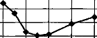
2
o
0 100 200 300 400 500 600
Fréquence (Hz)
Figure 43 : Résolution
fréquentielle (dF/F) en fonction de la fréquence de stimulation
pour 5 sujets
porteurs de l'implant cochléaire Digisonic.
La sensation de hauteur tonale sature en général entre 300 et 500 Hz (cf figure 44). Le codage temporel de la hauteur tonale (pitch rate) chez le sujet porteur d'un implant cochléaire dépend de l'étiologie. Lorsque le système auditif est bien conservé, il pourrait être supérieur à celui des normoentendants (Townshend et al, 1987). La stimulation électrique induirait une meilleure synchronisation (phase locking), ce qui corrobore les études sur la mesure de période réfractaire de neurones stimulés électriquement via un implant cochléaire (Abbas & Brown, 1991 ; Kasper, 1991).
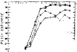

A
i?IgemriiÎescm(. 4 tos, the, tads)
liit
Es Es I.* ro
·
FREQUENCY <KHZ)
Figure 44 : Estimation de la tonie en fonction de la fréquence de stimulation, d'après Shannon, 1983
En résumé, pour les sujets porteurs d'implant cochléaire, le codage fréquentiel tonotopique est très réduit par rapport au sujet normo-entendant alors que le codage fréquentiel temporel est semblable voire meilleur selon l'étiologie de la surdité. Le codage de la parole chez le sujet porteur d'un implant cochléaire doit donc privilégier le codage de la fréquence de manière temporelle. Le codage fréquentiel temporel ne doit pas être négligé dans le traitement de stratégie de stimulation de l'implant cochléaire.
III Le codage en intensité
Le système auditif utilise plusieurs méthodes complémentaires pour coder les variations d'intensité de stimulation. Le codage se fait essentiellement par un accroissement du taux de décharge des fibres lorsque l'intensité de stimulation augmente. La dynamique des fibres est d'environ 30 à 40 dB ne suffit pas à expliquer la dynamique acoustique qui est de 100 à 120 dB. Liberman (1978), montre qu'il existe deux types de fibres de type I au niveau de la cochlée. Ils se différencient par leur diamètre et leur taux de décharge spontanée. D'un point de vue fonctionnel, les fibres ayant un petit diamètre et un taux de décharge spontanée supérieur à 18 potentiels d'action par seconde ont un seuil de déclenchement bas vers 0 dB HL. Les fibres ayant un gros diamètre et un taux de décharge spontanée inférieur à 18 potentiels d'action par seconde ont un seuil de déclenchement haut vers 40 à 50 dB HL. De 0 à 40-50 dB HL, le premier type de fibres (à seuils bas) code l'intensité de stimulation, les autres types de fibres sont inactifs. De 40-50 à 80-90 dB HL, les fibres à seuils hauts codent l'intensité de stimulation, les fibres à seuils bas sont saturées.
Le recrutement de fibres dû à un élargissement de la zone de cochlée stimulée lorsque l'intensité de stimulation s'accroît participe également au codage de l'intensité (Sacks et Abbas, 1974). Bien que les neurones codant la fréquence centrale de stimulation soient saturés, les neurones situés aux extrémités de la zone excitée peuvent coder l'intensité de stimulation.
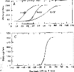
Figure 45 : Décharge des fibres auditives en
fonction de l'intensité acoustique (haut), électrique
(bas),
d'après Sachs et Abbas,1974 (Haut), Kiang et Moxon, 1972
(bas)
Pour le normo-entendant, le nombre d'échelons discriminés en intensité pour une fréquence donnée est d'environ 150, chez le sujet porteur d'un implant cochléaire il se situe entre 5 et 50 (Pfingst et al, 1983 ; Nelson et al, 1996). Le codage par type de fibres (seuils haut et bas) ne semble pas intervenir pour une stimulation électrique. De plus, la forte synchronisation produite par une stimulation électrique défavorise le codage par recrutement des fibres et augmente les pentes des courbes représentant les taux de décharge en fonction de l'intensité de stimulation. Le codage de l'intensité de stimulation par le nombre de potentiels d'action par seconde semble donc être le seul des trois systèmes de codage (taux de décharge, deux types de fibres, recrutement des fibres) utilisé par le sujet porteur d'un implant cochléaire. Ceci pourrait expliquer que le nombre de pas en intensité discriminé est plus faible que chez le normo-entendant et que la dynamique électrique varie de l'ordre de 2 à 20 dB alors que la dynamique acoustique est de 100 à 120 dB (Shannon, 1983 ; Pfingst et al, 1991) .
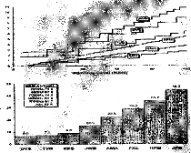
Figure 46 : Estimation du nombre de pas en
intensité pour différents patients implantés
cochléaires,
d'après Nelson et al, 1996
En résumé, la résolution en intensité chez le sujet porteur de l'implant cochléaire est beaucoup moins bonne que pour le normo-entendant et un seul des trois mécanismes (codage par taux de décharge) semble être utilisé pour coder l'intensité de stimulation.
L'objectif est de définir les caractéristiques du codage de l'intensité perçue par les sujets implantés cochléaires Digisonic (seuils de détection et de confort, seuils différentiels en intensité, sonie).
a- Seuils et dynamiques électriques
La plus petite et la plus grande quantité d'énergie perceptible par un système sensoriel sont d'abord déterminées par les propriétés biophysiques de l'organe sensoriel périphérique et des cellules transductrices. Les fonctions de seuils d'un système sensoriel reflètent en général les limitations physiques de l'organe périphérique à convertir l'énergie physique en impulsion nerveuse.
Avec un stimulus électrique, les propriétés biophysiques sont déterminées par l'activation du neurone par un champ électrique induit. Les seuils de détection et d'inconfort varient selon le patient. Il est nécessaire de détecter chacun d'eux sur toutes les électrodes lors de l'adaptation de l'interface bioélectrique. Les valeurs sont difficilement prévisibles. Il semble intéressant d'étudier les différents paramètres qui influencent la définition des seuils de détection et d'inconfort.
1- Seuils (détection et confort) et dynamiques en fonction du patient
Les spécificités de la stimulation électrique de l'implant cochléaire Digisonic, justifient l'étude des modifications de ses seuils de détection et de confort ainsi que celles des dynamiques en fonction du site stimulé et des caractéristiques du patient.
S. Gallégo, B. Frachet, E. Truy, L. Collet
Proceeding
du congrès SFA, 1998, sous presse
Cet article analyse avec un modèle par régression linéaire multiple les modifications des seuils (de détection et confort) et des dynamiques électriques en fonction des caractéristiques du patient. Trois paramètres ont été choisis, l'âge, la durée de privation et la durée d'implantation.
Pour quantifier ces modifications, nous avons utilisé une base de données comportant les seuils et dynamiques électriques de 80 sujets porteurs d'un implant cochléaire Digisonic sur une durée de 2 ans d'implantation sur les 15 électrodes.
Les résultats mettent en évidence des modifications très nettes des seuils en fonction de l'âge, de la durée de privation et de la durée d'implantation des patients.
La prise en compte de ces trois facteurs est donc importante lors des séances de réglage de l'implant cochléaire.
Modification des seuils en fonction des caractéristiques des sujets porteurs d'un implant cochléaire Digisonic
S. Gallégo (1,2), B. Frachet (3), E. Truy (2), L. Collet (2)
1- Laboratoires MXM, Vallauris
2- UPRESA- CNRS 5020, Lyon
3- Hôpital Avicenne, Bobigny e-mail: sgallegoemxmlab.com
La mise en place d'une technique objective (par Potentiels Evoqués Auditifs Electriques Précoces, ou Réflexe Stapédien) de mesure des seuils de détection (TL) (Gallégo et al, 1997) et de confort (CL) (Jerger et al, 1988) chez les implantés cochléaires est très importante. Elle permettrait d'obtenir un réglage chez les enfants et chez certains adultes lorsque le conditionnement apparaît difficile. Néanmoins ces techniques sont trop longues pour être utilisées en routine clinique pour toutes les électrodes. La possibilité d'obtenir les seuils (TL et CL) de toutes les électrodes à partir de seulement deux ou trois électrodes (Battmer et al, 1995) parait intéressante. D'après la littérature, plusieurs paramètres influencent les valeurs des seuils (TL et CL). Tout d'abord Lusted et al (1984), Shannon (1983), Pfingst et al (1980,1984) montrent que les seuils et la dynamique sont très dépendants de l'étiologie et de la population neurale du ganglion spiral des sujets implantés. Les seuils sont aussi très dépendants de la distance de l'électrode par rapport aux neurones à stimuler (Javel et al, 1987; Pfingst et al, 1980). L'orientation de la stimulation radiale ou longitudinale par rapport au porte électrode influence aussi les seuils (Pfingst et al, 1981). Le site de stimulation le long de la cochlée est aussi important car il existe des différences de quantité de neurones par millimètre carré en fonction de la tonotopie cochléaire et ganglionnaire (Hinojosa et al, 1985 ; Spoendlin et Schrott, 1988, 1989). Cette modification de la population neurale se traduit par des différences de la dynamique (Shannon, 1983).
Nous présentons les résultats d'une étude multicentrique Européenne réalisée sur une population de 80 sujets porteurs d'un implant cochléaire Digisonic. L'objectif de ce travail est d'étudier trois facteurs qui pourraient influencer les seuils et la dynamique des 15 électrodes (durée d'implantation, âge, durée de privation auditive).
L'implant cochléaire Digisonic
Le Digisonic est un implant cochléaire transcutané composé de 15 électrodes (Beliaeff et al, 1994). La partie implantée le long de la cochlée est composée d'un porte électrode sur lequel sont disposées 15 électrodes de 0.5 mm espacées de 0.7 mm. La zone stimulée se situe approximativement le long du premier tour de cochlée entre le cinquième et le vingtième millimètre par rapport à l'extrême base (Miller et al, 1993). Le mode de stimulation est appelé masse commune (une électrode stimule, toutes les autres sont à la masse). Sur le Digisonic le paramètre que l'on fait varier pour augmenter l'intensité de stimulation perçue (la sonie) est la durée de pulse (l'amplitude du pulse est constante). Cette durée est donnée en microseconde. Le courant injecté entre l'électrode de stimulation et les autre électrodes est de l'ordre de 1 mA (Gallégo et al, 1998). Quatre-vingt sujets porteurs de l'implant cochléaire multicanaux Digisonic ont participé à cette étude multicentrique Européenne (Bobigny Hôpital Avicenne (Fr) -
Paris Hôpital St Antoine (Fr) - North Riding
Infirmary, Middlesbrough (UK) - Istituto di Audiologie Milano (It) -
Marseille
Hôpital de la Timone (Fr) - Paris Hôpital Trousseau
(Fr) - CHU Grenoble (Fr) - CHU Bordeaux ( Fr) - Lyon Hôpital E.
Herriot
(Fr)). La population se compose de 41 femmes et 39 hommes. Les étiologies sont très variables. Une base de données contenant tous les réglages patients a été constituée avec en particulier les seuils (TL et CL) de chaque électrode (15 électrodes). Chaque fichier de réglages patient contient aussi la chronologie des différents réglages effectués depuis la première stimulation, jusqu'à 24 mois de suivi postopératoire. Pour participer à l'expérience et être retenues 12 sur 15 des électrodes des patients
devaient être fonctionnelles. On a choisi arbitrairement de numéroter les électrodes de la façon suivante : l'électrode 1 est la plus basale, l'électrode 15 la plus apicale.
Mesure de seuils de détection (TL) et de confort (CL) pour chaque électrode
Pour les réglages des seuils du sujet porteur de l'implant cochléaire Digisonic la mesure s'effectue à une fréquence de stimulation électrique fixe de 300 Hz. Pour éviter les phénomènes d'adaptation la stimulation est intermittente (0.5 seconde ON, 0.8 seconde OFF). Les seuils s'effectuent séparément sur les 15 électrodes en partant généralement de l'électrode la plus apicale (électrode 15) car celle-ci produit des sons plus facilement identifiables et très différents de sensations fantômes dues aux acouphènes (surtout lors des premiers réglages). Le seuil de détection (TL) correspond à un son à la limite de la perception, mais nettement audible. Le seuil de confort (CL) correspond à un son d'un niveau de sensation très fort mais supportable. Une fois les électrodes testées séparément, on procède à un équilibre des TL et CL par un balayage des électrodes basales aux électrodes apicales et un balayage des électrodes apicales aux électrodes basales pour ajuster les seuils. Cela permet d'équilibrer les niveaux de sonies aux TL et CL de toutes les électrodes. En plus des seuils, nous avons étudié la dynamique de chaque électrode. La dynamique se calcule en prenant dix fois le logarithme du rapport CL sur TL (dynamique = 10 Log (CL / TL)).
Seuils (TL et CL) et dynamiques moyens en fonction de l'électrode :
|
60 46 40 96 30 20 |
1 2 9 4 6 8 7 8 0 10 , 12 19 14 16
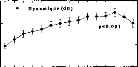
2 3 4 6 8 7 0 0 10 11 12 13 14 16
Numéro d'électrode (1:13m
15:
·pleale)
Figure 1: Valeurs moyennes et erreurs standards sur quatre-vingt sujets porteur d'un implant cochléaire Digisonic des seuils de détection (TL) confort (CL) (haut) ainsi que la dynamique (partie du bas) en fonction de l'électrode stimulée.
La figure 1 représente la moyenne et l'erreur standard sur 80 sujets porteurs d'un implant cochléaire Digisonic des TL et CL (partie du haut) et de la dynamique (partie du bas) en fonction de l'électrode stimulée. Les TL et CL sont indiqués en microseconde pour une stimulation de 1 mA. La dynamique est mesurée en dB électrique. Pour chaque sujet, on a pris la moyenne des différents seuils au cours du temps. Les TL et CL en fonction de l'électrode stimulée ont une forme appelée classiquement 'banane', ils sont semblables à ceux décrits par Battmer et al (1995) sur l'implant cochléaire Nucleus en stimulation 'common ground'. La dynamique est en moyenne de 2 à 4 dB électrique et est en accord avec les travaux de Shannon (1989).
L'étude statistique par une Anova ne trouve pas de dépendance entre le TL et la zone de cochlée stimulée (l'électrode stimulée). Les distances entre les neurones stimulés, l'électrode de stimulation, et l'état fonctionnel des neurones sont donc probablement peu dépendants de la zone de cochlée stimulée (numéro d'électrode). Par contre le CL et la dynamique sont dépendants de la zone de cochlée stimulée (p<0.001). D'après la littérature (Lusted et al, 1984 ; Shannon, 1983 ; Pfingst et al 1980, 1984), cela pourrait s'expliquer par des différences liées au nombre de neurones excités. De plus cela peut se confirmer par des corrélats anatomo-physiologiques (Hinojosa et al, 1985 ; Spoendlin et Schrott,1988, 1989) qui montrent chez le normo entendant un gradient croissant du nombre de cellules par millimètre carré jusqu'à la fin du premier tour de cochlée, puis une décroissance progressive jusqu'à l'apex. L'électrode 13 correspondrait à la zone où le nombre de neurones excités est le plus important car sa dynamique est maximale.
Etude des variations des seuils et dynamiques en fonction des différents paramètres
Une régression linéaire multiple entre les seuils et dynamiques pour chaque électrode et chacun des trois paramètres (durée d'implantation, durée de privation auditive avant implantation, âge du sujet) a été effectuée. Les résultats représentés correspondent aux coefficients qui relient les seuils et dynamiques à la variable étudiée (pentes des régressions linéaires). Pour chaque coefficient un test de significativité a été effectué (si p<0.05, le paramètre étudié fait varier significativement les seuils ou dynamiques).
Seuils (TL et CL) et dynamique en fonction de la durée d'implantation
TL CL DR
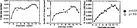
0 2 4 6 8 10 12 14
Electrode Number
0.2
0.01
j 0.00
à -0.01
-0.02
I
-0.03
.1
1 0.1
a
· 0.0
Y -0.04
C
e
-0.10
14 16
2 4 6 e 10 12 electrets number
2 4 6 e 10 12 14 16 Citerait number
· 0.008
0.007 v 0.006 e 0.005 e 0.004
· 0.003 t.r.e 0.002
· p<0.05
m p= NS
Figure 2 : Pentes sur 80 sujets porteurs d'un implant cochléaire Digisonic des seuils de confort (CL), des seuils de détection (TL), et de la dynamique en fonction de la durée d'implantation (en jours).
Les seuils de détection sont stables au cours du temps d'implantation (coefficient légèrement négatif). Par contre les seuils d'inconfort ainsi que les dynamiques, surtout dans la zone apicale, augmentent statistiquement en fonction du temps d'implantation (coefficient positif). De ces résultats plusieurs points positifs en ressortent. La constance, voire même la décroissance des seuils de détection, avec l'augmentation des seuils d'inconfort reflète une stabilité et une intégrité de l'interface bioélectrique. L'augmentation progressive de la dynamique pour chaque électrode montre une plasticité et une accoutumance du système auditif à la stimulation électrique.
Seuils (TL et CL) et dynamique en fonction de l'âge des sujets porteurs de l'implant
Les seuils de détection et de confort varient en fonction de l'âge des patients implantés. Ces modifications sont différentes en fonction du numéro d'électrode stimulé. Les seuils de détection et de confort augmentent en fonction de l'âge des sujets sur les électrodes apicales, inversement sur les électrodes basales. Ces résultats paraissent à priori surprenants mais il peuvent s'expliquer par un déplacement progressif du porte électrode en fonction de l'âge des sujets implantés par la croissance. Pour des raisons de difficulté d'insertion, le porte électrode se situe dans une zone plus basale de la cochlée lorsque le sujet est jeune. Ce déplacement pourrait aussi expliquer l'augmentation de la dynamique en fonction de l'âge des sujets (cf figure 1).
TL CL DR
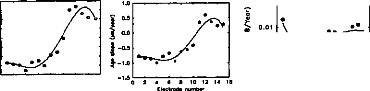

0.02

·
2 0.00
N
-0.01
t4
16
m 2 4 6 8 10 12 14
Electrode Number
2 4 6 6 10 12 Chocim«, number
0.2
0.1
I 0.0
-0.1
-0.2
I -0.3
I.
-0.4
-0.6
0.6
o
· p<0.05
m NS
Figure 3 : Pentes sur 80 sujets porteurs d'un implant cochléaire Digisonic des seuils de confort (CL), des seuils de détection (TL), et de la dynamique en fonction de l'âge des sujets implantés (en année).
Seuils (TL et CL) et dynamique en fonction de la durée de privation auditive
TL CL DR
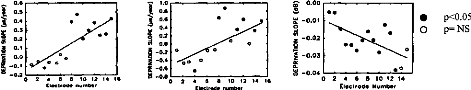
16
14
ît. 0.04
0
2 4 6 8 10 12 14
Elec1rode Numbor
2 4 6 8 10 12 Electro44 number
É -0.03
î
1.0
0.8
10.6
0.4
0.2
0.0
g -0.2
-0.4
t -0.6
0.00
· p<0.05 0 p= NS
Figure 4 : Pentes sur 80 sujets porteurs d'un implant cochléaire Digisonic des seuils de confort (CL), des seuils de détection (TL), et de la dynamique en fonction de la durée de privation auditive (en année).
Les seuils de détection, de confort et dynamique sont
très influencés par la durée de privation auditive.
Une
augmentation des seuils de détection et une diminution de la dynamique
peut s'expliquer par une
diminution de la population neurale et un moins bon fonctionnement du système auditif.
Conclusion
La prise en compte de l'évolution des seuils et de la dynamique des électrodes en fonction du temps
d'implantation, de l'âge du sujet, de la durée de
privation est donc nécessaire et intéressante pour
pouvoir
modéliser les seuils des 15 électrodes à partir de ceux
trouvés objectivement sur 1 à 3
électrodes. En effet
les techniques objectives ne permettent pas de détecter le TL et CL
simultanément.
Les potentiels évoqués auditifs électriques précoces (PEAEPs) peuvent nous donner le TL (Gallégo et al, 1997); le réflexe stapédien nous donne uniquement le CL (Jerger et al, 1988).
Références
Battmer R-D, Gnadeberg D, Allum-Mecklenburg DJ. Algorithmic representation of common ground Programming in children with the Nucleus Device. Adv Otorhinolaryngol, Basel, Karger, 1995 50 83-90
Beliaeff M, Dubus P, Leveau JM, Repetto JC, Vincent P. Sound processing and stimulation coding of Digisonic DX10 15- channel cochlear implant. Hochmair IN, ed. Advances in cochlear implant. Innsbruck: Verlag. 1994 198-203
Gallégo S, Truy E, Morgon A, Collet L. EABRs and surface potentiels with a transcutaneous multielectrode cochlear implant. Acta Otolaryngol (Stockh) 1997 117:164-168
Gallégo S, Luu BL, Berger-Vachon C. Modelling of electrical stimulation delivered by the Digisonic Multichannel cochlear implant. Advance Modelling Signal Eng, 39,1, 39-53
Hinojosa R, Seligsohn R, Lerner S. Ganglion cell counts in the cochleae of patients with normal audiograms. Acta Otolaryngol (Stockh) 1985 99:8-13
Javel E, Tong Y, Shepherd B, Clark G. Responses of cat auditory nerve fibers to biphasic electrical current pulses. Ann Otol Rhinol Laryngol 1987 96(sup 128):26-30
Jerger J, Olivier TA, Chmiel RA. Prediction of dynamic range from stapedius reflex in cochlear implanted patients. Ear Hear 1988 9:4-8
Lusted H, Shelton C, Simmons S. Comparison of electrode sites in electrical stimulation of the cochlea. Laryngoscope 1984 94:878-882
Miller CA, Abbas PJ, Brown CJ. Electrically evoked auditory brainstem response to stimulation of different sites in the cochlea. Hear Res 1993 66:130-42
Pfingst B, Telman S, Sutton D. Operating ranges for cochlear implants. Mn Otol Rhinol Laryngol 1980 89(sup 66):1-4 Pfingst B, Sutton D, Miller J, Bohn B. Relation of psychophysical data to hystopathology in Monkeys with cochlear implant. Acta Otolaryngol (Stockh) 1981 92:1-13
Pfingst B. Operating ranges and intensity psychophysics for cochlear implants. Arch Otolaryngol 1984 110:140-144
Shannon RV. Multichannel electrical stimulation of the auditory nerve in man.l. Basic psychophysics. Hear Res 1983 11:157- 89
Shannon RV. A model of threshold for pulsatile electrical stimulation of cochlear implants. Hear Res 1989 40:197-204 Spoendlin H, Schrott A. The Spiral Ganglion and the Innervation of the Human Organ of Corti. Acta Otolaryngol (Stockh) 1988 105:403-10
Spoendlin H, Schrott A. Analysis of the human auditory nerve. Hear Res 1989 43:25-38
L'article précédant ayant montré une nette modification des seuils et dynamiques électriques en fonction de la durée d'implantation, il paraît intéressant d'étudier plus précisément la part liée à la modification de l'interface bio-électrique et celle liée à plasticité neurale sur l'évolution de ces seuils
S. Gallégo, B. Frachet, C. Berger-Vachon , L.
Collet
Article soumis
Cet article décrit et interprète les modifications des seuils et les dynamiques électriques en fonction de la durée d'implantation.
La stabilité du seuil de détection après les 100 jours d'implantation ainsi qu'une augmentation progressive de la dynamique électrique démontre une stabilité de l'interface bio-électrique et une préservation de la population neurale du système auditif.
L'évolution de la dynamique électrique et du seuil d'inconfort montre une adaptation progressive du système auditif à la stimulation électrique. Afin de prendre en compte les modifications de l'interface bio-électrique et des capacités du sujet implanté cochléaire, il est nécessaire d'effectuer des réglages réguliers du processeur vocal.
LONG-TERM CHANGE IN THRESHOLD AND COMFORT LEVELS
AND
DYNAMICS IN DIGISONIC COCHLEAR IMPLANT BEARERS
S. Gallégo", B. Frachet3,C. Berger-Vachonl, L.
1- UPRESA- CNRS 5020 laboratory
2- MXM laboratory
3- ORL department, Avicenne Hospital
ABSTRACT : Variations in threshold level (TL), comfort level (CL) and dynamics were studied in a population of 80 subjects fitted with the Digisonic cochlear implant, a French multichannel implant manufactured by the MXM company. Statistical analysis, by Anova, showed very significant changes in CL and dynamics over implantation time. This may be explained by neuronal plasticity facilitating auditory system adaptation to the electrical stimulation. Results for TL over implantation time further showed the implant system to be stable and not destructive of the auditory nervous system. This may be due to the fact that each electrode of the Digisonic implant has an in-series capacity which very accurately controls and balances the number of positive and negative charges. Such a charge balance is vital to avoid electrolysis between electrode and physiological environment.
Key words: Cochlear Implantation, Threshold, Dynamic range, Auditory plasticity, Integrity system
INTRODUCTION
It is very important to develop an objective means, using Electrical Auditory Brainstem Responses or Stapedius Reflex, of measuring threshold level (TL) (Gallégo et al, 1997) and comfort level (CL) (Jerger et al, 1988) in cochlear implant bearers, to enable setting in children and in certain adults when conditioning is a problem. These techniques, however take too long for routine clinical application on all the electrodes. It would thus be very interesting to be able to determine TL and CL for the whole set of electrodes on the basis of just two or three of them (Battmer et al, 1995).
According to the literature, there are several parameters affecting TL and CL values. Firstly, Lusted et al (1984), Shannon (1983), Pfingst et al (1980, 1984) have shown levels and dynamics to be ciosely dependent on subjects' aetiology and spiral ganglion neurone population. The levels also very much depend on the electrode's distance from the neurones to be stimulated (Javel et al, 1987 ; Pfingst et al, 1980). Whether stimulation is radial or longitudinal in relation to the electrode holder also affects levels (Pfingst et al, 1981). The position of the stimulation site along the cochlea is also important as there are differences in neurone density according to cochlear and ganglion tonotopy (Hinojosa et al, 1985 ; Spoendlin et Schrott, 1988, 1989), and this is reflected in differences in dynamics (Shannon, 1983).
Here are presented the results from a European multi-centric study involving 80 Digisonic Implant bearers which sought to determine implant duration effects on the levels and dynamics of the 15 electrodes.
MATERIAL & METHODS
The Digisonic cochlear implant
The Digisonic is an transcutaneous cochlear implant comprising 15 electrodes (Beliaeff et al, 1994). Digital signal processing is by Fast Fourier Transform (FFT), with real-time calculation of acoustic signal spectrum over 64 frequency bands between 122 and 7800 Hz. Each electrode corresponds to a set of frequency bands. The part of the apparatus implanted along the cochlea consists of an electrode holder carrying 15 0.5 mm electrodes at 0.7 mm intervals. The stimulated area runs round the first arm of the cochlea roughly from the fifth to the twentieth millimetre from the basal extremity (Miller et al, 1993) -- i.e., roughly speaking, the area coding for 1-16 kHz frequencies. Stimulation is in what is called the common ground mode : for one electrode stimulated all the others act as ground. In the Digisonic, the parameter which varies to increase the intensity of the sound, or perceived stimulus, is the pulse-time, in microseconds, pulse amplitude being constant. The current injected between the stimulation electrode and the others is of the order of 1 mA (Gallégo et al, submitted).
Cochlear implant subjects
80 multichannel Digisonic cochlear implant bearers took part in this multicenter European study (*): 41 female, 39 male. 43 had right implants, 30 left, and data were missing for 7. Aetiologies were very varied. Mean hearing deprivation duration was 11.9 years (s.d. = 14.5 years) for a range from 0.3 year to 62 years.
A database of ail patient settings was created on Excel, containing in particular TL and CL values for each of the 15 electrodes. Each patient's setting file also contained the history of setting from first stimulation to 24 moths' post-operative follow-up. An inclusion criterion was that 12 of the 15 electrodes were should be working. The electrodes were arbitrarily numbered 1 to 15, basal to apical.
(*) Bobigny Hôpital Avicenne (Fr) - Paris Hôpital St Antoine (Fr) - North Riding lnfirmary, Middlesbrough (UK) - Istituto di Audiologia Milano (It) - Marseille Hôpital de la Timone (Fr) - Paris Hôpital Trousseau (Fr) - CHU Grenoble (Fr) - CHU Bordeaux ( Fr) - Lyon Hôpital E. Herriot (Fr)
Threshold (TL) and comfort (CL) level measurement for the 15 electrodes
Level setting measurement for Digisonic cochlear implant bearers is performed at a fixed electrical stimulation frequency of 300 Hz. To avoid adaptation effects, the stimulation is intermittent : 0.5 sec. ON, 0.8 sec. OFF.
The 15 electrodes are set individually, usually starting from the most apical (n° 15) as this one produces the most easily identifiable sound, quite different from phantom sensations due to tinnitus (particularly at first setting).
TL corresponds to a sound at the limit of perceptibility while still clearly audible. CL corresponds to a sound of very high sensation level but which is still bearable. After testing the electrodes individually, TL and CL are balanced by sweeping basal-toapical and apical-to-basal to adjust levels (TL and CL). Thus sound levels can be balanced against the TL and CL of all electrodes.
As well as these levels, the dynamics of each electrode was studied, calculated as ten times the Iogarithm of CL over TL (dynamics = 10 LOG ( CL / TL) ).
RESULTS & DISCUSSION
Mean TL, CL and dynamics per electrode
|
50 45 40 35 30 25 20 15 |
1 2 3 4 5 6 7 8 9 10 11 12 13 14 15
|
4 3 2 1 |
||
|
1 2 3 4 5 6 7 8 9 10 11 12 13 14 15 Electrode Num ber (1:basal 15:apical) |
||
Figure 1 : Mean values and standard errors for threshold level (TL) and comfort level (CL) (above) and dynamics (below) per electrode in 80 Digisonic cochlear implant bearers.
Figure 1 shows means and standard errors for TL and CL (above) and dynamics (below) per electrode in 80 Digisonic cochlear implant bearers. TL and CL are in microseconds of 1 mA stimulation, and dynamics is in electrical dB. For each subject, mean levels over time are shown. TLs and CLs per electrode show what is classically known as a "banana" form, similar to that described by Battmer et al (1995) for the Nucleus cochlear implant in "common ground" stimulation mode. Dynamics averaged 2 to 4 electrical dB, in agreement with Shannon's findings (1989) of narrow dynamics for pulse-times less than 100 ps without this affecting the number of sound levels.
Repeated measure Anova analysis found no correlation between TL and cochlear area (i.e. electrode number) stimulated. The distance between the stimulated
neurones and the stimulating electrode, and also the functional condition of the neurones, are therefore probably fairly independent of the cochlear area stimulated (i.e. electrode number).
CL and dynamics, on the other hand, did depend on cochlear area (p<0.001). On the basis of the literature (Lusted et al, 1984 ; Shannon, 1983 ; Pfingst et al, 1980, 1984), this could be explained in terms of differences relating to the number of neurones stimulated. This is borne out by anatomo-physiological correlates which, in normalhearing subjects, show a rising gradient of cell density up to the end of the first arm of the cochlea followed by a graduai decrease to the apex (Hinojosa et al, 1985 ; Spoendlin et Schrott, 1988, 1989). Electrode 13 should correspond to the area of maximum number of stimulated neurones, its dynamics being the highest.
TL, CL and dynamics over implantation time
Figure 2 shows means and standard errors for CL (above), TL (middle) and dynamics (below) per electrode in 80 Digisonic cochlear implant bearers at different periods of implantation. And figure 3, similarly, shows means and standard errors for CL (above), TL (middle) and dynamics (below) for the average of the 15 electrodes in the same population. CL and TL are in microseconds of 1 mA stimulation, and dynamics is in electrical dB. Two-way repeated measure Anova (for electrode stimulated and implantation time) revealed the following findings.
Changes in TL, CL and dynamics with implantation time depended on stimulated number (p=0.008 for TL, p<0.001 for CL and p<0.001 for dynamics) (figure 2).
TL fell until day 100, suddenly rose, then plateaued (p<0.001). The fall until day 100 may be explained by enhanced threshold detection on the part of the implanted subject, by neuronal plasticity and by post-operative cicatrisation.
The sudden change in TL after 100 days has been previously described in the literature (Clark et al, 1988). A study in guinea-pigs showed, psycho-physically and electrophysiologically (Miller et ail, 1995), a sudden change in TL between days 50 and 140 of implantation. This corresponds to two phenomena: firstly, progressive degeneration of spiral ganglion dendrites projecting onto the cochlea, entailing an increased electrode-to neurone distance ; and, secondly, slight fibrosis along the
electrode holder, altering environmental impedance. That TL plateaux afterwards
70 60 50 40 30
20 26 24 22 20 18 16 14 12 6
5 4 3 2
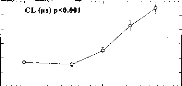
10 100 1000
TL (rts) p<0.001
10 100 1000
Dynamic (dB) p<0.001'
10 100 1000
Days after implantation
55 50 45 40 35 30 25
22 20 18 16 14 5 4 3 2
shows that the interface between physiological environment and electrode stabilises, which is due to the Digisonic implant's perfect control of charge through the electrodes by coupling capacity. Continued rise in TL over implantation time would have indicated progressive auditory system degeneration due to electrolysis because of poor charge control.
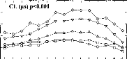
1 2 3 4 5 6 7 8 9 10 11 12 13 14 15
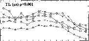
1 2 3 4 5 6 7 8 9 10 11 12 13 14 15
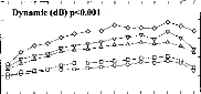
1 2 3 4 5 6 7 8 9 10 11 12 13 14 15
Electrode number (1:basal 15:apical)
o <20 days y 140< <300 days
· 20< <60 days 300< <640 days
· 60«140 days
Figure 2 : Mean values and standard errors for Comfort level (CL) (above), threshold level (middle) and dynamics (below) per electrode at various post-implantation periods (0-20, 20-60, 60-140, 140-300 and 300-640 days) in 80 Digisonic cochlear implant bearers.
Figure 3 : Mean values and standard errors for Comfort level (CL) (above), threshold level (middle) and dynamics (below) for the whole electrode set at various post-implantation periods (0-20, 20-60, 60-140, 140-300 and 300-640 days) in 80 Digisonic cochlear implant bearers.
Unlike TL, CL and dynamics increased progressively over implantation time (Kubo et al, 1996). In two years, each electrode's dynamics doubied. These findings agree with those of Miller et al (1995) in guinea pigs. This increase in CL and in dynamics is a matter of neuronal plasticity, the auditory system becoming ever better at encoding
intensity. This plasticity is probably due to the auditory nervous system's having to adapt to much higher neuronal discharge rates (in spike/sec.) with electrical as compared to acoustic stimulation (Kiang and Moxon, 1972) and the much greater fiber synchronisation greatly strengthens neuronal interaction under electrical stimulation, considerably lowering CL and thus reducing dynamics.
The questions raised by the change over time in individual electrode dynamics are: how does the auditory system adapt to cope with the electrical stimulation, and what are the consequences for cochlear implant bearers' performance development over time (Spivak et Walzman, 1990 ; Kubo et al, 1996) ?
CONCLUSION
A study of TL and CL in a population of 80 Digisonic cochlear implant bearers over a period of two years revealed very significant change with implantation time. Intensity encoding capability increases (neuronal plasticity). The study further showed that Digisonic cochlear implant causes no progressive auditory system degeneration.
It is therefore both necessary and interesting to take change over implantation time in electrode levels and dynamics into account to model levels for all 15 electrodes on the basis of objective measurements in 2 or 3. Objective techniques do not allow simultaneous determination of TL and CL: EABRs can give TL (Gallégo et al, 1997), and Stapedius Reflex gives only CL (Jerger et al, 1988).
REFERENCES
Battmer R.D., Gnadeberg D., AIIum-Mecklenburg D.J. (1995) Algorithmic representation of common ground Programming in children with the Nucleus Device. Adv Otorhinolaryngol, Basel, Karger, 50 83-90.
Beliaeff M., Dubus P., Leveau J.M., Repetto J.C., Vincent P. (1994) Sound processing and stimulation coding of Digisonic DX10 15-channel cochlear implant. Hochmair IN, ed. Advances in cochlear implant. Innsbruck: Verlag. pp. 198-203.
Clark G., Shepherd R., Franz B., Dowell R., Tong Y. (1988) The histopathology of the human temporal bone and auditory central nervous system following cochlear implantation in patient. Acta Otolaryngol. (Stockh) (suppl 448), 1-65.
Gallégo S., Truy E., Morgon A., Collet L. (1997) EABRs and surface potentials with a transcutaneous multielectrode cochlear implant. Acta Otolaryngol. (Stockh) 117, 164-168.
Gallégo S., Luu B.L., Berger-Vachon C. (in press) Modelling of electrical stimulation delivered
by the Digisonic Multichannel cochlear implant. Advance Modelling Signal Eng.
Hinojosa R., Seligsohn R., Lerner S. (1985) Ganglion cell counts in the cochleae of patients
with normal audiograms. Acta Otolaryngol. (Stockh) 99, 8-13.
Javel E., Tong Y., Shepherd B., Clark G. (1987) Responses of cat auditory nerve fibers to
biphasic electrical current pulses. Ann. Otol. Rhinol. Laryngol. 96(sup 128), 26-30.
Jerger J., Olivier T.A., Chmiel R.A. (1988) Prediction of dynamic range from stapedius reflex in
cochlear implanted patients. Ear Hear. 9, 4-8.
Kiang N.Y.S., Moxon E.C. (1972) Physiological considerations in artificial stimulation of inner ear. Ann. Otol. 81, 714-730.
Kubo T., Iwaki T., Ohkusa M., Dol K., Uno A., Yamamoto K., Fujii K. (1996) Auditory plasticity in cochlear implant patients. Acta Otolaryngol. (Stockh) 116, 224-227.
Lusted H., Shelton C., Simmons S. (1984) Comparison of electrode sites in electrical stimulation of the cochlea. Laryngoscope 94, 878-882.
Miller C.A., Abbas P.J., Brown C.J. (1993) Electrically evoked auditory brainstem response to stimulation of different sites in the cochlea. Hear. Res. 66, 130-142.
Miller C.A., Faulkner M.J., Pfingst B.E. (1995) Functional responses from guinea pigs with cochlear implants II. Changes in electrophysiological and psychophysical measures over time. Hear. Res. 92, 100-111.
Pfingst B., Telman S., Sutton D. (1980) Operating ranges for cochlear implants. Ann. Otol. Rhinol. Laryngol. 89(sup 66), 1-4.
Pfingst B., Sutton D., Miller J., Bohn B. (1981) Relation of psychophysical data to hystopathology in Mon keys with cochlear implant. Acta Otolaryngol. (Stockh) 92, 1-13.
Pfingst B. (1984) Operating ranges and intensity psychophysics for cochlear implants. Arch. Otolaryngol. 110, 140-144.
Shannon RV. (1983) Multichannel electrical stimulation of the auditory nerve in man.l. Basic psychophysics. Hear. Res. 11, 157-189.
Shannon RV. (1989) A model of threshold for pulsatile electrical stimulation of cochlear implants. Hear. Res. 40, 197-204.
Spivak L.G., Waltzman S.B. (1990) Performance of cochlear implant patients as a function of time. J. Speech. Hear. Res. 33, 511-519.
Spoendlin H., Schrott A. (1988)The Spiral Ganglion and the Innervation of the Human Organ of Corti. Acta. Otolaryngol. (Stockh) 105, 403-10.
Spoendlin H., Schrott A. (1989) Analysis of the human auditory nerve. Hear. Res. 43, 25-38.
2-Seuils en fonction de la fréquence de stimulation
D'après la littérature, les seuils de détection et les dynamiques électriques décroissent progressivement en fonction de la fréquence de stimulation (Shannon 1983, Pfingst et al, 1991, 1993). La fonction qui fait correspondre les seuils de détection à la fréquence de stimulation est très variable, selon le sujet ; il n'existe pas de corrélation franche entre les seuils de détection pour deux fréquences de stimulation (Brown et al, 1999).
50
500
1000
-35 10
Figure 47 Modification des seuils en fonction de la fréquence de stimulation, d'après Pfingst, 1991
Toutes ces études ont utilisé l'amplitude de l'impulsion pour coder l'intensité de stimulation. De plus la forme de l'impulsion était symétrique. L'étude des modifications des seuils et dynamiques électriques en fonction de la fréquence de stimulation via la stimulation de l'implant cochléaire Digisonic semble donc importante pour la mise en place de stratégie de codage à des fréquences de stimulation variables.
Nous avons mesuré les seuils de détection (TL) et de confort (CL) sur trois électrodes (électrode basale :1 à 5, électrode médium : 6 à10, électrode apicale :11 à 15) à 4 fréquences de stimulations différentes (75, 150, 300, et 600 Hz) chez une population de 16 implantés cochléaires Digisonic. Pour éviter les phénomènes d'adaptation, la stimulation est intermittente (0.43 seconde ON et 1 seconde OFF). Le paramètre utilisé pour faire varier l'intensité de stimulation est la durée de l'impulsion (en ps). Le courant injecté entre l'électrode de stimulation et les autres est de 1 mA. Afin d'atténuer la fatigue auditive, nous avons d'abord mesuré les TL, puis les CL.
Le seuil de détection (TL) correspond au seuil absolu de perception. Pour pouvoir le mesurer très
précisément nous avons commencé par stimuler à un niveau de sonie nettement perceptible pour que
le sujet puisse repérer le son, puis nous avons diminué l'intensité de stimulation jusqu'à la disparitiontotale de la sensation. Le TL correspond au dernier niveau d'intensité auquel le sujet a entendu un son. Cette technique permet au sujet de suivre le son jusqu'à des intensités de stimulation très faibles.
Le seuil d'inconfort (CL) correspond à un niveau d'intensité juste au-dessous de la douleur. Tout comme la mesure du TL, il faut commencer par stimuler à un niveau de sonie moyen, puis augmenter progressivement l'intensité de stimulation jusqu'à atteindre un niveau de sensation proche de la gêne. Cette technique permet de limiter la fatigue auditive et de protéger le sujet de sons qui pourraient être désagréables.
En plus des seuils, nous avons étudié la dynamique de chaque électrode. La dynamique se mesure en décibel (dynamique =10 Log (CL/TL)).
La partie haute de la figure 48, représente la moyenne pour la population des 16 implantés cochléaires des seuils de détection et de confort pour trois zones de cochlée différentes en fonction de la fréquence de stimulation. Les valeurs sont indiquées en décibel, ce qui correspond à 10 log de la durée de l'impulsion en ps.
La partie basse de la figure 48, représente la moyenne pour la population des 16 implantés cochléaires des dynamiques électriques pour trois zones de cochlée différentes en fonction de la fréquence de stimulation.
L'analyse statistique par une Anova à deux facteurs (la fréquence de stimulation et la zone de cochlée stimulée) sur mesures répétées (les patients)
- ne montre pas de modification du TL en fonction de la zone stimulée (p>0.1) et en fonction de la fréquence de stimulation (p=0.079)
- indique une variation statistique du CL en fonction
- de la zone stimulée (p<0.001). La région apicale est différente des régions basale et médium. - de la fréquence de stimulation (p<0.001). Les fréquences 300 et 600 Hz ne sont pas différentes statistiquement.
- indique une variation statistique de la dynamique électrique en fonction
- de la zone stimulée (p<0.001). La région apicale est différente des régions basale et médium. - et de la fréquence de stimulation (p<0.001). Les fréquences 300 et 600 Hz ne sont pas différentes statistiquement.
5
75 Hz
150 Hz 300 Hz 600 Hz
75 Hz 150 Hz 300 Hz 600 Hz
·Apicale
10
9
H
7! . 8 z
1 7
k
6
75 Hz 150 Hz 300 Hz 600 Hz
Médium
10
150 Hz 300 Hz 600 Hz
9
e
8
Ef
5 7
6
5
75 Hz
75 Hz 150 Hz 300 Hz 600 Hz
75 Hz 150 Hz 300 Hz 600 Hz
Basale
23
23
21ie 19
0.17e 15
21
11
g 13
11
9
9
10
9
3 8
5 76
5
23
21
19
3 . I 7
2 15 ZI 13
11
9
1 I
· 1TL (dB) -18- CL (dB)
II (dB) -81.. CL (dB)
Figure 48 : Moyenne des seuils de détection et de confort en dB ps et dynamique électrique en dB
chez une population de 16 sujets implantés cochléaires Digisonic en fonction de la fréquence de
stimulation pour différentes zones stimuléesLe fait que les seuils de détections soient très peu sensibles à la fréquence de stimulation est contradictoire avec les résultats obtenus avec d'autres systèmes implantés (Shannon, 1983, Pfingst, 1991). Cela peut sûrement s'expliquer par les caractéristiques du stimulus électrique qui sont très différentes de celles des autres systèmes. En effet, avec l'implant cochléaire Digisonic la durée et non l'amplitude de l'impulsion sert à coder la sonie ; cette durée est très faible au seuil de détection (de 5 à 20 ps généralement), ce qui augmente la synchronisation des fibres. De plus l'impulsion qui est asymétrique stimule le nerf principalement sur sa phase positive. Tout cela fait que le seuil de détection est très stable d'une mesure à une autre et est très peu dépendant de la fréquence de stimulation.
Le fait que le seuil de détection varie peu en fonction du site de stimulation provient principalement du mode de stimulation en masse commune et du fait que la distance et l'impédance entre les électrodes de stimulations et les neurones du ganglion spiral à stimuler sont peu dépendants de la zone stimulée.
Les modifications des seuils d'inconfort et des dynamiques en fonction de la fréquence de stimulation s'expliquent par l'augmentation de la sonie en fonction du nombre de charge injectée par seconde. Les CL et la dynamique sont dépendants de la zone de cochlée stimulée. D'après la littérature (Lusted et al, 1984 ; Shannon, 1983 ; Pfingst et al 1980, 1984), cela pourrait s'expliquer par des différences liées au
nombre de neurones excités. De plus cela peut se confirmer par des corrélats anatomo-physiologiques
(Hinojosa et al, 1985 ; Spoendlin et Schrott,1988, 1989) qui montrent chez le sujet normo-entendant un gradient croissant du nombre de cellules par millimètre carré jusqu'à la fin du premier tour de cochlée, puis une décroissance progressive jusqu'à l'apex.
3- Seuils en fonction de la durée de stimulation
Il est important de savoir si, tout comme lors d'une stimulation acoustique, une stimulation électrique prolongée de la cochlée engendre une diminution progressive de la sonie. Ce phénomène appelé adaptation de sonie est notamment très important lors d'atteinte retro-cochléaire.
Proceeding du Congrès de la Société Française d'Audiologie, Clermont-Ferrand, décembre 1998
Cet article mesure les variations du seuil de détection en fonction du temps de stimulation par le 'tone decay test'.
Ce phénomène d'adaptation de sonie est fonction de la zone cochléaire activée lors d'une stimulation acoustique (Hellman et al, 1997), mais aussi de la cadence de stimulation lors d'une stimulation par clic acoustique.
L'étude sur 12 sujets implantés cochléaires Digisonic ne montre pas de variation de l'adaptation de sonie selon la zone cochléaire stimulée. Par contre, la cadence de stimulation influence positivement l'adaptation de sonie.
Cette adaptation de sonie est comparable à celle observée chez le normo-entendant et est en moyenne de 10 à 30 % de la dynamique électrique (Miskiewicz et al, 1993).
ADAPTATION CHEZ LES SUJETS PORTEURS D'UN IMPLANT COCHLEAIRE DIGISONIC.
Wable J., Gallégo S.*, Roussillon I., et Frachet B.
CRISTAL, Hôpital Avicenne, Service ORL, 125 rue de Stalingrad, 93009 Bobigny, France. * MXM 2720 Chemin St Bernard F-06224 Vallauris Cedex, France.
Introduction
La diminution de la sonie d'un son au cours d'une stimulation continue est un phénomène appelé adaptation de sonie ou 'tone-decay'. Cette fatigue auditive est liée à la diminution de la réponse du récepteur et à une habituation du système auditif central, a été étudié essentiellement étudiée à l'aide de stimulations acoustiques. L'évaluation de l'adaptation de sonie chez des sujets implantés pourrait apporter des informations sur l'état du système auditif de ces patients : excitabilité des neurones, capacités de récupération. Le fait que les stimulations soient électriques et non acoustiques influence les propriétés d'excitation des neurones et peut donc modifier le phénomène d'adaptation. D'autre part, la variabilité de l'adaptation entre les sujets pourrait et expliquer une partie de la variabilité des performances. La présence d'adaptation chez les implanté cochléaires est controversée (Shannon, 1983 ; Brimacombe & Eisenberg, 1984). Ces derniers auteurs ne l'observent que chez 3 de leur 17 sujets. Shannon (1983) l'observe de manière plus fréquente. Cependant il suggère que l'altération du système auditif chez les sourds profonds est peut-être à l'origine d'une dégradation du processus d'adaptation chez les porteurs d'implant cochléaire et que par conséquent l'adaptation observée lors d'une stimulation électrique ne soit pas de même nature que celle observée lors d'une stimulation acoustique.
Notre étude a pour objectif d'évaluer l'adaptation de sonie chez les sujets implantés porteur d'un implant Digisonic. Ces données d'adaptation seront confrontées avec les performances à des tests phonétiques. L'objectif final est de pouvoir mieux régler les paramètres de l'implant (seuils, cadence de stimulation, nombre d'électrodes actives...), de proposer un test permettant d'évaluer le fonctionnement du système auditif des patients.
Matériel et méthodes Sujets
12 sujets porteurs de l'implant Digisonic DX10 ont été inclus dans l'étude. Seuls les données de 7 d'entre eux, complètes, sont analysées ici. La durée de privation auditive pour ce groupe est comprise entre 1 et 7 ans, la durée d'implantation entre 7 et 42 mois, l'âge entre 42 et 71 ans.
L'implant Digisonic
L'implant Digisonic est décrit plus en détail dans l'article ' Existe-t-il une relation entre les potentiels évoqués de latence tardive et la reconnaissance de la parole chez les implantés cochléaires ? ' de ce même recueil, de même que par Beliaeff et al. (1984). Avec le type de stimulation utilisé pour cet implant le niveau d'intensité se mesure en ;as.
Test d'adaptation
Le test de mesure de l'adaptation, ou tone decay en anglais, consiste à évaluer, sur une période de temps déterminé, le niveau d'intensité dont il faut augmenter un son continu présenté initialement au seuil de perception pour que la sensation persiste pendant une durée déterminée.
En pratique, le niveau seuil est déterminé ; puis, le stimulus continu est présenté à ce niveau et chaque fois que le patient indique que le son n'est plus perceptible, l'expérimentateur augmente le niveau. Le pas d'incrémentation est de 1 its. La quantité d'adaptation correspond au nombre d'incréments nécessaires pour que la perception soit maintenue pendant 1 minute. Le niveau maximum confortable est ensuite évalué avec une stimulation discontinue.
Deux facteurs ont été considérés :
· la position des électrodes testées : 3, 6, 9, 12, et 15 en général ; une électrode proche lorsque l'une de celles-ci est inactivée chez un patient.
· la cadence de stimulation : 170 Hz et 310 Hz,
Trois mesures répétées ont été effectuées pour chacune des conditions.
D'éventuelles corrélations entre la quantité d'adaptation et les performances de reconnaissance de la parole ont été recherchées.
La quantité d'adaptation a été mesurée initialement en las puis rapportée à un pourcentage en fonction de la dynamique.
Tests phonétiques
Les tests consistent à évaluer la reconnaissance de sons, mots ou phrases sans l'aide de la lecture labiale. Les différents tests réalisés sont les suivants :
· reconnaissance de logatomes VCV : 16 consonnes sont testées, chacune est présentées trois fois,
· reconnaissance de mots monosyllabiques (listes de Lafon) : 1 liste est présentée, ce qui correspond à 17 mots, 51 phonèmes,
· reconnaissance de mots monosyllabiques : 75 mots, reconnaissance de phrases : 35 phrases contenant 119 mots clés,
· répétition d'un texte : le sujet répète le texte lu par l'expérimentateur. Celui-ci répète le texte jusqu'à ce que le sujet ait tout compris. Le nombre de mots reconnus en 5 minutes est évalué.
Les stimuli sont présentés soit par l'expérimentateur soit par un ordinateur. Le processeur de l'implant est réglé par le sujet à un niveau confortable. Le sujet répète ce qu'il a entendu même si cela lui paraît aberrant ou dépourvu de sens.
Analyse
Lorsque le nombre de sujet le permettra, l'adaptation de sonie sera analysée selon plusieurs paramètres :
(1) paramètres de réglage : le niveau seuil, le niveau maximum confortable, la dynamique, la cadence de stimulation, la position des électrodes.
(2) paramètres cliniques : durée de la surdité, âge, durée de l'implantation
(3) paramètres psychométriques : performances aux tests phonétiques.
Actuellement, seuls les effets des facteurs cadence de stimulation et position des électrodes ont été évalués par une analyse de variance sur mesures répétées.
Résultats
Test d'adaptation
Un seul sujet ne présente aucune adaptation quelle que soit la condition. Lorsque l'adaptation est présente, sa valeur varie de 1 à 6 lis. Lorsque la quantité d'adaptation est rapportée à la dynamique (en %), l'analyse statistique (ANOVA à deux facteurs) met en évidence un effet de la cadence seulement (F = 20.8 ; p = 0.04) (Figure 2). La quantité d'adaptation est plus élevée, pour la cadence de stimulation la plus élevée (Figure 1).
·310 Hz
|
60% 50% 40% 30% 20% 10% 0% |
|||
1 2 3 4 5 6 7 8 9 10 11 12 13 14 15
Electrode
Figure 1- Adaptation (en % de la dynamique) en fonction de la cadence et de la position des électrodes
Corrélation avec les tests phonétiques
Les performances aux test phonétiques sont les suivantes (N=7) :
|
Test % |
VCV |
Mots |
Phrases |
Lafon IC+LL |
Lafon IC seul |
|
Etendue |
27-67 |
11-57 |
21-90 |
77-96 |
45-82 |
|
Moyenne |
48 |
40 |
60 |
89 |
65 |
L'étude statistique n'a pas mis en évidence de corrélation entre la quantité d'adaptation exprimée en pourcentage et les performances aux tests phonétiques. Toutefois, le faible nombre actuel de sujets ne donne pas une puissance satisfaisante au test.
Perspectives
Une augmentation du nombre de sujets dans cette étude permettra d'établir des valeurs normatives de l'adaptation de sonie chez les patients porteurs d'un implant Digisonic, en fonction de deux paramètres : la cadence de stimulation et la position des électrodes. Les effets des paramètres cliniques seront étudiés. Brimacombe & Eisenberg (1984) n'ont en effet observé un phénomène d'adaptation que chez 3 de leur 17 sujets. Ceux-là présentaient une plus grande durée de privation sensorielle.
La mesure de l'adaptation pourra sans doute être utilisée pour le réglage des paramètres de stimulation de l'implant, pour l'évaluation de l'état de fonctionnement de l'implant, pour le diagnostic de problèmes retrocochléaire chez les implantés.
Brimacombe LA., and Eisenberg L.S. (1984) Tone decay in subjects with the single-channel cochlear implant. Audiology, 23, 321-332.
Shannon 1983 Multichannel electrical stimulation of the auditory nerve in man. I. Basic psychophysics. Hearing Research, 11, 157-189.
Adaptation de sonie chez des suiets porteurs de l'implant cochléaire Nucleus
Nous avons voulu mesurer l'adaptation de sonie sur un autre type d'implant cochléaire (le Nucleus) ; cela afin d'estimer l'importance du type de stimulation.
4 sujets ont participé à cette étude. Les résultats figure 49 représentent la moyenne sur les patients testés de l'adaptation de sonie au seuil (tone decay test) en fonction du site de cochlée stimulée. Chaque point correspond à une moyenne de 8 mesures pour chaque sujet testé. Tout comme l'étude précédante sur Digisonic cette adaptation de sonie est comparable avec celle obtenue chez le nomoentendant.
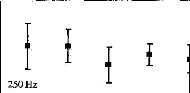
1-4 5-8 9-12 13-16 17-20
Electrode
Figure 49 : Adaptation de sonie
au seuil en pourcentage de la dynamique (par le tone decay test) en
fonction
du site de stimulation (l'électrode 1 est la plus basale,
l'électrode 20 la plus apicale) chez 4
sujets porteurs de l'implant
cochléaire Nucleus. La fréquence de stimulation est de 250 Hz,
l'intensité
mesurée généré un son audible
pendant au moins 60 secondes.
Les résultats obtenus avec les deux types d'implant cochléaire montrent une faible adaptation de sonie lors d'une stimulation électrique continue comparable à celle des normo-entendants.
Cas d'une adaptation de sonie anormale chez un sujet porteur de l'implant cochléaire Nucleus
Nous avons voulu étudier l'adaptation de sonie chez un sujet implanté avec le système Cochlear depuis 3 ans pour lequel nous avons constater ces 12 derniers mois une augmentation progressive suspecte des seuils de détection. L'origine de ce phénomène est probablement due à un dysfonctionnement du système auditif.
La mesure de l'adaptation de sonie au seuil par le tone decay test, nous donne des valeurs moyennes de 83% (d.s. 23%) sur les cinq électrodes actives restantes. Ce genre de cas a déjà été décrit dans la littérature (Brimacombe et Eisenberg, 1984). Ces valeurs bien supérieures aux valeurs précédantes indiquent un dysfonctionnement rétrocochléaire.
b- Fonction de sonie
Des études (Allen et al, 1990) ont évalué la perception de l'intensité ou sonie et son lien avec le niveau du stimulus électrique. La sonie pour une oreille normo-entendante est une fonction puissance du niveau acoustique : L=kPAn. Il est nécessaire de multiplier l'intensité acoustique par 10 pour avoir une sensation de sonie multiplier par 2.
Dans le cas d'une stimulation électrique, la sonie est aussi une fonction puissance du niveau de stimulation électrique mais avec un exposant supérieur. Il est nécessaire de multiplier l'intensité électrique par 2 pour avoir une sensation de sonie multiplier par 2 (Shannon, 1983).
Toutes ces études réalisées chez le sujet porteur d'un implant cochléaire ont utilisé l'amplitude de l'impulsion comme paramètre de codage de l'intensité, hors on sait que cela induit de grande nonliénarité dans le nombre de fibre recrutée en fonction de la stimulation. L'utilisation de la durée de l'impulsion semble être plus appropriée pour coder l'intensité, car elle a l'avantage d'activer toujours la même zone du ganglion avec toujours le même potentiel de fibre.
1- Résolution en intensité
La mesure de sonie est un test difficile a réaliser car il demande une estimation subjective du patient du niveau d'intensité perçu. La mesure du seuil différentiel en intensité est plus communément utilisée car il est plus facile à réaliser. De plus les valeurs mesurées sont très fiables et facilement interprétable.
La mesure de la résolution de sonie se fait généralement par la mesure du seuil différentiel en intensité (IDL). Les sujets implantés cochléaires peuvent détecter un changement de 1 à 2 dB en intensité à proximité du seuil de perception et de 0.25 à 0.5 dB à des intensités plus élevées (Pfingst, 1984 ; Nelson et al, 1996).
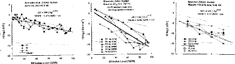
5
Schroder et ai. (1994): Humas AcousUc (300-Ho sine)
4.-E 5
142 -5
F -10
O
-15
-20
-20
100
20 40 60 80
Stimulus Level (%DR)
Shannon (1983), Human Electric (1000-Ha sine) Subi. CE
elfl
· 0.470 ( S.'
18/08)= .0 115 (800) 3.28
O -
11- ELI,2 bp ELSA bp ELI5,18 bp
W1(d9)
E1.1 mp
O ELI5 rnp
5
-15
-20
20 40 60 80 100
Stimulus Level (%DR)
Shannon (1992): Human Electric Wl,,e from TTATFs RI-R5 amplitude modulation
· 82-Na pulsewidtei modulation
PRI e 1.34 ( ).1.37
W7(d0) =-0.188 (813R)
· 1.27
RI mp (sine)
R4 mp (sine)
-
-r-- RS mp (sine)
O N2 bp Wiesel
..6 83 bp (pulse)
Na
bp (pulse)
en o 65 0089
es.7. wr(do). 0 070 (8013)
·1 88
· \A
4 N2 --a-
· N3
Figure 50 : mesure de dl d'après Nelson et al, 1996
Nous avons voulu évaluer, chez 4 sujets implantés cochléaires, les IDL sur l'électrode 5 (basale) et 15 (apicale) pour deux fréquences de stimulation (300 et 1000 Hz) à 4 niveaux de stimulation (10, 30, 70, 90 % de la dynamique).
La technique utilisée pour mesurer le IDL est la méthode adaptative à 'deux intervalles et à choix forcé' (2IFC).
La stimulation se compose de deux trains d'impulsion de 300 ms espacés d'un silence de 500 ms (figure 51). Un train est à une intensité I, l'autre à l'intensité l+dl. La consigne donnée au sujet est d'indiquer le train d'impulsion perçu comme le plus fort. Si le sujet ne trouve pas de différence, il répond au hasard. L'expérience avec une différence en intensité nettement audible (en moyenne dI/1= 0.25). On augmente la valeur du dl dès qu'il y a une erreur. On diminue la valeur dl après 2 réponses justes. Le pas est variable, il diminue de 5 à 0.5 ps. Cette procédure permet de converger vers le seuil à 71%. On calcule ensuite la fonction de Weber 10 log ((l+d1)/1) (I en ps)
dT = 500 ms
I
I+dI
I IIIIIIIIIIIII
|
T=300ms 1 |
.411) T=300ms 2 |
Figure 51: protocole de la mesure de dl. Le train contenant l+dl est de manière aléatoire 1 ou 2.
La figure 52 représente l'évolution de la fonction de Weber (10 log (1+IDL)/1 ) en fonction de l'intensité exprimée en % de la dynamique pour deux électrodes (une basale et une apicale) et deux fréquences de stimulation.
L'analyse statistique de la fonction de Weber par une Anova
à deux facteurs (fréquence, pourcentage
de la_dynamique) sur
des mesures appariées pour les électrodes 5 et 15 donne les
résultats suivants.
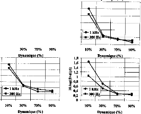
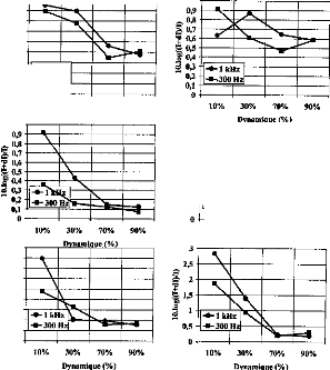
Patient 1
30 %
Patient 2
60%
Patient 3
90 %
Patient 4
80%
Moyenne
65 %
2,5
1,2
|
Electrode 5 |
Electrode 15 |

-6- 1 kHz
- 300 Hz
0
10% 30% 70% 90%
Dynamique (%)
1
1
2,5

-3-j. kHz
-3--31)0
·411z
10% 30% 70% 90%
D nami ue %
g
9:
1,5
d
0,5
1,8
1,6 E 1,4 e 1,2 C.
'e 0,8
a 0,6
"" 0,4
0,2

7 1,5
0,5 -
o
10%
1,4 1,2 1
0,8
e 0,6
0
· ,4
0,2
0
1
g 0,8
C., 0,6
.2%' 1
0,4
0,2
o
0,9
0,8
e0,7 0,6
+ o,5 ' 'g 0,4
· 0,2 0,1
a 0,3
Figure 52: IDL sur 4 sujets
porteurs de l'implant Digisonic en fonction du niveau exprimé
en
pourcentage de la dynamique (10, 30, 70, 90%) pour des fréquences
de stimulation de 300 et 1000 Hz
sur les électrodes 5
(électrode basale) et 15 (électrode apicale). Pour chaque sujet,
les performances
sans lecture labiale de mots triphonémiques sont
indiqués (listes de Lafon)
L'intensité de stimulation a un effet sur la fonction de Weber pour l'électrode 5 (p<0.001) et pour l'électrode 15 (p<0.001). La fonction de Weber diminue lorsque l'intensité de stimulation augmente. Il n'y a pas d'effet de la fréquence pour l'électrode 5 alors que pour l'électrode 15 la fonction de Weber est différente en fonction des fréquences (p<0.001). En effet, l'électrode 15 a une meilleure fonction de Weber à 300 Hz qu'à 1 kHz. Sur l'électrode la plus apicale, le codage de la sonie est donc meilleur pour une fréquence de stimulation de 300 Hz que pour une fréquence de stimulation plus élevée de 1000 Hz.
De manière globale, quelles que soient l'électrode et la fréquence, le IDL décroît lorsque l'intensité de stimulation augmente. La discrimination est meilleure pour les intensités élevées. La forme est comparable à celle obtenue chez le normo-entendants (Tumer et al, 1989). Les valeurs sont identiques voire même plutôt inférieures à celles du normo-entendant. Néanmoins, la dynamique chez le sujet porteur d'un implant cochléaire étant de l'ordre de 8 dB (environ 15 fois moins que pour le normoentendant), le nombre de niveaux de sonie est très inférieur à celui des normo-entendants (environ 15 contre 150 niveaux). Nous avons estimer le nombre de niveaux de sonie à partir de la mesure du dl, sur toute la dynamique électrique. Ces résultats présentés figure 53, en accord avec d'autres études (Pfinsgt et al, 1993; Nelson et al, 1996) effectuées sur d'autres types d'implants cochléaires, montrent un nombre de pas variable suivant le sujet et l'électrode. Il est compris entre 10 et 27.
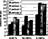
Ill patient 1
patient 2 patient 3
· atient 4
20
18
16
;41 14
o
· 12L 10
8
I 6
4
2
0-50 % 50-100% 0-100%
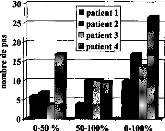
n patient 1
n patient 2 In patient 3
· atient 4
o 10
5
0-50 % 50-100% 0-100%
30
25
ea, 20
0
o 15
Electrode 5 Electrode 15
Figure 53 : nombre de niveaux en
intensité perçue chez 4 sujets implantés
cochléaires pour une
fréquence de 300 Hz sur
l'électrode basale n°5 et apicale n°15
en fonction de la
zone de la dynamique considérée.
Les résultats (fonction de Weber et nombre de pas) sont
différents suivant le patient testé. Le sujet 1 à
une
fonction de weber qui ne décroit pas en fonction du pourcentage de
dynamique. Il correspond aussi
au sujet qui a le plus petit nombre de pas de
sonie (surtout dans la zone 50-100 %). Lorsque l'on
regarde son dossier on s'aperçoit d'une reconnaissance sans lecture labiale médiocre (30%) alors que
celles obtenues par les trois autres sujets testés sont bonnes (sujet 2 : 60% ; sujet 3 : 90% ; sujet 4 : 80%).
Il serait important de confirmer ces résultats par d'autres études plus poussées, car ils suggèrent
- que les caractéristiques individuelles de la fonction de Weber ainsi que le nombre de pas contenu dans la dynamique sont reliés aux performances de reconnaissances du sujet.
- que les fréquences optimales de stimulation permettant de coder la sonie varient en fonction de la zone de cochlée stimulée. Cela pourrait avoir des conséquences sur l'évolution future du traitement du signal de l'implant cochléaire. Actuellement sur la plupart des systèmes d'implants cochléaires, la fréquence de stimulation est fixe ou varie en fonction de la fondamentale laryngée, mais pas en fonction de la zone de la cochlée stimulée.
La mesure systématique du IDL en fonction de l'intensité de stimulation électrique serait intéressant car - elle permettrait de compresser de manière optimale l'énergie acoustique en énergie électrique,
- de choisir un traitement du signal adapté aux caractéristiques du sujet.
Le processeur vocal, doit linéariser le plus possible la discrimination en intensité de la stimulation acoustique en jouant sur la fonction de compression énergie acoustique/ énergie électrique afin d'avoir le même potentiel de discrimination de la parole pour des niveaux d'intensité différents (de 40 à 80 dB SPL).
Afin d'évaluer le système de compression acoustique / électrique actuel, nous avons voulu mesurer chez 8 sujets implantés cochléaires (avec 3 Cochlear : BC, CG, LA et 5 avec Digisonic DE, DU, FA, RO, SC), la discrimination en intensité acoustique avec le traitement du processeur externe. Cela afin d'évaluer sa linéarité pour différentes intensités au-dessus du seuil de détection. 3 niveaux d'intensité acoustique ont été choisis (0, 20 et 40 dB au-dessus du seuil de détection). Ces niveaux correspondent en moyenne à 40, 60 et 80 dB SPL. La fréquence de stimulation acoustique a été fixée à 1000 Hz. Les répartitions fréquentielles des réglages de chaque sujet ont été adaptées pour qu'une seule électrode soit activée (une électrode medium). Avant d'effectuer les mesures de dl, nous avons évalué le seuil de détection par une méthode 2 IFC.
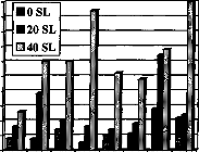
10
9
ee 8
- a 7
eu
= 6 cr
ï 5 =
o 4
te
et 3
1--
"0 2
1
0
DE DU FA RO SC
BC CG LA
Figure 54 : Mesure chez 8 sujets
implantés cochléaires des performances de discrimination
en
intensité d'une stimulation acoustique d'un bruit bande
étroite centré sur 1000 Hz, via le processeur
avec un
réglage correspondant à l'activation une électrode unique
médium.
La figure 54 représente les valeurs de dl observées pour chaque sujet à 3 intensités de stimulation en dB SL. Le dl est variable selon les patients, mais aussi selon le niveau de stimulation (1.32 dB à 0 SL ; 2.63 dB à 20 dB SL ; 6.35 dB à 40 dB SL en moyenne). Le pouvoir de discrimination en intensité décroît lorsque l'intensité acoustique croît quelque soit le système implanté,. Le sujet aura donc plus de difficulté à percevoir des fluctuations en énergie pour des niveaux d'intensité supérieurs à 60 dB SPL.
Quelque-soit le système, la transformation de l'énergie acoustique en énergie électrique n'est pas optimisée pour linéariser la résolution en intensité acoustique.
2- Fonction de sonie
La fonction de sonie chez les sujets porteurs d'un implant cochléaire croit généralement avec l'intensité de stimulation. Sa forme n'est pas toujours linéaire (figure 55) ; elle est dépendante de plusieurs facteurs que l'on ne maîtriser pas parfaitement (étiologie, fréquence de stimulation, fibres recrutées, éloignement entre l'électrode et les neurones...). Lors des réglages effectués au sain de l'hôpital Ed. Herriot, il est même arrivé de voir des patients qui avait au delà d'un certain niveau de simulation une diminution du niveau de sonie.
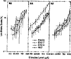
00 400500 700 1000 200 400500 700 1000 300 400500 700 1000
StintlitIS Level (pA)
E20,22 --a E15,17 --t)-
·
E10,12 --e E5,7
Figure 55 : Mesure de la sonie chez 3 sujets 1C, d'après Fu et al, 1998
D'après Zeng et Shannon (1994a,b), la forme et les valeurs de la fonction de sonie se modifient en fonction de la fréquence de stimulation ; ces modifications provoquent des difficultés d'adaptation de l'interface lorsque l'on veut utiliser des stratégies de codages à fréquence de stimulation variable.
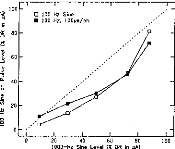
100
.G
c.lr 80
e, 60
a. 40
20
0
100
Figure 56: modèle du
codage de la sonie lors d'une stimulation électrique de la
cochlée
(Zeng et Shannon, 1994b)
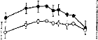
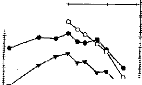

0.1 0.z 0.5
Power fonction exponerrt (P)
--8-- Consonant Recognition --0-- Vondel Recognition
0
50
100
90 A
ôR 80
70
·
80
a
30
cif 20
10 :- 0
au..
60
ct
sa
2')
--e-- Voicing
--O-- Manne
--'e-- Place
Il est important d'évaluer la forme de la fonction de sonie afin d'adapter la fonction adéquat de compression acoustique/électrique. En effet, une étude a montré l'importance de la fonction de compression acoustique électrique sur l'intelligibilité des sujets porteurs de l'implant cochléaire (figure 57). La fonction correspondant à la meilleure intelligibilité est variable selon le sujet testé (Fu et al, 1998).
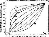
m'Ide Amplitude pat
Figure 57 importance de la
fonction de compression
acoustique / électrique pour le sujet
implanté cochléaire sur
l'intelligibilité,
d'après Fu et al, 1998.
Mesure de la fonction de sonie
Nous avons évalué la fonction de sonie lors d'une stimulation électrique via l'implant cochléaire Digisonic en utilisant la durée de l'impulsion pour coder l'intensité de stimulation. Décrite par Allen et al (1990), la méthode utilisée pour mesurer la fonction de sonie est catégorielle ; après chaque stimulation on demande au patient de classer la force de la sensation perçue parmi plusieurs catégorie (inaudible, très faible, faible, confortable mais faible, confortable, confortable mais fort, fort, très fort, trop fort).
16 sujets implantés cochléaires ont participé à cette étude. Afin d'évaluer l'influence de la fréquence de stimulation et de la zone de cochlée stimulée, trois électrodes (une basale, une médium et une apicale) et quatre fréquences de stimulations (75, 150, 300, 600 Hz) ont été choisies.
Dans un premier temps dans chacune des conditions, les seuils de détection et de confort sont déterminés. 40 niveaux linéairement décomposés de --5% à 105 % de la dynamique électrique sont envoyés au patient de manière aléatoire. Pour chacune des 40 stimulations, le patient juge le niveau sonore parmi les 9 choix précédemment énoncés (de inaudible à trop fort). La fonction de sonie est construite en moyennant les intensités de stimulations perçues pour chacune des 9 catégories.
La figure 58, représente chez 16 sujets testés la fonction de sonie mesurée à une fréquence de 150 Hz sur une électrode apicale. Pour chacun d'eux, on a aussi représenté le pourcentage de reconnaissance sans lecture labiale des listes de mots tri-phonémiques de Lafon.
L'allure de la fonction de sonie ne semble pas dépendante des performances du patient. La fonction de sonie augmente avec la durée de l'impulsion. Au-delà du niveau 'confortable mais fort' le jugement de la sonie sature voir décroît pour certains sujets.
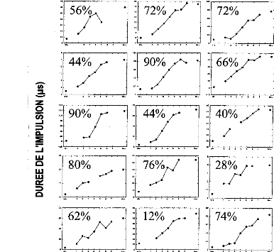
140
120
105
IO
70
20
10
62%
·
/\/
20
10
1.
·
10
U)
|
z |
1 0 |
|
o |
1211 |
|
cn |
100 |
|
110 |
|
|
a. |
00 |
|
2 |
|
|
LU |
24 |
|
CI |
|
|
LU |
20 |
|
lb |
|
|
O |
25
20
10
00
40
30
40% V
10
100
CO
00
IO
00
80%
IO
20
57-4
1 ..... 10.
00
70
05
20
90% /*-.
·
$0
00
|
20 |
Figure 58 Mesures individuelles de la fonction de
sonie pour 16 sujets implantés cochléaires Digisonic
pour une
électrode apicale à une fréquence de stimulation de 150 Hz
et un train d'impulsion de 430 ms.
Chaque niveau de 1 à 7 en abscisse
correspond respectivement à très faible, faible, confortable
mais
faible, confortable, confortable mais fort, fort, très fort.
Pour chaque sujet, on a représenté ses
performances sans
lecture labiale sur les listes de mots tri-phonémiques de
Lafon.
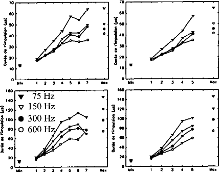
110*
2 3 4 5 6 7
5
1
2
3
4
1110*
5
1
2
3
Mon
4
70
60
50
t 40
30
8
4 20
à
10
o
160
140
3 120
I100
ho -.-
4 60
f 40
j
20
o
;
· -
· 308
3 20
à
10
o
Yin
160
140
1120
.8 n Ina--
I 80
· -
4 60
I0 4 aà
20
o
Yin
i
Min
Yin
1
2 3 4 5 4 7
Mo*
70
60
î 50
140
o
1 2 3 4 5 6 7
110*
Yin
160
1401 120
1100 É80
..-
460
3 à
20
40
Figure 59 : Mesures de la
fonction de sonie pour 16 sujets implanté cochléaires Digisonic
pour différent
sites de stimulation (électrode basale,
médiane, apicale) pour 4 fréquences de stimulation (75, 150,
300
et 600 Hz). Chaque niveau de 1 à 7 en abscisse correspond
respectivement à très faible, faible,
confortable mais faible,
confortable, confortable mais fort, fort, très fort.
La figure 59 représente la moyenne sur les 16 sujets de la fonction de sonie pour différentes fréquences de stimulation et pour différentes zones stimulées. Quelque-soit la fréquence et la zone de stimulation, la fonction de sonie croit avec la durée de l'impulsion. Au-delà du niveau confortable mais fort les fonctions de sonie semblent saturer.
L'analyse statistique par anova à deux facteurs à mesures répétées trouvent des différences entre les niveaux de sonie, mais ne trouve pas de différence entre les catégories confortable mais fort, fort et très fort, cela quelque soit la fréquence de stimulation. Les 3 catégories de sonie les plus élevées sont donc générées par des durées d'impulsion proches.
Il existe un effet de la fréquence sur la fonction de sonie sauf pour la catégorie très faible. Le seuil de détection ne semble pas dépendant de la fréquence de stimulation.
Contrairement à ce qui a été décrit dans la littérature (Zeng & Shannon, 1994), l'allure de la fonction de sonie n'est pas dépendante de la fréquence de stimulation. Du niveau très faible à confortable mais fort, elle semble être linéaire, cela quelque soit la fréquence et le site de la stimulation. L'utilisation d'un traitement du signal à fréquence de stimulation variable est simple avec la stimulation Digisonic. Les seuils de détection sont indépendants de la fréquence et les fonctions de sonie sont linéaires du niveau très faible au niveau confortable mais fort.
3- Equilibre de la sonie en fonction de la fréquence de stimulation
Nous avons voulu affiner les résultats précédants, contradictoires avec ceux de la littérature, par un test plus adapté et beaucoup plus fiable. Plutôt que d'estimer arbitrairement le niveau de sonie, comme le montre la figure 60, ce test consiste à équilibrer en sonie deux trains d'impulsions (un référent et un test).
1 I
11111111 I I
ler Train à F1 2ème Train à F2
Figure 60 : Protocole de la mesure d'équilibre de sonie pour deux trains d'impulsion ayant des
fréquences de stimulation différentes.
Quatre patients ont participés aux mesures qui consistaient à équilibrer la sonie de deux trains d'impulsions ayant des fréquences de stimulations différentes. Deux fréquences de références, 300 et 1000 Hz, ont été choisies pour comparer à 5 fréquences test, 90, 160, 300, 540 et 1000 Hz. Dans chacune des conditions choisies 3 électrodes (une basale, une médiane, une apicale) et quatre niveaux de la dynamiques (10, 30, 70 et 90 %) ont été testés. Dans un premier temps dans chacune des conditions, les seuils de détection et de confort sont déterminés, puis les niveaux à 10, 30, 70 et 90% de la dynamique calculés.
Nous avons utilisé une méthode adaptative (de convergence) avec un pas variable décroissant lors des
quatre premiers changements. La moyenne est calculée en utilisant les 6 dernières alternances parmiles 10 mesurées (figure 61).
SONIE
0 Sonie du deuxième Train
-- Sonie de référence du premier Train
Figure 61: Principe de l'équilibre en sonie pour deux trains d'impulsions.
La figure 62, donne les résultats de la mesure d'équilibre de sonie sur l'électrode 11 pour les différentes conditions chez un sujet. Les valeurs de durée d'impulsion en abscisse et en ordonnée sont en ps. La correspondance de la fonction de sonie pour deux fréquences de stimulation semble très linéaire, ce qui corrobore les résultats concernant l'estimation de la sonie.
|
|
|
|
|
|
||
|
|
||
|
|||
|
|||
|
- 160 Hz - |
- 300 Hz- |
|
O 1 0!0 - 540 Hz o° |
olo _,,, -- go - 300 Hz |
|
0 310 60 90 Hz /_ - |
90 12
|
|
2 310 60 - 300 Hz - qe |
9'O 12 . 1000 Hz - |
|
60 910 12 -1000 Hz- /. / |
|
120 90 60 30 120
je90
eo
O 30
tn
120
90
2 6o
Là
30
0
120
90
e
Cà60
30 120 90 60 O
120 90 60 30
0120 90 60 30
0
o
120
90
60
30
0120 90 60 30
0120 90 60 30
O
o
30 60 90 120 30 60 90 120
Figure 62 : Exemple d'équilibre de sonie sur
l'électrode 11 du patient #2 pour chacune des
conditions
testées. Les valeurs correspondent à la
durée de l'impulsion. Les fréquences de références
sont en
abscisse, les fréquences testées sont en
ordonnée.
Afin d'évaluer la linéarité des équilibres de sonie, on a pour chaque condition testée représenté les valeurs en pourcentage de la dynamique de chaque fréquence de stimulation. Cela nous a permis de regrouper pour chaque patient les valeurs effectuées sur les 3 électrodes testées.
La figure 63 représente les résultats obtenus chez les quatre patients testés dans les différentes conditions. Comme le présente cette figure, les correspondances entre la sonie en fonction de la fréquences de stimulation sont très linéaires, même pour les fréquences basses tel que 90 ou 160 Hz.
Ces résultats montrent que contrairement aux articles de Zeng et Shannon effectués avec les systèmes de Cochlear et Ineraid, l'allure de la fonction de sonie sur le système Digisonic, est indépendante de la fréquence de stimulation dans la gamme 90, 1000 Hz. L'utilisation d'une stratégie de traitement du signal à fréquence de stimulation variable peut facilement être implémentée. Puisque les seuils de détection sont invariants, il suffit d'obtenir la pente de l'équilibre de sonie pour deux fréquences de stimulation différente pour correctement coder la sonie.
|
_ - 90 Hz - .ami- - |
_ __ ... ,,,,..- --; 300 Hz- i i |
|
|
_ - 300 Hz - _ 1 |
1 |
- Hz- 1300 |
|
:1000 Hz |
1 |
300 Hz - 1 |
|
-160 Hz _ _ i |
1 |
- 1000 Hz - i 1 |
|
- 540 Hz - _ |
_ 1000 Hz - |
20 40 60 80 -100
|
- 160 Hz - - :----- ; ------- 1 i |
- - - 300 Hr i i |
|
- 540 Hz i i |
300 Hz- i 1 |
|
90 Hz :,..A 2------ IIII |
1000 Hz- |
|
- 300 Hz - .. III |
1000 Hz- |
|
- 1000 Hz - ../- |
1000 Hz- |
0 20 40 60 80 -100
-100 80 60 40 20
o
-100 80 60 40 20
0
- 100 80 60 40 20
o
- 100
80 60 40 20
o
-100 80 60 40 20
-100 80 60 40 20
o
-100
80 60 40 20
o
-100
80 60 40 20
0
-100
80 60 40 20
o
-100
80 60 40 20
o
o
o
X, Y: %dyn
Figure 63 : Equilibre de la sonie
chez les 4 sujets implantés cochléaires, pour chacune des
conditions
testées en fonction du pourcentage de la dynamique
électrique.
Dans chacune des conditions testées, nous avons mesuré par régression linéaire la pente des équilibres de sonie (fréquence testée, fréquence référante). La figure 64, représente la valeur moyenne de la pente pour chaque condition pour chaque patient testé.
|
Moyenne de la pente 1 .6 1 ,5 300 Hz 1000Hz 1 .4 1 .3 1 ,2 1,0 0,9 0,8 |
90 Hz 160 HZ 300 HZ 540 Hz 1000 Hz
Figure 64 : Pentes moyennes,
calculée par régression linéaire, de la correspondance en
sonie pour
différentes fréquences de stimulation test par
rapport aux fréquences de stimulation référantes 300
et
1000 Hz.
Une comparaison des pentes par rapport à la pente 1 (fonction identité) ne trouve pas de différence statistique pour les conditions 160/300, 300/300, 540/300, 1000/300, 160/1000, 300/1000, 540/1000, 1000/1000 Hz.
Par contre les pentes dans les conditions 90/300 et 90/1000 Hz sont différentes de 1 (p<0.05 pour n=12).
La fonction de sonie diffère donc peu dans la gamme de fréquence de stimulation 160-1000 Hz. La possibilité de faire varier la fréquence de stimulation pour coder une partie de l'information est donc possible avec l'implant Digisonic sans avoir recours à des modifications du réglage.
La résolution temporelle est une propriété majeure de la perception auditive, dans la mesure où la plupart des sons naturels que nous cherchons à percevoir, tels que la parole ou la musique, évoluent dans le temps. Le timbre, la hauteur tonale, la localisation de sources sonores sont autant de propriétés des objets sonores pouvant être comprises sur la base de mécanismes temporels. La résolution temporelle est doublement importante dans la mesure où, très souvent, le bruit masquant en provenance de l'environnement varie en fonction du temps. En lien étroit avec la capacité de démasquage de l'oreille, l'analyse primitive des scènes auditives utilise la cohérence des fluctuations temporelles des composantes sonores afin d'organiser ces dernières en entités sonores ou flux auditifs (Bregman, 1990). Le décodage acoustico-phonétique, l'organisation perceptive de l'environnement sonore et la perception des qualités des sons telles que la hauteur, le timbre ou le rythme dépendent donc étroitement de notre capacité à résoudre des variations temporelles fines.
a- intégration temporelle
L'intégration temporelle mesure le temps au cours duquel, le système auditif intègre l'énergie qu'il reçoit.
Les stimuli de longue durée sont perçus à +
faible intensité a que ceux de plus courte durée. La durée
de stimulation à partir de laquelle le seuil ne change plus est
appelée 'temps d'intégration temporelle'
(TIT). Les sujets
normo-entendants ont des TIT de 100 à 200 ms et paraissent
intégrer la puissance du
stimulus. Quand la durée du stimulus est diminuée de moitié, la puissance du stimulus doit être doublée pour garder le signal à son seuil.
La figure 65 indique les seuils en fonction de la durée du stimulus pour des sujets implantés cochléaires et pour des normo-entendants (Shannon, 1983).Les fonctions sont semblables.
CI Tem oral Inte ration 22 Curve Avera e
|
20 o -0 15 L 10 L -1i 5 O cn 0 |
10 100 1000
Signal Durotion (ms)
Figure 65 Fonction
d'intégration temporelle chez des sujets implantés
cochléaires. La ligne pleine
correspond à celle obtenue
classiquement chez les normo-entendants (Shannon, 1983)).
Nous avons étudié l'intégration temporelle chez sujets implantés cochléaires Digisonic,à différents niveaux de sonie. Nous avons mesuré les fonctions de sonie par mesure catégorielle avec des trains d'impulsions de différentes durées (107, 215 et 430 ms). 12 patients ont été testés sur une électrode apicale à différentes fréquences de stimulation (75, 150, 300 et 600 Hz).
Les résultats, représentés figure 66, montrent des décroissances de la sonie en fonction de la durée de stimulation. Par contre la forme de la fonction de sonie est invariante. Une analyse statistique par Anova à deux facteurs et mesures répétées montre effectivement des différences de la fonction de sonie en fonction de la durée d'impulsion. Par contre les niveaux très faible et faible ne dépendandent pas de la durée.
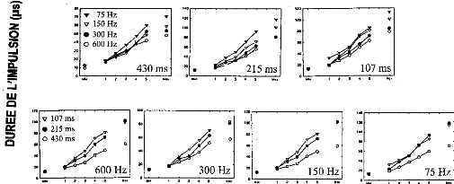
YN
W.
Meg
120
100
40
20
Figure 66 : mesure de la fonction
de sonie par mesure catégorielle chez 12 sujets
implantés
cochléaires en fonction de la durée du train
d'impulsion.
b- résolution temporelle par le 'gap test'
La méthode dite de `gap test' mesure l'aptitude à détecter une brève interruption dans un stimulus continu. En général plus le stimulus est intense, plus le seuil de détection de l'interruption est cours. Les sujets implantés cochléaires ont les mêmes performances que les sujets mormo-entendants (Moore et al, 1988).
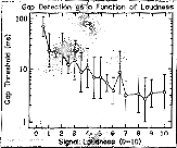
Gap Detection as c Funcflon of Lou
Figure 67 : Résolution
temporelle avec le gap test en
fonction du niveau de sonie, d'après
Shannon 1983
Mesure de la résolution temporelle par le 'Gap test'
Nous avons évalué la résolution temporelle (gap) sur une électrode apicale pour deux fréquences de stimulation (300 et 1000 Hz) à 4 niveaux d'intensité de stimulation (10, 30, 70, 90 % de la dynamique).
Comme le montre la figure 68, l'expérience consiste à enlever des impulsions (de 0 à 20) au milieu d'un train de 200 impulsions (0.66 seconde pour la fréquence 300 Hz, 0.20 seconde pour la fréquence 1000 Hz) et de demander au sujet testé s'il perçoit un son ou deux sons. Le gap est présent de manière aléatoire (p=50%) et toujours égal à un multiple de la période de stimulation. En effet un gap d'une durée ne correspondant pas à un multiple de la période pourrait être détecté par déphasage entre les deux trains d'impulsions. On commence avec 20 impulsions supprimées, puis on diminue en fonction de la réponse du sujet, jusqu'à ce que l'on converge vers un nombre d'impulsions enlevées à la limite de la perception du gap. La technique utilisée pour converger vers la valeur limite est une procédure 2 IFC (décrite pour la mesure du dl). On transcrit ensuite le nombre d'impulsions en millisecondes (x3.3 pour f=300 Hz, x1 pour f=1000 Hz).
dT (= k / F)
|
T=300ms |
|
|
T=300ms |
Figure 68 : protocole de la
mesure de résolution temporelle (gap test). K est le nombre
d'impulsions
enlevées. F est la fréquence de stimulation du
train de 200 impulsions.
La figure 69 représente l'évolution de la résolution temporelle en fonction des niveaux de stimulation (en pourcentage de la dynamique) pour deux fréquences de stimulation (300 et 1000 Hz). La forme des courbes est de type exponentiel décroissant. Les meilleurs seuils sont obtenus à des intensités de stimulations fortes. Ces résultats sont comparables a ceux obtenus avec d'autres systèmes d'implant cochléaire (Shannon, 1983, 1989). Ils sont aussi comparables à ceux obtenus chez les normoentendants (Moore et Glasberg, 1988). Le gap semble être stable à partir de 30 % de la dynamique. Les capacités de résolution temporelle des sujets porteurs d'implant cochléaire sont les mêmes que celles des sujets normo-entendants. Les 5 sujets testés peuvent percevoir l'absence d'une impulsion dans un train de 200 impulsions à 300 Hz pour des intensités de stimulation de 70 et/ou 90 % de la dynamique.
L'analyse par Anova montre une dépendance du gap au pourcentage de la dynamique (p<0.001) et une indépendance à la fréquence de stimulation. Le seuil à 10 % de la dynamique est différent des seuils à 30, 70, 90 % de la dynamique. Cela peut facilement s'expliquer physiologiquement. En effet, à faible niveau d'intensité perçue, le nombre de fibres recrutées et la synchronisation des fibres sont plus
faibles. La période réfractaire du groupe de neurone est plus longue et la synchronisation moins importante. La résolution temporelle est par conséquent moins bonne. La résolution temporelle ne semble pas être dépendante de la fréquence de stimulation. Par contre, on peut constater que les deux patients qui ont les meilleures résolutions temporelles sont les deux meilleurs patients.
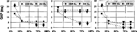
100% 0%
25% 50% 75%
0% 25% 50% 75%
25
7i 20
E
15
a.
<
0 io
5
0
|
|
||||
|
|||||
|
|
||||
|
|||||
|
|||||
z
t
-*
25% 50% 75% 100%
o
100% 0%
4....
5
4
3
2
25
20
15
10
5
· - 1000 Hz -
· - 300 Hz'
- 4- 1000 Hz - - 300 Hz
s.
· -
- - -
·
|
|
|||||||||
|
||||||||||
|
|
|||||||||
|
||||||||||
|
|
|
||||||||
|
|
|||||||||
Patient 3 : 30 %
|
|
|||||
|
||||||
|
||||||
|
|
|
||||
75% 100%
25 20 15 10 5 0
70
60
1/7 50
· 40
· 30
20
10
0
0%
25% 50% 75% 100% 0% 25% 50% 75% 100% 0% 25% 50%
Patient 4 : 60 % Patient 5 : 80 % Moyenne : 59 %
Figure 69 : Résolution
temporelle (Gap en ms) sur 5 sujets porteurs de l'implant Digisonic en
fonction
de différents pourcentages de la dynamique (10, 30, 70, 90)
pour des fréquences de stimulation de 300
et 1000 Hz sur une
électrode apicale. Les flèches indiquent des limites de la mesure
(vers le haut : cela
correspond à une valeur sous estimée ;
vers le bas cela correspond à une valeur sur estimée).
Pour
chaque sujet testé, on a indiqué ses performances sans
lecture labiale sur une liste de mots
triphonémique de Lafon.
La résolution temporelle étant très déterminante pour la reconnaissance de la parole chez le sujet porteur de l'implant cochléaire (Cazal et al, 1991, 1994), la question est de savoir s'il faut supprimer la première partie de la dynamique pour coder l'information pour ne garder que la partie 30-100 % de la dynamique ? Cette question parait intéressante à élucider car elle permettrait peut-être d'améliorer les performances des sujets porteurs d'implant cochléaire pour des niveaux acoustiques faibles. Une étude plus exhaustive sur l'influence de la partie de la dynamique électrique utilisée sur les performances parait donc intéressante.
c- Les modulations en amplitude
L'organisation perceptive de l'environnement sonore, la perception du timbre des sons et l'intelligibilité de la parole dépendent étroitement de la capacité du système auditif à résoudre les variations temporelles lentes de l'amplitude des sons, i.e., l'enveloppe temporelle des sons.
Les caractéristiques acoustiques de l'enveloppe, telles que l'intensité, le temps de montée, le temps de descente, et la fréquence de fluctuation déterminent respectivement les sensations de force, d'attaque, de chute, de rugosité et de tempo. La forme de l'enveloppe temporelle est également impliquée dans la perception du timbre et dans les processus de reconnaissance d'objets sonores.
La mesure de la sensibilité auditive d'un patient aux fluctuations est directement reliée à l'acuité (ou la résolution) temporelle du système auditif. Une description plus complète de la résolution temporelle du système auditif peut être réalisée en mesurant la fonction de transfert de modulation temporelle (TMTF, pour Temporal Modulation Transfer Function). Dans ce test psychoacoustique (Viemeister, 1979), les stimuli sont des bruits large bande modulés sinusoïdalement en amplitude à une fréquence donnée. La TMTF relie la performance de déduction de la modulation d'amplitude à la fréquence de modulation. La performance (ou le seuil) de détection de la modulation d'amplitude, mesurée en décibels (20 log(m)), correspond à la plus petite profondeur de la modulation d'amplitude, m, permettant de juste discriminer un bruit non modulé. Les TMTFs obtenues par Viemeister (1979) présentent une caractéristique passe- bas : la performance de détection est constante jusqu'à environ 8 Hz. Elle se réduit de 3dB à environ 50 Hz, puis elle décroît de manière monotone de 3-4 dB/octave (on parle de 'pente d'atténuation') jusqu'à approximativement 800 Hz. .30
-25
-20
-10
-5
2 8 16 32 64 125 250 500 1000 2000 9000"0
Figure 70 : Fonction de transfert
de modulation d'amplitude (TMTF) mesurées chez quatre sujets.
La
porteuse est un bruit large bande. D'après Viemeister,
1979,
Bien que la résolution en fréquence et en intensité chez le sujet porteur d'un implant cochléaire est très appauvrie en comparaison à celles du normo-entendant, elle est suffisante pour coder les modulations (Shannon, 1991 ; Cazal et al, 1994). Cela s'explique principalement par la très bonne résolution temporelle précédemment décrite des sujets porteurs d'un implant cochléaire (Shannon, 1983, 1989 ; Cazal et al, 1991). Les TMTFs obtenues chez des patients porteurs d'un implant cochléaire (Shannon, 1992) sont également similaires à celles obtenues chez des sujets normo-entendants (Shannon, 1992 ;
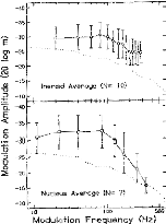
E
cf) -
o
VV
E
o
u
C1
Nucleus Average (N= 7)
iou
ciulation Frequency (Hz)
Ineraid Average (N= 10)
Kohlrausch, 1993).
Figure 71: mesure de la fonction de transfert
de
modulation d'amplitude chez sujets implantés
cochléaires
(Inaired ou Nucleus) comparé au
normo-
entendant, d'après Shannon
1992
Des travaux (Shannon et al, 1995) ont montré la possibilité de coder la parole avec des indices d'enveloppe du signal ; les résultats sont fonction du nombre de canaux fréquentiels utilisés, mais aussi des fonction de compression entrée sortie (Fu et al, 1998).
Enveloppe et compression
S. Gallégo
Proceeding du congrès de la
société française d'Audiologie, Clermont-Ferrand,
déc 1998
Sous presse
L'objectif de cet article a été double :
Nous avons voulu montrer qu'il était possible de reconnaître de la parole par l'enveloppe du signal acoustique. Les résultats montrent qu'avec simplement 4 canaux laissant passer l'enveloppe jusqu'à 250 Hz, il est possible de reconnaître plus de 80% des phonèmes,
Nous avons voulu montrer qu'avec un type de compression fondée sur l'enveloppe et n'utilisant pas les temps d'attaque et de retour, il est possible de ne pas détériorer l'intelligibilité.
Préservation de l'enveloppe temporelle pour la compression du signal de parole.
Stéphane Gallégo
Laboratoire CNRS UPRESSA 5020, Lyon
Laboratoires MXM,
Vallauris
Centres GAM surdité, Mougins
e-mail :
sgallecioemxmlab.com
Introduction : La perception des fluctuations d'amplitude lentes joue un rôle certain dans la délimitation des unités linguistiques (voyelles, syllabes ou mots). Ces fluctuations d'enveloppe sont également impliquées dans plusieurs distinctions phonétiques importantes. Plusieurs études ont montré que la reconnaissance des signaux de parole pouvait être effectuée sur la base des indices d'enveloppe temporelle. Katz et Berry (1971), Van Tassel et al (1987), et plus récemment Shannon (1995) ont obtenu d'excellents scores d'intelligibilité de la parole en modulant des bruits blancs ou des bandes de bruits par l'enveloppe de signaux de parole (figure 1).
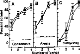
2 3 4 1 2 3 4 1 2 3 4 Nimber of bands
Figure 1: Reconnaissance des consonnes, voyelles et phrases chez huit sujets normoentendants en fonction du nombre de bandes de bruits filtrés à la place de la structure fine du signal après environ 10h d'apprentissage. D'après Shannon et al, 1995
Les bonnes performances d'intelligibilité de la parole obtenues chez des sujets porteurs d'implants cochléaires mono-électrodes (Hochmair et Hochmair-Desoyer, 1985) ou du système percutané lnaired à quatre canaux (Dorman et al, 1990) témoignent également de l'importance des indices d'enveloppe dans la compréhension de la parole. Des études (Lawson, Wilson et Finley, 1992), montrent que l'intelligibilité chez les sujets porteurs de l'implant cochléaire lnaired est fonction du nombre de canaux actifs. Avec six canaux, le score est proche du sans faute. Des études chez le normo-entendant, principalement investiguées par l'équipe de Drullman (Noordhoek & Drullman, 1997) ont caractérisé la perte d'intelligibilité en fonction de la dégradation de l'enveloppe temporelle des mots. Les résultats montrent que l'information est principalement contenue dans les fréquences comprises entre 1 à 32 Hz. Plus le spectre de l'enveloppe est réduit plus l'intelligibilité est faible.
Les résultats obtenus chez des patients présentant une surdité sensorineurale par stimulation acoustique (Bacon & Viemeister, 1985 ; Moore, Shailer & Shooneveldt, 1992 ; Lorenzi et al, 1997, Demany et Lacher-Fougère, 1997) ou électrique (Shannon, 1992, Kohlrausch, 1993) sont similaires à ceux obtenus chez des sujets normo-entendants. Ces Résultats montrent que le mécanisme responsable de l'intégration temporelle des sons (et de l'extraction de l'enveloppe) n'est pas affecté par une atteinte cochléaire. Ils suggèrent donc que ce mécanisme se situe à un niveau central (rétro- cochléaire) plutôt que périphérique (cochléaire).
Expérience 1 : Nous avons voulu
évaluer l'importance de l'enveloppe de la parole en éliminant
toute la
structure fine du signal. Ce genre de traitement peut
présenter un intérêt pour les surdités ayant
une
forte dégradation de la sélectivité
fréquentielle, seul le facteur temporel intervient dans ce genre de
test
(par exemple les surdités profondes ou sévères ont une tonotopie cochléaire très frustre, seules les caractéristiques temporelles du signal peuvent être codées).
Son principe de base est de garder l'enveloppe du signal pour différents canaux (1 à 4) et de remplacer la structure fine de chaque canal par un bruit passe-bande équilibré en énergie (figure 2).
Contrairement aux travaux de Shannon (1995), nous ne voulons pas qu'il y ait une séance d'entraînement longue qui permet d'améliorer les scores de reconnaissance (8 à 10 heures par sujet testé). Cela permet, d'éviter un recodage des sons. L'expérience sans entraînement permet de mesurer l'intelligibilité correspondant à celle obtenue par un traitement de la voix la plus naturelle possible.
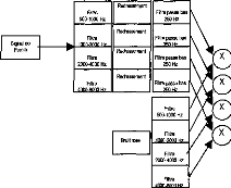
Filtre
500-1000 Hz
Filtre passe bas
250 Hz
Redressement
Filtre
1000 .2000 H7
Filtre
2000-4000 Hz
Filtre
eoneloo H7
Redressement
Redressement
Redressement
Bruit rose
Filtre
2000-4000 Hz
Signal de
Parole
Signal
Traité
Figure 2 : Schéma simplifié du traitement de signal effectué pour remplacer les structures fines de chaque canal par un bruit rose filtré.
Nous avons choisi les listes de mots utilisées classiquement en cabinet d'audioprothèse pour mesurer l'intelligibilité. Ce sont 40 listes de 10 mots dissyllabiques numérisées sur CD ROM, elles ont été élaborées par monsieur Fournier. Pour chaque mot deux mesures d'intelligibilité ont été effectuées : 1- la reconnaissance du mot (0 ou 100%), 2- le pourcentage de phonèmes reconnus dans les mots (de 0 à 100%).
Pour chaque sujet testé nous avons passé deux listes par condition sur l'oreille droite. L'intensité de stimulation est à environ 30 dB SL. Quatre conditions dans un ordre aléatoire ont été choisies ( un canal (2000-4000 Hz) ; 2 canaux (1000-2000, 2000-4000 Hz) ; 3 canaux (1000-2000, 2000-4000, 4000-8000 Hz) ; 4 canaux (500-1000, 1000-2000, 2000-4000, 4000-8000 Hz)).
Figure 3 : Pourcentage et déviation standard de phonèmes reconnus (graphe de gauche) et pourcentage et déviation standard de mots reconnus (graphe de droite) en fonction du nombre de canaux pour une population de 20 normo-entendants.
100 100 - - -
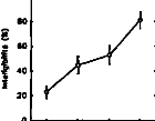
20
80
60
14 40
3
20
1 2 3 4
Nombre de tonere

Nombre de «noue
Les mots et phonèmes sont très bien reconnus par les normo-entendants (90 % pour les mots et 95 % pour les phonèmes chez certains sujets). Les résultats sont similaires à ceux décrit par Shannon et al, 1995, mais dans ses conditions expérimentales, il y avait un entraînement au préalable d'une dizaine d'heures. Ces résultats corroborent aussi ceux de Lawson et al, 1992 obtenus chez les sujets implantés cochléaires. L'intelligibilité (des mots et des phonèmes) croit en fonction du nombre de canaux. Une analyse statistique par Anova montre des différences statistiques de performances en fonction du
nombre de canaux utilisés (p<0.001 : 43, 42, 41, 32, 32, 21). Les résultats montrent qu'un système auditif qui peut faire la différence entre quatre fréquences et qui a une résolution temporelle normale peut avoir un intelligibilité d'environ 95 % sans qu'il soit besoin de recoder l'information auditive sous une forme différente. Cela peut en partie expliquer les performances obtenues chez certains enfants sourds profonds utilisant la prothèse à transposition de fréquence de Lafon (Lafon, 1996).
L'utilisation de l'enveloppe chez les sujets atteints d'une surdité de perception est actuellement mal adaptée avec les appareils conventionnels. Lorsque l'on adapte l'énergie acoustique par une aide auditive au sujet atteint d'une surdité de perception, on utilise actuellement des systèmes de compression qui ont des seuils de déclenchement avec des temps d'attaque et de retour variables. Cela entraîne évidemment des distorsions de l'enveloppe temporelle du signal en dynamique Une compression qui permettrait de ne pas déformer l'enveloppe tout en préservant le spectre fréquentiel instantané serait sûrement plus avantageuse.
Expérience 2 : L'expérience précédante a montré l'importance de l'enveloppe sur l'intelligibilité et a soulevé le problème de distorsion de l'enveloppe lors de la compression du signal dans les aides auditives actuelles. Nous avons ensuite voulu estimer les performances d'un type de compression ou d'extension du signal de la parole. Des tests d'intelligibilité dans le bruit ont été choisis pour évaluer la qualité de la compression. La technique utilisée pour compresser ou étendre le signal se base sur la modification de l'enveloppe temporelle en préservant sa forme et la structure spectrale du signal. L'avantage de ce type de technique est d'éliminer tout effet indésirable de distorsion lorsque le signal n'est pas stationnaire.
Lorsqu'un sujet a un recrutement important, il est intéressant d'utiliser cette technique de compression car elle préserve la structure fine et la forme de l'enveloppe du signal. Moore, 1992 montre que pour simuler une surdité avec une audition normale (surdité de perception) l'enveloppe du signal doit être comprimée par sa racine carrée (compression de 1/2).
L'objectif du traitement du signal est de préserver le spectre instantané et la forme de l'enveloppe temporelle du signal lors d'une compression. Il est donc nécessaire d'extraire séparément l'enveloppe et la structure fine du signal, puis de compresser uniquement l'enveloppe.
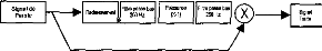
Puissance
(X-'1)
Redressement
Filtre passe bas
250 Hz
Signal de
Parole
29
Filtre passe bas __H
250 Hz
Signal
Traité
Figure 4 : Schéma simplifié du traitement de signal effectué pour compresser l'enveloppe du signal bruité. Si l'on veut compresser par 1/2 la puissance sera --1/2.
Pour chaque sujet testé nous avons passé une liste par condition sur l'oreille droite. L'intensité de stimulation est à environ 30 dB SL. Pour chaque sujet six types de compressions avec quatre rapports signal sur bruit ont été choisis ( compression de 1/8, 1/4, 1/2, 1 et expansion de 2 et 4 ; rapport signal sur bruit de 12, 6, 0 et-6 dB).
L'exemple figure 5 nous montre que le fait de compresser un signal diminue le rapport signal sur bruit. Inversement une extension du signal augmente le rapport signal sur bruit. Malgré cela les résultats figure 5 ne montrent pas de différence statistique (par une anova à deux facteurs à mesure répétée) de l'intelligibilité en fonction du facteur de compression (ou d'extension). Ce type de compression ne modifie apparemment pas l'intelligibilité dans le bruit. Comme nous nous y attendions, le traitement du signal utilisé permet de préserver la forme de l'enveloppe ainsi que les structures fines du signal, ce qui se traduit par la stabilité de la compréhension de la parole dans le bruit.
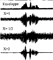
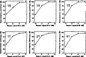
gee
laa
g ion
ew
RO
g
°
"
I4°
10
40
-à 0 6 12
ROmMari mienOlibrue (104
40
110
-6 0 12
mignml/bre idlj
-fi 0 12
%neer! 0ignaV0re {dol
6 0 12
%oued eigned/brun {dl]
-a 0
Re9mor1 161/.01/11/0e
Il tee 60 RO 40
1
-Il 0 6 12
nomplaigne/bnall tai
Î 100
"
40
110
a 100 I MO I 40 I 40
I20
0
Figure 5 : Exemple du traitement de signal pour le mots 'le bouchon' pour les différents taux de compression X (gauche); Intelligibilité des phonèmes pour différentes compressions à différents rapports signal sur bruit sur une population de 20 sujets (droite).
Bien qu'artificiellement le rapport signal sur bruit se dégrade lors d'une compression (figure 5), l'intelligibilité reste identique. L'utilisation de ce type de traitement semble être intéressant pour les aides auditives par rapport aux compressions utilisées actuellement.
Afin de valider ce type de compression, il semble intéressant de poursuivre ces investigations sur des sujets atteints d'une surdité de perception. Plusieurs sous-groupes, en fonction du niveau de surdité, doivent être étudiés (de la surdité moyenne à profonde).
Bibliographie :
Bacon SP, Veimeister NF. Temporal modulation transfer functions in nomal-hearing and hearing impaired subjects. Audiology, 1985, 24,117-134
Demany L, Lacher-Fougère S. Consequences des pathologies cochléaires sur la perception des modulations sonores. Cahier de l'audition, 1997, 10, 3; 15-17
Dorman MF, Soli S, Dankowski K, Smith L, McCandless G, Parkin J. Acoustic cues for consonant identification by patients using Inaired cochlear implant. J Acous Soc Am, 1990, 88, 2074-2079
Hochmair-Desoyer IJ, Hochmair ES, Stiglbrunner HK. Psychoacoustic temporal processing and speech understanding in cochlear implants patients. In RA Schindler & MM Merzenich (Eds), Cochlear implants, New York :Raven Press, 1985, 291394
Katz SJ, Berry RC. Speech modulated noise. 81nd Meeting of Acoustical Society of America, 1971.
Kohlrausch A. Comment on 'Temporal modulation transfer functions in patients with cochlear imlants'. J Acous Soc Am, 1993, 93, 1649-1650
Lafon J.C. Transposition et modulation pour que les sourds entendent. Bull. Audiophonologie, 1996, 12, 3&4
Lorenzi C, Micheyl C, Berthommier F, Portalier S. Modulation masking in listeners with sensorineural hearing Ioss. J Speech & Hear Res, 1997, 40, 200-207
Lawson DT, Wilson BS, Finley CC. New processing strategies for multichannel cochlear protheseses. Progress in brain research, 1992.
Moore BJC, Shailer MJ, Schooneveldt GP . Temporal modulation transfer functions for band-limited noise in subjects with cochlear hearing loss. Brit J Audiol, 1992, 26, 229-237
Noordhoek IM, Drullman R. Effect of temporal intensity modulations on sentence intelligibility. J Acous Soc Am, 1997, 101, 498-502
Shannon RV, Zeng FG, Kamath V, Wygonski J, Ekelid M. Speech recognition with primarily temporal cues. Science, 1995, 270, 303-304
Shannon RV. Temporal modulation transfer functions in patients with cochlear implants. J Acous Soc Am, 1992, 91, 21562164
Tasell D Van, Solli SD, Kirby VM, Widin GP. Speech waveform envelope cues for consonant recogniton. J Acous Soc Am, 1987, 82, 1152-1161
Discrimination d'enveloppe
Les caractéristiques acoustiques de l'enveloppe, telles que l'intensité, le temps de montée, le temps de descente, et la fréquence de fluctuation déterminent respectivement les sensations de force, d'attaque, de chute, de rugosité et de tempo. La forme de l'enveloppe temporelle est également impliquée dans la perception du timbre et dans les processus de reconnaissance d'objets sonores. Une note de piano, par exemple, possède une attaque rapide et une chute relativement lente. Cette même note enregistrée sur une bande puis écoutée en sens inverse change de timbre et évoque celui d'un accordéon. Cet effet souligne bien l'importance des indices temporels dans la perception du timbre car les spectres de puissance des versions 'avant' et 'arrière' du signal sont identiques.
Des travaux portant sur la mesure de l'activation des zones corticales avec une stimulation sonore ont montré que le traitement cortical d'un signal de parole était très différent des versions 'avant' et 'arrière'. Le signal de parole émis à l'envers (par rapport au temps) n'était pas traité par le cerveau comme un signal de parole.
La mesure de la TMTF semble donc insuffisante pour évaluer les capacités des sujets implantés à analyser l'enveloppe du signal.
J. Acous. Soc. AM., 1997, 102(1), 482-485
L'objectif de cette étude a été d'évaluer sur une population de 5 sujets implantés cochléaires Digisonic, leur capacité de discrimination deux enveloppes temporellement asymétriques. Les signaux utilisés dérivent de l'étude de Patterson et al, 1994 effectuée chez les normo-entendants et sont directement transmis au récepteur interne via l'antenne sans passer par le processeur vocal.
Les résultats montrent que les sujets implantés discriminent mieux les asymétries temporelles du signal que les sujets normo-entendants. Cela pourrait être expliqué par l'absence de lissage due à la biomécanique cochléaire lors d'une stimulation électrique.
Discrimination of temporal asymmetry in cochlear implantees
Christian Lorenzi
MRC, Applied Psychology Unit, 15 Chaucer Road, Cambridge CB2 2EF, United Kingdom and PCH Département de Psychologie Cognitive, Institut de Psychologie, Université Lumière Lyon II,
69676 Bron Cedex, France
Stéphane Gallego
Laboratoire de Physiologie Sensorielle, "Perception & Mécanismes Auditifs," UPRESA CNRS 5020, Pav. U. Hôpital E. Herriot, 69437 Lyon Cedex 03, France
Roy D. Patterson
MRC, Applied Psychology Unit, 15 Chaucer Road, Cambridge CB2 2EF, United Kingdom
(Received 1 February 1996; revised 2 January 1997; accepted 2 April 1997)
Several studies have recently demonstrated that normal-hearing listeners are sensitive to short-term temporal asymmetry in the envelopes of sinusoidal or noise carriers. This paper presents a study in which cochlear implantees were presented trains of current pulses with temporally asymmetric envelopes through one channel of an implant that stimulates the auditory nerve directly, thereby bypassing cochlear processes. When the level of the stimuli was adjusted to fit their audibility range, the implantees were able to discriminate temporal asymmetry over a much wider range than normal-hearing listeners. The results suggest that the perception of temporal asymmetry is limited by compression in the normal cochlea. (c) 1997 Acoustical Society of America. [S0001-4966(97)06707-6]
PACS numbers: 43.66.Jh, 43.66.Mk, 43.66.Sr, 43.66.Ts [WJ]
INTRODUCTION
When a sound with an asymmetric temporal envelope is reversed in time, it often produces a marked change in the timbre of the sound. The effect is important because the power spectrum of a sound does not vary with the time reversai. Although the perceptual effect of the time reversai is well-known, it was largely ignored until recently, when Patterson (1994a, b) showed how the effects of the time reversai could be studied systematically using "damped" and "ramped" sinusoids. The term "damped sinusoid" refers to a segment of a sinusoid with a damped exponential envelope that is repeated cyclically to produce a sustained sound. The "ramped sinusoid" is simply the damped sinusoid reversed in time. The envelope "damps" down in the former case and "ramps" up in the latter case. Normal-hearing listeners can discriminate damped sinusoids from ramped sinusoids when the half-life of the envelope is in the range 1-50 ms. Compression in the cochlea of the normal-hearing listener reduces the dynamic range of damped and ramped sinusoids in the neural representations flowing from the cochlea. This led to the intriguing suggestion that cochlear implantees might exhiba even better asymmetry discrimination than normalhearing listeners because the implant bypasses the cochlea and any compression it might impose. We assume, as argued by Shannon (1986), that sensitivity to level differences in the central auditory system of cochlear implantees is about the same as that for normals when presented at the same sensation level. It is also the case that with implantees, one can restrict the stimulation to a single electrode and thereby preclude spectral cues to a degree that is not possible with normal listeners. Thus cochlear implantees would appear to pro- vide us with a unique opportunity to investigate the limits of retrocochlear processing of temporal asymmetry.
There have been several demonstrations that cochlear implantees can process temporal envelope information. Hochmair and Hochmair-Desoyer (1984) reported that implantees could distinguish among square, triangle, and sine waves for repetition frequencies up to 400 Hz. Shannon (1986) demonstrated near normal temporal integration, gap detection, and forward masking in two implantees, and more recently, Shannon (1992) reported that implantees could detect amplitude modulation at least as well as normal-hearing listeners. In these experiments, however, there is no manipulation of temporal asymmetry.
I. EXPERIMENT
Pairs of ramped and damped envelopes with the same half-life were presented to cochlear implantees to assess their discrimination of temporal asymmetry. The electrical signal was delivered directly to a single electrode of a Digisonic DX10 implant without going through the preprocessor to avoid the compression normally applied by the device.
A. Method
Five postlingually deaf listeners (SP, BM, LR, FJ, BR) participated in the experiment. Clinical information about these patients is presented in Table I. They were ail implanted with a Digisonic DX10 device (MXM), which is a transcutaneous 15-channel cochlear implant with an intracochlear electrode array (Beliaeff et al., 1994). Activation was limited to the most basal electrode which delivered biphasic current pulses; the remaining 14 electrodes in the array were connected together to serve as the return path for the current
|
Age Patient (years) |
Cause |
Duration of |
Pulse amplitude (V) |
Min Max (us/phase) (,us/phase) |
2 a C |
||
|
BM |
64 |
head trauma |
7 |
1.5 |
12 |
55 |
|
|
SP |
44 |
head trauma |
6 |
1.3 |
14.5 |
45 |
|
|
LR |
60 |
unknown |
3 |
1.3 |
10 |
45 |
|
|
FJ |
45 |
head trauma |
48 |
1.6 |
25 |
95 |
|
|
BR |
36 |
progressive deafness |
1 |
1.3 |
10 |
40 |
ri a |
|
C o o |
|||||||
TABLE I. Clinical data for the five cochlear implantees of the study.
("common ground" mode of stimulation). X-ray photographs revealed that electrode positioning was roughly the same for all implantees. All stimuli were presented directly to the implanted electrode without going through the speech processor. For each implantee, the pulse amplitude was fixed and the pulse duration was adjusted from threshold (min) to comfort level (max); the pulse amplitude and the min and max values for each implantee are presented in Table I. All implantees were experienced in two-interval, two-alternative forced choice tasks (21, 2AFC).
1. Stimuli
The stimuli were trains of biphasic current pulses of fixed amplitude. The pulse duration as a function of time was shaped by a ramped or damped function. Equation (1) shows the general foret of a damped envelope:
damp( t )= min + [max -- min]exp[c t/h1] ( 0 < t < T),
(1)
hl is the half-life of the damped envelope, and c is a constant (-0.693 147), that brings the envelope to [max --Inin]/2 in hl ms. T is the repetition period which is 50 ms. The pulse rate was 800 Hz, which was the maximum pulse rate provided by the device used to perform direct stimulation. The ramped envelopes were produced by reversing the damped envelopes in time. The envelopes were digitally generated on a PC by a 16-bit D/A converter at a sampling frequency of 44.1 kHz. The electrical stimuli were generated using a Digistim system (MXM) connected to the PC via a serial port. The duration of the stimuli was 500 ms; the silent interval between stimuli was 500 ms. The comfort level, max, was adjusted as the half-life was increased so that the stimuli were of approximately equal loudness. The loudness of the stimuli was equated by asking each implantee to adjust the level of each damped stimulus to that of a damped stimulus with a 8-ms half-life. Adjustment was performed using an initial step size
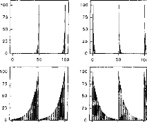
0
o
10
50
10
100
75 -
50
25 -
11111111..,.
100
75
50
25
0
100 75 50 25
o
lÎ
L IL
100
75
50
25
0 rmeitil
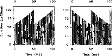
o
50
100
o
5
100
0 50
Time (ms)
100
î 100
g 75
C
uc=, 50
0 25
o
FIG. 1. Ramped (left column) and damped (right column) current pulse trains with a half-life of 1 ms (top section), 8 ms (middle section), and 64 ms (bottom section). The carrier frequency is 800 Hz. The repetition period is 50 ms.
of 5us/phase and a final step size of 0.5 ,us/phase. Three estimates were collected and averaged. The average max values measured for each half-life and for each implantee are presented in Table II.
Segments of the current pulse trains are presented in Fig. 1; the left and right panels show ramped and damped fonctions, respectively. The half-life of the exponential is 1 ms in the top section, 8 ms in the middle section, and 64 ms in the bottom section of Fig. 1. The trains of current pulses show that the Digistim system preserves the temporal envelope.
2. Procedure
Implantees sat in front of a keyboard connected to the computer controlling the experiment. The task was 21, 2AFC. In a given trial, implantees were presented a ramped stimulus in one interval and a damped stimulus with the same half-life in the other interval, and asked to choose the interval with the "more tonal quality." In each trial, inter-
TABLE II. Max values (in ms/phase) producing stimuli of equal loudness as the half-life is increased from 0.25 to 1024 ms. The data are presented for the five cochlear implantees of the study.
|
hl |
0.25 |
0.5 |
1 |
2 |
4 |
16 |
32 |
64 |
128 |
256 |
512 |
1024 |
|
BM |
65 |
60 |
60 |
60 |
55 |
55 |
50 |
45 |
40 |
40 |
37 |
40 |
|
SP |
53 |
52.5 |
50 |
48 |
46.5 |
44 |
43 |
42 |
41 |
40 |
38 |
37.5 |
|
LR |
38 |
40 |
41 |
43 |
45 |
45 |
45 |
45 |
40 |
37 |
35 |
35 |
|
FI |
80 |
86.5 |
90 |
90 |
95 |
95 |
85 |
77 |
71 |
65.5 |
67 |
65 |
|
BR |
35 |
35 |
35 |
37 |
42.5 |
36 |
31.5 |
30 |
27.5 |
23 |
23 |
23 |
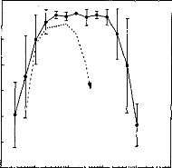
100
90
80
8
.g 70 2
60
50
40
0.1 10 100 1000 10000
Half-life (ms)
FIG. 2. Average psychometric function for the five cochlear implantees, showing performance as a function of hl. Error bars show one standard deviation about the mean performance of the five implantees. For comparison, the data are piotted along with the mean of the data obtained with normal-hearing listeners.
vals were presented in random order. A correct response corresponded to a ramped response. The half-life was fixed within a block and was varied from 0.25 to 1024 ms from block to block. Each block contained 30 trials. Implantees received visual feedback conceming the accuracy of their response after each trial. They received 15 min of preliminary training before participating in the experiment.
B. Results
The average psychometric function for the five implantees is presented by the solid line with filled circles in Fig. 2. The dotted line without symbols show the mean of the data obtained by Patterson (1994b) and Irino and Patterson (1996) with normal-hearing listeners, using a carrier frequency of 800 Hz and a repetition rate of 50 ms. The results show that implantees can discriminate ramped and damped envelopes better than normal-hearing listeners. Performance is above chance for half-lives as short as 0.5 ms and as long as 500 ms; the range for normal-hearing listeners is about 1-50 ms. The individual psychometric functions were very similar in shape to that of the average psychometric function. Table III
TABLE III. Short threshold half-life and long threshold half-life for the five cochlear implantees. The number of doublings between the short and long thresholds half-lives is presented in the last column.
|
Patient |
Shortest hl |
Longest hl |
Number of |
|
BM |
0.57 |
610 |
10.06 |
|
SP |
0.9 |
780 |
9.75 |
|
LR |
0.2 |
300 |
10.55 |
|
FJ |
0.69 |
860 |
10.28 |
|
BR |
0.4 |
460 |
10.16 |
presents estimates of the shortest and the longest justdiscriminable half-lives for the individual psychometric functions, and it shows that the short and long thresholds covary. The number of doublings between the short and long threshold is presented in the right-hand column; it is close to ten for all of the implantees indicating that the size of the range where discrimination is possible is highly consistent across implantees.
II. DISCUSSION AND CONCLUSIONS
When damped and ramped envelopes with the same half-life are presented to cochlear implantées at the optimum intensity and without compression, they can discriminate the temporal asymmetry over a much broader range of half-lives than normal-hearing listeners. The stimulation was restricted to a single electrode, thereby precluding the use of spectral cues. As stimuli were equated in loudness, it is also unlikely that loudness cues played a role in the discrimination task. Discrimination at the shortest half-lives may have been limited by the pulse rate of the Digistim device, 800 Hz, so envelopes with half-lives less than 1.25 ms would not be properly represented. However, extension of the discrimination range to shorter half-lives would only strengthen the conclusion.
The obvions explanation for the superior discrimination performance of the hearing-impaired listeners would appear to be that compression in the normal cochlea reduces sensitivity to level differences, and temporal asymmetry is encoded as differences in level differences. Without compression, and assuming the same level processing mechanism in the central auditory system, hearing-impaired listeners are operating on larger level differences and so do better, but of course, only within their much reduced dynamic range. This is consistent with Shannon's (1992) finding that implantees often exhibit greater sensitivity to amplitude modulation than normal-hearing listeners when the modulation rate is less than 300 Hz.
Implantees cannot discriminate temporal pitch above 300 Hz (Tong et al., 1982). All the implantees who participated in the presented study labeled ramped stimuli as "smooth," "uniform," or "continuous," and damped stimuli as "interrupted" or "with a drum-like quality." This suggests that the "tonal quality" used to instruct listeners was interpreted by implantees as a "smooth quality."
Finally, the results indicate that it is important to ensure that hearing aids and cochlear implants do not restrict temporal asymmetry unduly when applying compression to control level. Asymmetry is a prominent property of speech sounds and hearing-impaired listeners are likely to make good use of it when it is available.
ACKNOWLEDGMENTS
The first author was supported by a post-doctoral grant from the FYSSEN Foundation. The second author was supported by a CIFRE doctoral grant from the MXM Company. We wish to thank two anonymous reviewers for extensive comments on earlier versions of the paper.
Beliaeff, M., Dubus, P., Leveau, J. M., Repetto, J. C., and Vincent, P. (1994). "Sound processing and stimulation coding of DIGISONIC DX10 15-channel cochlear implant," in Advances in Cochlear Implant, edited by E. S. Hochmair (Vienna, Manz), pp. 198-203.
Hochmair, E. S., and Hochmair-Desoyer, I. J. (1984). "Aspects of sound signal processing using the Vienna intra- and extracochlear implants," in Cochlear Implants, edited by R. A. Schindler and M. M. Merzenich (Ras/en, New York), pp. 101-110.
Irino, T., and Patterson, R. D. (1996). "Temporal asymnetry in auditory perception and a "delta-gamma" theory of asymmetric intensity enhancement in the peripheral auditory system," J. Acoust. Soc. Am. 99, 23162331.
Patterson, R. D. (1994a). "The sound of a sinusoid: Spectral models,"
J. Acoust. Soc. Am. 96, 1409-1418.
Patterson, R. D. (1994b). "The sound of a sinusoid: Time-interval models," J. Acoust. Soc. Am. 96, 1419-1428.
Shannon, R. (1986). "Temporal processing in cochlear implants," in Sensorineural Hearing Loss: Mechanisms, Diagnosis and Treatment, edited by M. J. Collins, T. J. Glattke, and L. A. Harker (University of Iowa, Iowa City), pp. 349-368.
Shannon, R. (1992). "Temporal modulation transfer functions in patients with cochlear implants," J. Acoust. Soc. Am. 91, 2156-2164.
Tong, Y. C., Clark, G. M., Blamey, P. J., Busby, P. A., and Dowell, R. C. (1982). "Psychophysical studies for 2 multiple-channel cochlear implant patients," J. Acoust. Soc. Am. 71, 153-160.
L'article précédant démontre la grande faculté des patients implantés à analyser l'enveloppe du signal lors que l'on stimule directement le récepteur. Nous avons voulu évaluer cette capacité de discrimination dans des conditions réelles, avec le traitement du processeur vocal.
C. Lorenzi, S. Gallégo, R.D. Patterson
Brit. J.
Audiology, 1998, 32, 367-374
L'objectif de cet article est d'étudier la qualité du traitement du signal effectué par le processeur vocal Digisonic sur l'enveloppe temporelle du signal acoustique.
Nous avons comparer les pouvoirs de discrimination des asymétries temporelles chez les sujets implantés cochléaires Digisonic dans les conditions suivantes : via le processeur ou en stimulation directe.
Les résultats montrent une dégradation des pouvoirs de discrimination due au traitement du signal effectuer par le processeur.
British Journal of Audiology, 1998,32,367-374
Amplitude compression in cochlear implants artifi-
cially restricts the perception of temporal asymmetry
Christian Lorenzil, Stéphane Gallégo2 and Roy D. Patterson3
'Laboratoire de Psychologie Expérimentale, Institut de Psychologie, Paris, France, 2Laboratoire de Physiologie Sensorielle, Hôpital E. Herriot, Lyon, France and 3Centre for the Neural Basis of Hearing, University of Cambridge, UK
(Received 6 May 1997, accepted 23 March 1998)
Abstract
This paper presents a study in which five cochlear implantees were asked to discriminate the timbre of stimuli with temporally asymmetric envelopes. Stimuli were damped and ramped sinusoids presented acoustically. They were transformed by the speech processor of the implant and were presented through one electrode. All cochlear implantees could discriminate the damped and ramped sinusoids when the half-life was 4 ms, the carrier frequency was 400 Hz, and the period of the envelope was 50 ms. In a second experiment, timbre discrimination performance was measured as a function of half-life for two cochlear implantees. Both showed that timbre discrimination was possible over the range 1-24 ms. In normalhearing listeners, the range is 1-64 ms and in cochlear implantees, stimulated directly without the speech processor, the range is 1-300 ms. At long half-lives, the decrease in discrimination performance observed with the speech processor appears to be due to the amplitude compression applied by the device. The present results suggest that it may be important to ensure that cochlear implants do not restrict temporal asymmetry unduly when applying compression to control level.
Key words: timbre perception, temporal asymmetry, cochlear implant, amplitude compression, speech processor
Introduction
Two sounds with identical magnitude spectra can have very different sound quality or timbre. Among the acoustical cues used by listeners with normal hearing to identify timbre, temporal envelope cues such as onset and offset transients play an important role (for a review, see Handel, 1995). In cochlear implantees, temporal envelope cues are coded by changes in the amplitude and time pattern of stimulation on individual electrodes. Past studies with single-channel cochlear implants suggested that these changes may give rise to changes in perceived timbre but the results were not conclusive. Dobie and Dillier (1985) asked two cochlear implantees to discriminate triangular and trapezoidal waveforms
Address for correspondence: C. Lorenzi, Laboratoire de Psychologie Expérimentale, URA CNRS 316. Institut de Psychologie, Université René Descartes, Paris V. 28, Rue Serpente, 75006 Paris, France
from square waveforms. One cochlear implantee discriminated these waveforms remarkably well by labelling them `sharp' or `dull'. However, this labelling was inconsistent between different days of testing. The other cochlear implantee discriminated the triangular and square waveforms as well as the first cochlear implantee but was unable to label them.
Changes in the rate of onset (attack) and offset (decay) of a soundwave may be regarded as changes in the asymmetry of its temporal envelope. In a series of experiments performed with normal-hearing listeners, Pa tterson (1994a, b) showed how the effect of temporal asymmetry on the perception of timbre could be studied systematically using damped and ramped sinusoids. The term `damped sinusoid' referred to a segment of a sinusoid with a damped exponential envelope that was repeated cyclically to produce a sustained sound. The `ramped sinusoid' was
simply the damped sinusoid reversed in time. When the half-life of the exponential is 4 ms, normal-hearing listeners hear the damped version as a unitary source (a roll on a drummer's wood block), whereas the ramped version is heard as a co-ordinated pair of sounds (a roll on a soft leather table top accompanied by a continuous sinusoid). The effect is important because the time-reversal affects the temporal envelope of the soundwave without changing its magnitude spectrum. The results of these experiments showed that normal-hearing listeners could discriminate the timbre of a damped sinusoid from that of a ramped sinusoid when the half-life is in the range 1-50 ms.
The change in perceived timbre elicited by ramped and damped envelopes has been investigated recently in cochlear implantees (Lorenzi et al., 1997). In this experiment, ramped and damped current pulse trains were delivered directly to a single electrode of the implant without going through the pre-processor of the implant. The results showed that, when the level of the stimuli is adjusted to fit their audibility range, cochlear implantees can distinguish between ramped and damped envelopes over a much wider range (1-300 ms) than normalhearing listeners. Unlike the discrimination data of Dobie and Dillier (1985), the data of Lorenzi et al. (1997) are highly consistent across cochlear implantees. The better-than-normal performance of cochlear implantees indicates that asymmetry in the temporal envelope of a sound is a powerful cue for timbre identification in these listeners. It also suggests that, in normal-hearing listeners, cochlear compression limits the sensitivity to temporal asymmetry. The speech processor used in most implants includes compression intended to simulate the compression applied by the intact cochlea. This suggests that the compression in the speech processor degrades the perception of temporal asymmetry in implantees as it does in normalhearing listeners.
Method
Five cochlear implantees were asked to discriminate the timbre of ramped and damped sinusoids when presented acoustically through the speech processor of a Digisonic DX10 cochlear implant. The results of this experiment were compared with those obtained previously by direct electrical stimulation (Lorenzi et al., 1997).
Listeners
Five post-lingually profoundly deaf listeners (BM, DL, LR, RF, SP) participated in these experiments, three of whom (BM, LR and SP) also participated in the experiments reported by Lorenzi et al. (1997). They were all experienced in twointerval, two-alternative forced choice (2I, 2AFC) tasks. Clinical information about these patients is presented in Table 1. Their audiometric thresholds at 0.5, 1, 2 and 4 kHz are presented in Table 2. They were all implanted with a Digisonic DX10 device (MXM), which is a transcutaneous 15channel cochlear implant with an intracochlear electrode array (Beliaeff et al., 1994). Stimuli were presented acoustically to cochlear implantees and were transformed through the speech processor of the Digisonic DX10 cochlear implant. The device performs a 128-point Fast Fourier Transform (FFT) from 100 to 7800 Hz. The device imposes an absolute threshold of 40 dB SPL and it applies logarithmic compression above this threshold, separately in each channel. The compression device does not include any dynamic elements (e.g. AGC attack and decay times). The volume control of the processor was fixed during the testing period. Activation was limited to the most apical electrode which delivered monophasic (capacitively coupled) current pulses; the remaining 14 electrodes in the array were connected together to serve as the return path for the current. More specifically, the return path was a mixture of 'corn- mon ground' and monopolar modes of stimulation. Radiography revealed that electrode positioning was roughly the same for all implantees. The activated electrode was assigned a single wide frequency band (100-7800 Hz), which combined the 64 energy values produced by the 128-point FFT. For each patient, the pulse duration (in lis) was adjusted from threshold (MM) to comfort level (Max). The Min and Max values for each cochlear implantee are presented in Table 1. The carrier was a train of monophasic (capacitively coupled) current pulses with a rate of 400 pulses per second which was the maximum pulse rate provided by the speech processor. For comparison, three listeners with normal audiometric thresholds also participated. As implantees, they were highly experienced in 21, 2AFC tasks.
Stimuli
Equation (1) shows the general form of a damped sinusoid:
Table 1. Clinical data for the five cochlear implantees of the study
|
Patient |
Age (years) |
Cause of deafness |
Duration of implant |
Min (ps) |
Max (ps) |
|
Br ' |
64 |
Head trauma |
7 |
12 |
55 |
|
DL |
30 |
Progressive deafness |
15 |
86 |
110 |
|
LR |
60 |
Unknown |
3 |
10 |
45 |
|
RF |
69 |
Progressive deafness |
9 |
10 |
41 |
|
SP |
44 |
Head trauma |
6 |
14.5 |
45 |
Table 2. Unaided air-conduction thresholds in dB HL at the left (L) and right (R) ears of the five impaired listeners of the study
Frequency (kHz)
|
L |
0.5 R |
L |
1 R |
L |
2 R |
L |
4 R |
|
|
Patient |
||||||||
|
BM |
115 |
115 |
>120 |
>120 |
>120 |
>120 |
>120 |
>120 |
|
DL |
105 |
105 |
100 |
120 |
90 |
>120 |
95 |
>120 |
|
LR |
115 |
105 |
>120 |
115 |
>120 |
>120 |
>120 |
>120 |
|
RF |
110 |
105 |
115 |
>120 |
>120 |
>120 |
>120 |
>120 |
|
SP |
105 |
90 |
100 |
100 |
90 |
100 |
95 |
115 |
damp(t) = A exp[c sin[2nft] (0 < t <T) (1)
where fis the carrier frequency (400 Hz), Ais the starting amplitude, hl is the half-life of the damped sinusoid, and c is a constant (-0.693147), that brings the envelope to A/2 in hl T is the repetition period which is 50 in both experiments. The ramped sinusoids were produced by reversing the damped sinusoids in time. The stimuli were digitally generated by a 16-bit D/A converter at a sampling frequency of 44.1 kHz. The duration of the stimuli was 500 its; the silent inter- val between stimuli was 500 Fts. The stimuli were presented in free field through a loudspeaker positioned at 0° azimuth and 0° elevation. Listeners sat at 1 m from the loudspeaker, and were asked to face it during the course of the experiment. The loudspeaker was a full range (150 Hz to 20 kHz) driver. The stimuli were presented at a moderately loud level with the damped and ramped sinusoids having the longest half-life set to 65 dB SPL (SPL was measured with a sound level meter placed at the listener's head position). As the half-life decreases, the energy and the loudness of the sound decreases. To maintain the stimuli at the same loudness, the maximum
amplitude, A, was increased by the square root of 2 each time the half-life was decreased by a factor of 2.
Segments of the acoustic stimuli are presented in the upper panels of each section of Fig. 1; the left and right columns show damped and ramped stimuli, respectively. The half-life of the exponentiel is 1 its in the top section, 8 ps in the middle section, and 64 Fis in the bottom section. The trains of stimulation pulses produced by the activated electrode in response to each sound wave were recorded by a specially designed computer interface (Digigram system, MXM). They are presented in the panels below each sound wave. In these panels, the ordinate is in microseconds because the amplitude of the acoustic stimulus is coded by the duration of the current pulses produced by the Digisonic DX10 device. The trains of current pulses show that the speech processor of the implant degrades the temporal envelope of the acoustic stimulus. When the halflife is 1, 8, or 64 ils, the half-life of the electric waveform is longer than that of the acoustic waveform. When the half-life is 1 ps or 64 ils, the envelope asymmetry is largely lost. However, asymmetry is preserved when the half-life is 8 ils.
h1=1 ms hl= l ms
e
· 120 -
100 -
· 80
· r1 60-
<1.1· 40 -
· 20
0
20 40 60 40 60 80 100
1.0
hi= 8 ms hl= 8 ms
|
0.5
-1.0
100 - d 4 -0 60 - g)
20 o |
if |
Ift |
1 |
f |
1 |
0 20 40 60 40 60 80 100
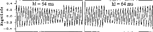
0 . 4 -I
1
1
1
1
02
le 0.2 o
0.0
no
--0.2
--0.4
1
1
1
1
h1=64 ms
li1111i, ,11
11111
|
o = |
120 100 80 60 40 20 0 |
0 20 40 60 40 60 80 100
Time (ms) Time (ms)
Fig. 1. Segments of the acoustic stimuli are presented in the upper panels of each section. The left and right columns show damped and ramped sinusoidal waves, respectively. The half-life of the exponential is 1 ps in the top section, 8 ,us in the middle section, and 64 ps in the bottom section. The carrier frequency is 400 Hz. The repetition period is 50 ,us. The train of current pulses produced by the activated electrode in response to each sound wave is presented in the panel below each sound wave. In these panels, the ordinate (the pulse duration) is in microseconds.
Cochlear Implantees
Fig. 2. Performance of the five cochlear implantees when the half-life is 4 ,us. Stimuli were presented acoustically and went through the speech processor. Two tasks were used to mea- sure discrimination performance. In the first task (unfilled bars), implantees were asked to say if the two sounds were identical or different. In the second task (filled bars), implantees had to choose the interval containing the sound with the more `drum-like' quality. Performance corresponds to the percentage of damped sounds as having the more drum-like quality.
cochlear implantees stimulated directly without the use of the preprocessor (Lorenzi et al., 1997).
In the second experiment, psychometric functions were measured for cochlear implantees BM and DL using procedure B (`more drum-like sound quality' task). The half-life was systematically varied from 1 to 32 ms. The psychometric functions of BM and DL (solid lines with open and filled circles, respectively) are presented in Fig. 3. In both cases, the shortest just-discriminable half-life was between 1 and 1.5 and the longest just-discriminable half-life was between 16 and 24 us. At shorter and longer half-lives, discrimination performance fell off abruptly. For comparison, psychometric functions were measured for three normal-hearing listeners with half-life varying from 0.125 to 128 p. The dotted line with open triangles shows their mean performance. The dashed line without symbols shows the mean of the data obtained by Patterson (1994b) and Irino and Patterson (1996) in similar
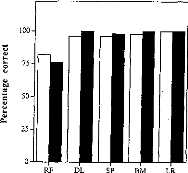
Procedure
In the first experiment, two types of discrimination procedure were used, both of which were 21, 2AFC. In procedure A, listeners were presented a ramped or a damped sinusoid chosen at random in each interval. Thus, there were four possible pairs of sounds: ramped/ramped, damped/ damped, ramped/damped and damped/ramped. They were asked to say if the two sounds were identical or different. In procedure B, they were presented a damped sinusoid in one interval and a ramped sinusoid with the same half-life in the other interval, and asked to choose the interval with the 'more drum-like sound quality'. Thus, performance corresponds to the percentage of damped sinusoids chosen as having the more drum-like quality. Procedure B was also used throughout the second experiment. In the first experiment, the half-life was fixed at 4 ps. In the second experiment, the half-life was fixed within a block and was varied from 1 lus to 32 us from block to block. Each block contained 50 trials in the first experiment and 30 trials in the second experiment.
In both experiments, listeners received visual feedback concerning the accuracy of their response after each trial. Listeners sat in a double-walled soundproof booth, in front of a keyboard connected to the computer controlling the experiment. They received 15 min of preliminary training before participating in each experiment.
Results
The performance of the five cochlear implantees for the first experiment is presented in Fig. 2; the half-life was fixed at 4 its. Each bar is based on 50 trials; unfilled bars for procedure A (`same/different' task) and filled bars for procedure B (`more drum-like sound quality' task). For both tasks, performance was invariably well above chance: the mean performance of the five cochlear implantees was 94.4% (SD 7.12%) for procedure A, and 94.8% (SD 10.54%) for procedure B (p < 0.05 for 61% correct responses). They all heard the difference between damped and ramped sinusoids and chose the damped sinusoid as having a stronger drum-like quality without difficulty. Informal testing with cochlear implantees revealed that the ramped sounds produced the stronger tonal quality, as is the case for normalhearing listeners (Patterson, 1994a, b), and for
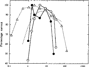
10
100
1000
100 90 80 70 60 50
40
01
Half-life (ms)
Fig. 3. Psychometric functions for cochlear implantees BM (solid lines with open circles) and DL (solid fines with filled circles), showing discrimination performance as a function of half-life. Stimuli were presented acoustically and went through the speech processor. Implantees had to choose the interval containing the sound with the more drum-like' quality. The data from cochlear implantees are plotted along with (1) the mean of the data obtained with three normal-hearing listeners in identical conditions (dotted line with open triangles), and (2) the mean of the data obtained with normal-hearing listeners in similar conditions by Patterson (1994b) and Irino and Patterson (1996) (dashed line without symbols).
conditions.1 For all normal-hearing listeners, discrimination performance was above 90% when the half-life was between 1 ms and 10 ps, but at chance when the half-life was either below 0.125 or above 64 its. In summary, the results of both experiments show that cochlear implantees receiving stimuli through the Digisonic DX10 speech processor can discriminate the timbre of ramped and damped sinusoids as well as normalhearing listeners (when the half-life is 4 its, for instance). However, the results of the second experiment indicate that discrimination is restricted to a narrower range of half-lives in cochlear implantees.
'When the half-life was below 1 ps, the normal-hearing listeners of the present study showed better performance than that reported by Patterson (1994b). This better performance may be due to the fact that Patterson (1994b) did not pro- vide feedback after each response, and he mixed experimental conditions within blocks of trials. It remains, however, unclear why this methodological difference should affect discrimination performance under 1 ps, as opposed to performance over 10 ps.
The average psychometric functions for the cochlear implantees and the normal-hearing listeners who participated in the second experiment are plotted in Fig. 4 (solid Fines with filled circles for cochlear implantees, dotted lines without symbols for normal-hearing listeners). The solid lines with open circles show the mean of the data obtained by Lorenzi et al. (1997) with cochlear implantees stimulated without the intervention of the speech processor. Fig. 4 shows that bypassing the speech processor improves timbre discrimination performance; the effect being stronger at long half-lives than at short half-lives: the longest justdiscriminable half-life is increased by a factor of 25 in the direct stimulation mode. The experiments without the speech processor were performed after those with the speech processor. It is, however, unlikely that practice effects explain the better performance obtained by direct electrical stimulation as the two sets of experiments were separated by a period of 11 months. In addition, all implantees were highly skilled in 21, 2AFC tasks before participating in both experiments.
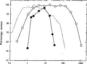
10 100
1000
100 90 80 70 60 50
40
01
half-life (ms)
Fig. 4. Average psychometric functions for the two cochlear implantees stimulated with the intervention of the speech processor (solid fines with filled circles) and the three normal-hearing listeners who participated in the second experiment of this study (dotted fines without symbols). The data are plotted along with the mean of the data obtained by Lorenzi et al. (1997) with cochlear implantees stimulated without the intervention of the speech processor (solid fines with open circles).
The data show that cochlear implantees using the speech processor can consistently label and discriminate the timbre of ramped and damped envelopes, but over a narrower range of half-lives than implantees stimulated directly with the use the speech processor. These data demonstrate that the speech processor of the Digisonic DX10 device degrades the envelope information significantly and affects the timbre of damped and ramped sounds. The loss of fidelity shown in Fig. 1 by the current pulse functions for a half-life of 1 us and 64 us suggests that performance in cochlear implantees is limited by two components of the coding scheme of the Digisonic DX10. At short half-lives (e.g. 1 us), the persistence of the cochlear implant signal and the loss of temporal asymmetry are mainly caused by the long duration of the temporal window (8.2 ils) used for the computation of the 128-point FFT. At long half-lives (e.g. 64 us), the loss of temporal asymmetry appears to be mainly due to the compression circuitry of the device.
Conclusions
This paper describes cochlear implantees' ability
to
discriminate and label the timbre of sinusoids
with asymmetric temporal envelopes. The stimuli were presented acoustically and were transformed by the compressive speech processor of the implant. Stimulation was restricted to a single electrode of the implant.
When the level of the stimuli is adjusted to fit their audibility range, the implantees are as sensitive to temporal asymmetry as normal-hearing listeners, but over a narrower range. In other words, timbre differences elicited by changes in the temporal envelope asymmetry of sounds are less salient in cochlear implantees using their speech processor than in normal-hearing listeners. A comparison between the discrimination performance of cochlear implantees stimulated with and without the use of the pre-processor suggests that the poorer performance of cochlear implantees stimulated acoustically is mainly caused by the 128-point FFI' at short half-lives, and by the compression circuitry of the device at long half-lives.
Temporal asymmetry is a prominent property of speech sounds and sounds produced by musical instruments. It is known to play a role in speech discrimination and timbre perception. For instance, much of the information about the nature of consonants is contained in the 10-40 following an
onset or preceding an offset, and some of the information is in the abruptness of the onset or offset (for a review, see Stevens and House, 1972). Hearing-impaired listeners are therefore likely to make good use of temporal asymmetry when it is available. The present results indicate that it may be important to ensure that cochlear implants (and hearing aids) do not restrict temporal asymmetry unduly when applying compression to control level. Compression is essential for fitting the wide dynamic range of everyday sounds (around 60 dB) into the limited dynamic range available for electrical stimulation (less than 10 dB), and the current results should not be interpreted to suggest that compression should be removed from the speech processors. Rather, the results emphasize the importance of the characteristics of the compression to use, that is, the compression function and the attack and decay times in the case of automatic gain control. In order to preclude the use of spectral cues, the cochlear implants were used in a singlechannel mode during the course of these experiments. This methodological precaution restricts the generality of the current finding. Our results will therefore need to be extended to multi-channel devices before being applied in speech processor design.
Acknowledgements
The first and third authors were at the MRC Applied Psychology Unit (Cambridge, UK) when this research was performed. The first author was supported by a post-doctoral grant from the FYSSEN Fundation. The second author was supported by a CIFRE doctoral grant from
MXM Company. We thank Prof Stuart Gatehouse , Patrick Howell, Catherine Lever and three anonymous reviewers for comments on a previous version of this manuscript.
References
Beliaeff M, Dubus P, Leveau J M, Repetto J C, Vincent P. Sound processing and stimulation coding of DIGISONIC DX10 15-channel cochlear implant. In: Hochmair ES, ed. Advances in Cochlear Implant. 1994; 198-203.
Dobie RA, Dillier N. Some aspects of temporal coding for single-channel electrical stimulation of the cochlea. Hear Res 1985; 18: 41-55.
Handel S. Timbre perception and auditory object identification. In: Moore BCJ, ed. Hearing. New York: Academic Press, 1995; 425-61.
Irino T, Patterson RD. Temporal asymmetry in auditory perception and a 'delta-gamma' theory of asymmetric intensity enhancement in the peripheral auditory system. J Acoust Soc Am 1996; 99: 2316-31.
Lorenzi C, Gallego S, Patterson RD. Discrimination of temporal asymmetry in cochlear implantees. J Acoust Soc Am 1997; 102: 482-85.
Patterson RD. The sound of a sinusoid: Spectral
models. J
Acoust Soc Am 1994a; 96: 1409-18.
Patterson RD. The sound of a sinusoid: Timeinterval models. J Acoust Soc Am 1994b; 96: 1419-28.
Stevens K, House AS. Speech perception. In: Tobias J, ed. Foundations of modem auditory theory. New York: Academic Press, 1972; 1-62.
Conclusion
Lorsque l'on évalue les contraintes psycho-physiques de chaque patient, on s'aperçoit qu'il y a de grandes disparités dans la capacité à coder l'information auditive dans ses trois dimensions le temps, la fréquence et l'amplitude.
Il paraît donc important de connaître les spécificités psycho-physiques de chaque sujet implanté pour adapter au mieux l'interface bio-électrique lors du réglage.
- L'estimation de la fonction de tonie en fonction de l'électrode stimulée nous permet d'attribuer le plus fidèlement possible la répartition fréquentielle.
- L'estimation de la fonction de tonie en fonction de la fréquence de stimulation nous permet d'utiliser la plage de fréquence de stimulation adéquate pour coder le fondamental laryngé.
- L'estimation des fonctions de sonie entre chaque canal nous permet d'adapter l'énergie acoustique à chacune des électrodes.
- La mesure de la résolution temporelle va permettre de régler la fréquence de stimulation moyenne.
La mesure de chacun de ces paramètres peut facilement s'intégrer dans des protocoles rapides lors du réglage, mais ne peut être effectuée que par des sujets implantés adultes et très bien conditionnés. L'élaboration de ces tests psycho-physiques pour une population implantée cochléaire pédiatrique semble être difficile et trop long. La possibilité d'utiliser des méthodes objectives comme l'électrophysiologie pour estimer les contraintes psycho-physiques semble être prometteuse.
L'exploration fonctionnelle des voies auditives fournit une mesure objective de la réponse de ces systèmes à une stimulation électrique. L'utilisation des potentiels évoqués suite à une stimulation électrique de la cochlée (PEAE) semble être intéressante. L'objectif étant d'utiliser ces réponses électrophysiologiques pour des applications cliniques, deux critères importants, la durée et la fiabilité du recueil, doivent être prises en compte. Seules les PEAEP permettent de répondre à ces contraintes ; en effets les PEAE de latences moyennes et tardives ont des durées d'enregistrements longues et des caractéristiques fluctuantes. L'étude des PEAEP des sujets porteurs d'un implant cochléaire est riche en information. Elle permet de mieux comprendre le fonctionnement rétrocochléaire pour des stimulations électriques sur différentes zones de la cochlée à différentes intensités. Elle aurait un intérêt clinique tant au niveau du réglage (en particulier chez l'enfant) qu'au niveau prédictif avant l'implantation. De plus l'utilisation des PEAEP durant l'intervention permettrait de rassurer le chirurgien sur le bon fonctionnement de l'implant cochléaire et du système auditif.
II Les PEAEP
Les potentiels évoqués auditifs précoces (PEAP) enregistrés sur le scalp reflètent le passage des influx nerveux à travers les synapses du système auditif ou le long d'un nerf auditif qui change brusquement d'orientation. Décrits dès 1967 (Sohmer et Feinmesser), ils sont composés de 7 ondes dans un intervalle de temps inférieur à 10 ms (Jewett et Williston, 1971). Chaque onde correspond à l'activité prédominante d'un ou plusieurs générateurs le long du système auditif afférent, de la cochlée au corps genouillé médian (Moore, 1987a, b). L'onde I est générée par les ramifications du nerf auditif le long des cellules ciliées internes. L'onde II est générée par le passage de l'influx nerveux à travers le nerf VIII ainsi que par l'entrée dans le noyau cochléaire. L'onde III est principalement générée par la sortie du noyau cochléaire dorsal (homolatéral) ainsi que par l'entrée dans le complexe olivaire supérieur. Le complexe IV-V serait principalement généré par le colliculus inférieur et le lemnisque latéral (controlatéral). Les ondes VI et VII ne sont présentes que chez 70 % des sujets ; leurs sites générateurs semblent être le corps genouillé médian, néanmoins ils restent mal définis. La caractérisation des PEAP
montre que les latences des ondes sont très sensibles à l'intensité de stimulation et à la zone de cochlée stimulée (Don et Eggermont, 1978 ; Gorga et al, 1988).
Des études chez le singe (Dobie et Kimm, 1980) ont décrit la morphologie des PEAP par stimulation électrique de la cochlée (PEAEP) lors d'une section du nerf facial et/ou vestibulaire. D'autres auteurs (Gyo et Yanagihara, 1980 ; Charlet de Sauvage, 1983) ont comparé les PEAP par stimulation acoustique et électrique (PEAEP) chez le cochon d'Inde ou cobaye. Les latences des ondes en stimulation électrique, sont plus précoces qu'en stimulation acoustique d'environ 1 ms et sont peu sensibles à l'intensité de stimulation. Les mêmes observations ont été faites chez l'humain (Starr et Brackman, 1979). Les variations de latence en fonction de l'intensité dans le cas d'une stimulation acoustique sont donc principalement dues aux processus cochléaires. Le recueil de PEAP par stimulation électrique de la cochlée chez l'humain est donc très riche en informations, car il permet de mieux caractériser et comprendre le système auditif rétro cochléaire en éliminant les distorsions dues à la biomécanique cochléaire.
Le développement de l'implant cochléaire (House et al, 1976 ; Michelson, 1971 ; Simmons, 1966) a grandement facilité la technique de recueil des PEAEP chez l'humain, car on a pu utiliser l'électrode implantée comme stimulateur. Le développement de ces techniques a permis de caractériser les PEAEP en fonction de l'intensité de stimulation chez les sujets porteurs d'un implant cochléaire monoélectrode (Honert et Stypulkowski, 1986). Les résultats suggèrent que les PEAEP sont générés de la même façon que les PEAP, puisqu'il n'existe pas de différence statistique entre les intervalles d11-111, dlll-V et dll-V des stimulations électriques et acoustiques. La comparaison des ondes III et V des PEAP provoquées par une stimulation électrique du noyau cochléaire et des PEAP obtenus par stimulation acoustique chez les mêmes patients confirme ces résultats (Waring, 1992, 1995). Néanmoins les auteurs nous mettent en garde sur les difficultés inhérentes au recueil des PEAEP. En effet la stimulation électrique de la cochlée peut provoquer des réponses myogéniques (Fifer et Novak, 1990 ; Honert et Stypulkowski, 1986), vestibulaires (Honnert et Stypulkowski, 1986) et faciales (Waring, 1992). De plus l'artefact de stimulation est très difficile à extraire du PEAEP. Des études effectuées chez
l'animal (Honnert et Stypulkowski, 1984, 1986) retrouvera les corrélations entre PEAEP et PEAP et
confirment qu'il existe une corrélation entre le nombre de cellules survivantes du ganglion spiral et les amplitudes des PEAEP (Hall, 1990) ; hypothèses qui avaient été faites chez l'humain (Brightwell et ail, 1985 ; Smith et al, 1983).
L'apparition des implants cochléaires multiélectrodes (Clark et al, 1981 ; Eddington, 1980) a rendu possible le recueil de PEAEP en stimulant une partie seulement de la cochlée (Abbas et Brown, 1988). La caractérisation des PEAEP en fonction de l'intensité de stimulation (Abbas et Brown, 1991) n'a pas montré de différences majeures selon les parties de la cochlée stimulées. Néanmoins, il est plus difficile d'obtenir des PEAEP pour des stimulations de la base de la cochlée (Shallop et al, 1993), ce qui contraint les auteurs à stimuler une zone assez grande de la cochlée avec deux électrodes éloignées (Abbas et Brown, 1991) ou d'étudier seulement l'onde V (Miller et al, 1993).
Plusieurs études ont recherché d'éventuelles relations entre les caractéristiques des PEAEP et les capacités perceptives telles que le seuil de détection (Shallop et al, 1991,1993 ; Brown et Abbas, 1994 ; Mason et al, 1994 chez l'homme ; Smith et al, 1994 chez le chat). Malheureusement ces paramètres étaient très peu corrélés et les corrélations ne pouvaient en aucun cas être utilisées en routine clinique à des fins de réglage. D'autres auteurs ont trouvé des relations entre les performances phonétiques des sujets et les caractéristiques des PEAEP (Abbas & Brown, 1991 a,b ; Herman & Thornton, 1992), suggérant que le recueil de PEAEP avant l'implantation, par stimulation électrique du promontoire ou de la fenêtre ronde, pourrait constituer un facteur pronostic.
L'objectif de notre travail a été dans un premier temps de développer une technique fiable de recueil de PEAEP, puis de caractériser ces PEAEP en fonction de l'intensité de stimulation, du site de la cochlée stimulé, de la durée et de la fréquence de la stimulation. Le deuxième temps consistait à comparer les caractéristiques des PEAEP aux mesures subjectives effectuées chez les mêmes sujets afin d'utiliser cette technique de recueil des PEAEP à des fins cliniques.
Ili Recueil et conditionnement des potentiels évoqués auditifs sur implant cochléaire
Si le recueil de potentiels évoqués auditifs
précoces (PEAP) par stimulation acoustique est devenu
quelque
chosed'aisé et de classique, il n'en est pas de même pour les PEAP
par stimulation-électrique
(PEAEP). En effet la grande difficulté du recueil de PEAEP réside dans l'élimination de l'artefact de stimulation qui sature l'amplificateur différentiel d'entrée et masque donc les PEAEP dont l'amplitude est de l'ordre du dixième de microvolt. A titre d'exemple, la stimulation peut aller jusqu'à six volts, ce qui représente un rapport d'amplitude de 6,000,000 entre la stimulation et le recueil. Une étude approfondie sur les paramètres de stimulation et de recueil pour l'obtention de PEAEP de bonne qualité est donc nécessaire.
a/ Le Digistim+®
Pour le recueil des PEAEP, le système spécialisé Digistim+® (cf partie psycho-physique) remplace la partie externe de l'implant cochléaire. Il est alimenté par des batteries, et est commandé par un P.C. via un port série optocouplé. Ce système permet de générer des stimulations dont plusieurs paramètres peuvent varier (électrodes, amplitude, durée de pulse, fréquence de stimulation). Il permet aussi de synchroniser les appareils de recueil de PEA. Ce système permet aussi de stimuler directement la cochlée sans passer par l'implant cochléaire ; il est utilisé pour estimer l'état fonctionnel du système auditif avant l'implantation. Comme nous l'avons décrit plus loin, il est aussi possible de modifier la morphologie de la stimulation en fonction des contraintes dues au recueil de PEAEP (réduction de l'artefact de stimulation sur le recueil).
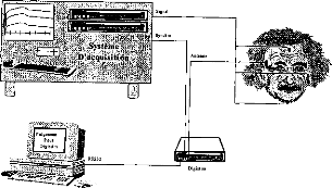
Système
l'acquisition
2
Figure 72 : schéma de câblage du
Digistim+ avec l'appareil de PEAEP lors d'une stimulation
électrique
de la cochlée via l'implant cochléaire
Digisonic ou une électrode temporaire extra-cochléaire
.
13/ L'artefact électrique
L'étude plus approfondie de l'artefact électrique recueilli avec un système d'acquisition de PEAP a deux intérêts :
- L'obtention d'un artefact après stimulation électrique d'une électrode montre qu'il y a une stimulation (Gallego et al, 1997). L'analyse des artefacts sur toutes les électrodes permet donc de vérifier l'intégrité du système. La position des électrodes de recueil adapté à l'acquisition des artefacts de stimulation électrique est à définir.
- Le recueil des potentiels évoqués auditifs électriques précoces, dont l'amplitude est de l'ordre du dixième de micro-volt sur les cinq premières millisecondes, impose d'avoir un artefact électrique peu ample et de courte durée. La position des électrodes de recueil qui réduit au maximum l'artefact de stimulation reste à définir.
Afin de trouver les positions optimales des électrodes de recueil, des mesures in vitro (dans du liquide physiologique) couplées à une modélisation de l'artefact de stimulation ont été effectuées.
Mesure in vitro de l'artefact de stimulation
Nous voulons nous rapprocher au maximum des conditions réelles du recueil des artefacts de stimulation chez un implanté cochléaire. Nous disposons d'une cuve cylindrique de 20 cm de diamètre et 15 cm de hauteur remplie de liquide physiologique, dans lequel on plonge un implant cochléaire Digisonic®. Huit électrodes de recueil sont placées à équidistance sur le périmètre de la cuve dans le liquide physiologique. On place le porte électrode au centre et le récepteur et l'électrode de masse à la périphérie sur l'emplacement d'une des électrodes. L'électrode de masse située au niveau du récepteur récolte les charges accumulées par les condensateurs de couplages des électrodes intracochléaires. Pour la stimulation cochléaire, l'électrode de masse n'a pas d'influence, par contre pour le recueil des artefacts électriques, elle a un effet important car la longueur du dipôle équivalent entre l'électrode de stimulation et l'électrode de masse est environ cent fois plus grande que la longueur du dipôle équivalent entre l'électrode de stimulation et les autres électrodes intra-cochléaires. Le Digistim® nous permet de contrôler la stimulation de l'implant cochléaire (fréquence de stimulation, électrode stimulée, amplitude et durée du pulse) tout en synchronisant le système d'acquisition des artefacts électriques.
A
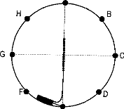
E
Figure 73 : Principe de la
mesure in vitro des artefacts de stimulation mesurés dans un bocal
remplie
de liquide physiologique. Huit électrodes
Afin de minimiser la déformation des traces, on utilise un spectre large pour l'enregistrement (0.2-8000 Hz) et une durée de pulse longue (250 ps). L'électrode testée correspond à celle placée au centre de la cuve (électrode 10).
Plusieurs configurations d'enregistrement par rapport au porte-électrode et à l'électrode de masse de l'implant cochléaire sont testées (28 combinaisons).
|
1000 S., 2000 1000 --0.1 |
6 |
500 -100 --100 --0.1 |
|||||||||||||||
|
0.0 |
0.1 |
0.2 0.3 Temps (ms) |
0.4 |
0.5 |
0 |
0.0 |
0.1 |
0.2 0.3 Temps (ms) |
0.4 |
0.5 |
0.6 |
||||||
Figure 74 : Exemple de recueil de
l'artefact de stimulation avec une tension de E=3.35 volts et
une
durée de pulse de 250ps: V+ =a, V- = c, masse = e (gauche), V+ =
g, V- = c, masse = e (droite)
Les tests effectués n'ont jamais montré une annulation de l'artefact de stimulation. L'amplitude pour une tension d'alimentation de 3.35 volt varie de 1 à 18 mV. Les amplitudes des artefacts sont, les plus faibles lorsque l'électrode de masse est à équidistance des électrodes de recueil (par exemple V+ =c, V- = g, masse = e), les plus élevées lorsqu'une électrode de recueil est proche de l'électrode de masse de l'implant cochléaire (par exemple V+ =d, V- = f, masse = g) .
L'orientation du porte-électrode semble avoir très peu d'effet. Nous avons estimer l'influence de la partie stimulation entre les électrodes intracochléaires en retirant l'électrode de masse du liquide physiologique. Les tests effectués n'ont jamais montré une annulation de l'artefact de stimulation mais l'amplitude pour une tension d'alimentation de 3.35 volt est beaucoup plus faible et varie de 0.1 à 1.5
mV. L'amplitude est la plus faible lorsque les électrodes de recueil (V+V-) sont parallèles ou
perpendiculaires à l'axe du porte-électrode (par exemple V+ = b, V- = d ; V+ = c, V- = g).
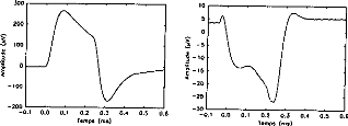
--100
200
--0.1 0.0 0.1 0.2 0.3 0.4 0.5 0 6
Temps
(ms)
300
200
3 100
0.1
0.2 0.3
Temps (ms)
0.4
0.5
06
Figure 75 : Exemple de recueil de l'artefact de
stimulation avec une tension de E=3.35 volts et une
durée de pulse de
250ps: V+ =a, V- = c, (gauche), V+ = g, V- = c (droite)
Le modèle de recueil de potentiel de surface :
Nous sommes partis du modèle de stimulation électrique développé dans l'article 2. Nous avons ajouté l'électrode de masse. Comme l'a montré l'article 2, le fonctionnement en masse-commune de l'implant (toutes les électrodes sont impliquées) localise la stimulation électrique, principalement entre l'électrode de stimulation et les deux électrodes limitrophes. Pour simplifier le recueil de l'artefact électrique, un quadripôle est considéré. Celui-ci est défini par une équation différentielle résoluble par Runge-Kutta sous matlab (en fonction de la durée et de l'amplitude du pulse, et en fonction de l'impédance du milieu physiologique).
V1
·

B
-
·
B'
-------- I ______
C2
v2
------- ------
C2 Cl
C2
R(E)
A
IL
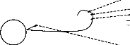
0
Figure 76 : Modélisation de la stimulation par un quadrupôle VA, VB, Vis' Vo. VBA et VBA=V1, VAo=V2
Dans le domaine de Laplace, les équations de VI et V2 sont les suivantes ('p' étant la transformée de Laplace).
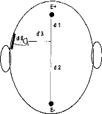
Figure 77 : Orientation et distances des électrodes de recueil par rapport à la stimulation de l'implant.
Pour chaque couple de pôle, le recueil de l'artefact électrique équivalent est fonction de sa distance et de son orientation par rapport aux électrodes de recueils (figure 78). Contrairement aux mesures in vitro, nous faisons ici varier les distance dl et d2.
|
B |
E+ d1 d2 |
|
|
d3 |
||
|
B' |
Figure 78 : Paramètres à prendre en
compte pour le calcul de l'artefact électrique
recueilli sur les
électrodes E+ et E-.
Après quelques simplifications (V+ ) - (V-) peut être considéré comme une combinaison linéaire de V1 et V2 : (V+ ) - (V-)= m.V1 + n.V2
Où lo=0E+, 1'0=0E-, 11=AE+, 12=B'V+, l'2=B'V-, 13=BV+, l'3=BV-. A leur tour chacune de ces
longueurs peut être défini par d1, d2, d3, 0, (p.
Afin de valider le modèle, nous avons comparer les simulations par des expérimentations in vitro.

05

En faisant toutes les combinaisons possibles avec les 8 électrodes de recueil, la position de l'électrode de masse et l'orientation du porte-électrode, l'amplitude varie de 0 à 40 mV. Nous avons trouvé plusieurs configurations où l'artefact de stimulation s'annule. OA doit être perpendiculaire à E+E- et 0 = 0 ou 7c/2 [7c] (figure 78). Les amplitudes maximales sont trouvées lorsque l'électrode de masse est proche d'une électrode de recueil.
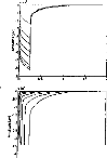
15
0,
Figure 79 : Exemple de recueil de l'artefact de stimulation avec une tension E variable de 2.7 à 5.6 volts et une durée de pulse de 250ps: V+ =c, V- = a, masse = e (gauche), V+ =c, V- = g, masse = e
(droite)
La même étude de simulation sans électrode de masse, trouve des artefacts de stimulation beaucoup plus réduits (inférieurs à lmV).
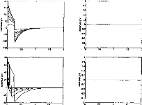
15
08
06
09
02
0:
.08
.08
05
Figure 80 : Exemple de recueil de
l'artefact de stimulation avec une tension E variable de 2.7 à
5.6
volts et une durée de pulse de 250ps: V+ =c, V- = a (gauche), V+
=c, V- = g (droite)
Les résultats obtenus par le modèle concordent avec les mesures in vitro. Nous avons montré que les recueils d'artefact de stimulation sont pour une bonne partie (jusqu'à 95 % de l'amplitude) due au dipôle électrode de stimulation électrode de masse et seulement pour 5% au tripôle B'AB.
Les deux positionnements recherchés sont les suivants :
- pour avoir une amplitude d'artefact de stimulation maximale, il est nécessaire que les électrodes de recueils soit parallèles au dipôle masse / électrode de stimulation. L'amplitude est encore plus importante si une des électrodes de recueil est proche soit de l'électrode de stimulation ou de l'électrode de masse (si dl =d2).
- pour avoir une amplitude d'artefact de stimulation minimale, les électrodes de recueils doivent être perpendiculaires au dipôle masse / électrode de stimulation. L'amplitude est encore plus faible si l'angle = 0 ou 7c/2 [irj et si l'électrode de stimulation est à équidistance des électrodes de recueil.
La durée classique du pulse pour un E de 3.35 volts est généralement comprise entre 5 et 50 ps au lieu de 250ps comme nous l'avons étudié. La morphologie de l'artefact est alors très influencée par les paramètres d'enregistrement du système d'acquisition de PEAP (bande passante du préamplificateur). Les amplitudes de l'impulsion sont, avec un système de recueil classique, divisées environ par 25 (pour 5ps) et 2.5 (pour 50ps) pour une bande passante de 10-8000 Hz. L'amplitude est donc comprise entre 40pV et 800pV pour une durée de pulse de 5ps, et entre 400pV et 8000pV pour une durée de pulse de 50ps.
cl mesure du potentiel de surface (i.e. artefact de stimulation)
Nous avons voulu mesurer les artefacts de stimulation sur le scalp des sujets implantés cochléaires (mesure de potentiel de surface). Après avoir étudier les différents placements possibles des électrodes en fonction des contraintes anatomiques. Deux configurations ont été choisies (figure 81).
- La première position des électrodes de recueil est théoriquement idéale pour la mesure des artefacts électriques des électrodes médianes (les électrodes de recueil sont parallèles au dipôle et l'électrode de masse est proche de l'électrode négative de recueil).
- La deuxième position est théoriquement idéale pour supprimer l'artefact électrique du recueil des électrodes basales (les électrodes de recueil sont perpendiculaires à l'axe formé par l'électrode de stimulation et l'électrode de masse.
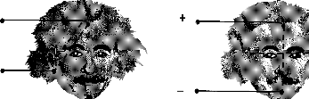
Figure 81
· Meilleur
(gauche) et moins bon (droite) positionnement des électrodes de recueil
pour
l'acquisition de l'artefact de stimulation.
Nous avons testé les artefacts électriques évoqués par une stimulation des 15 électrodes sur 10 patients implantés pour les deux configurations (avec E=3.35 volts, une durée de pulse de 10 ps, et une bande passante du préamplificateur de 0.2-8000 Hz, chaque enregistrement est une moyenne de 100 traces).
15 14 13 18 11 ID g 8 7 8 5 4 3 2 I
800
I 600
o
`g. 100
E
200

`)
140

16 14 13 18 II 10 8 8 7 8 5 4 3 8 I
800
f 400
-`é
200
Figure 82 : Recueil d'artefacts
électriques sur les 15 électrodes (positionnement des
électrodes de
recueil en front - lobule, la durée du pulse est
de 10 ps avec E=3.35 V), chez un sujet porteur d'implant
cochléaire
avec toutes les électrodes actives (gauche), chez un sujet porteur
d'implant cochléaire ayant
une cochlée ossifiée avec
les électrodes 1 et 5 inactives (droite).
La figure 82 représente deux exemples de recueil des artefacts. Chaque pic correspond à une des quinze électrodes. Le patient de gauche a toutes les électrodes fonctionnelles et une cochlée non ossifiée. Le patient de droite a une cochlée ossifiée et deux des quinze électrodes non fonctionnelles. L'ossification de la cochlée modifie la diffusion du courant et l'impédance du milieu, ce qui perturbe l'amplitude et la morphologie de l'artefact.
Pour chaque sujet testé, on a relevé l'amplitude des artefacts correspondant à chaque électrode active. Seules 3 électrodes sur 150 testées n'ont pas évoqué d'artefact électrique (pour le premier positionnement). Dans les 147 autres cas l'amplitude de l'artefact est positive. Par des mesures psycho- physiques, ces 3 électrodes se sont révélées non fonctionnelles.
Par contre 5 électrodes sur les 150 testées n'ont pas évoqué d'artefact électrique pour le deuxième positionnement. Chez 4 sujets sur 10 l'amplitude de l'artefact change de polarité en fonction de l'électrode stimulée (chez deux de ces patients l'électrode 2 ou 3 n'a pas de réponse alors qu'elles sont fonctionnelles). 200
150
100
50
-0
E
< --50
--100
--150
15 14 13 12 11 10 9 8 7 6 5 4 3 2 1
Numéro d'électrode (1:bose 15:opex)
Figure 83 : Exemple d'inversion de polarité sur l'électrode 2 (la durée de pulse est de 10ps, E=3.35 V)
La figure représente les valeurs moyennes (et erreurs standards) des amplitudes des artefacts en fonction de l'électrode stimulée (pour les deux configurations).
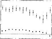
700
600
500
Y. 400
-0 300
200
100
0
--100
15 14 13 12 11 10 9 8 7 6 5 4 3 2 1
Numéro d'électrode (1:base, 15:apex)
Figure 84 : Moyenne et erreurs standards sur 10
sujets porteurs de l'implant cochléaire Digisonice des
amplitudes des
artefacts électriques de chacune des électrodes avec la position
1(
·) et 2 () des
électrodes de recueil (la durée de
pulse est de 10ps avec E=3.35 V).
L'utilisation de la mesure de l'artefact de stimulation pour mesurer l'intégrité du fonctionnement de l'électrode testée est fiable à 100% avec le positionnement 1 des électrodes de recueil. Cela permet, contrairement aux autres systèmes d'implants cochléaires d'utiliser la mesure de l'artefact en routine clinique (Gallégo et al, 1997).
Les amplitudes des artefacts sont en moyenne divisées
par 10 avec la deuxième configuration des
électrodes de
recueil (de 0 à 100 pV). Le modèle ainsi que les mesures in-vitro
sont en accord avec ces
résultats clinique in-vivo. La position Front
- Menton est celle qui est la mieux adaptée au recueil des
PEAEP pour la suppression de l'artefact. La position homolatérale (Front -- Oreille homolatérale) permet d'obtenir des artefacts de grande amplitude.
d/ Les paramètres importants pour le recueil:
o
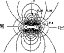
o
Figure 85: Orientation du
champ électrique émis par un dipôle.
Pour les PEAP (en stimulation acoustique) les électrodes de recueil sont positionnées sur le lobule (ou la mastoïde) homolatéral et sur le front (ou le vertex). L'électrode de référence est positionnée généralement sur le lobule contralatéral, mais sa place n'a pas d'influence sur le recueil. Les PEAP reflètent donc l'activité des voix auditives localisées entre les deux électrodes. Le potentiel recueilli est celui du dipôle créé par l'influx nerveux. Son amplitude sera fonction de la distance et de l'angle entre les électrodes de recueil et le dipôle (plus le dipôle sera éloigné, plus l'amplitude sera faible, si l'angle est de 90° le potentiel sera nul). Les PEAP sont donc une combinaison géométrique des différentes activités du système auditif. L'activité correspondant à un dipôle orienté perpendiculairement aux électrodes de recueil ne pourra pas être enregistrée.
Figure 86 : Positionnement
conventionnel des trois électrodes de recueil de PEAP.
La stimulation
acoustique est envoyée à l'oreille homolatérale.
Pour le recueil des PEAP avec une stimulation électrique,
il est difficile d'utiliser un positionnement
conventionnel des
électrodes car le dipôle créé par la stimulation
électrique vient masquer les potentiels
à recueillir. Comme
l'a montré l'étude précédente, ie positionnement
des électrodes de recueil est
déterminant pour la suppression de l'artefact électrique. Pour éviter les phénomènes de saturation de l'amplificateur différentiel d'entrée, il est préconisé d'utiliser un axe de recueil perpendiculaire à l'axe de stimulation. Le problème étant de savoir si cette position idéale pour la stabilité du système d'enregistrement est une orientation qui permet d'obtenir des PEAEP reproductibles, quantifiables, interprétables et d'une morphologie similaire à ceux recueillis par un positionnement homolatéral des électrodes de recueil.
En effet, les potentiels évoqués représentent les champs créés par des dipôles lointains générés par des passages d'influx nerveux. La différence de potentiel (ddp) recueillie est principalement fonction de trois paramètres : la longueur du dipôle, la distance qui sépare le dipôle et les électrodes de recueil, et l'angle entre le dipôle et l'axe des électrodes de recueil. Une mauvaise orientation des électrodes de recueil engendrerait un mauvais recueil de potentiels évoqués.
E+
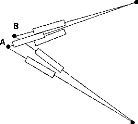
E-
Figure 87 : Principe d'une mesure d'une ddp évoquée par un dipôle éloigné AB dans un milieu Homogène
Certaines études sur les PEAP par stimulation acoustique (Phillips et Thornton, 1995) ont caractérisé les modifications des potentiels en fonction des positions des électrodes de recueil. Il a été montré notamment qu'un enregistrement de PEAP controlatéral était moins exploitable qu'un enregistrement homolatéral, surtout pour l'estimation des seuils. Le recueil homolatéral, permettait entre autre d'obtenir les réponses très périphériques telles que les ondes I et II.
Outre les problèmes liés à l'artefact de stimulation et à l'orientation des électrodes de recueil, le recueil des PEAEP nécessite le moyennage de nombreuses réponses. En effet, l'amplitude des ondes des PEAP ou/et PEAEP dépassent rarement le microvolt alors que la ddp provenant des activités biologiques est de l'ordre de 100 microvolts. Cette ddp provenant des activités biologiques diverses telles que l'EEG, l'ECG, l'EMG est désynchronisée de la réponse auditive. Le moyennage permet de réduire son influence. Son amplitude décroît proportionnellement à la racine carrée du nombre de réponses moyennées ; cette valeur théorique est une sous-estimation des valeurs expérimentales (Grônfors, 1994). L'autre principe permettant d'augmenter le rapport signal sur bruit est de filtrer chaque trace et/ou la trace moyenne de manière analogique et/ou numérique afin de privilégier les fréquences
caractéristiques du PEAP ou/et du PEAEP et de minimiser l'amplitude des fréquences indésirables contenues dans les bruits physiologiques.
La technique de moyennage permet également d'augmenter artificiellement la résolution du convertisseur analogique numérique (CAN) du système de recueil. Avec un CAN de n1 bits qui décompose sa dynamique en 2n1 niveaux, on peut obtenir une décomposition de la même dynamique par (2n2) niveaux en moyennant 2(112-111) signaux. A titre d'exemple, pour passer avec un CAN de 8 bits à une résolution de 18 bits, il suffit de moyenner 1024 fois le signal (pour une sensibilité de 100pV, on passe d'une résolution de 400 nV à 0.4 nV). Ce calcul n'est valable que parce que le signal que l'on moyenne est bruité par un signal non stationnaire.
|
3,75 2,5 1,25 |
|
1 3 4 5 Moyenne
Figure 88 : Moyennage et
résolution
Exemple avec un CAN 2 bits 0-5 V et un signal de 2 V avec
un bruit de 1 V.
La figure 89 représentant l'évolution de la qualité des PEAEP en fonction du moyennage (par pas de 256) et de la position (homolatérale versus controlatérale) des électrodes reflète bien la problématique du choix des paramètres de recueil.
La morphologie des PEAEP en fonction des positions d'électrodes présente des différences en ce qui concerne les premières ondes (ondes II et III). L'enregistrement homolatéral semble demander un moins grand nombre de tracés (512 versus 1024) pour avoir une stabilisation des latences et amplitudes des ondes mais il est beaucoup plus perturbé par l'artefact électrique.
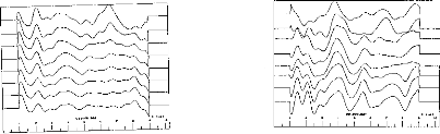
Figure 89 : Exemple de recueil de
PEAEP en homolatéral et contralatérale pour différents
moyennages
(256, 512, 768, 1024, 1280, 1536, 1792, 2048 moyennages).
et Les paramètres importants pour la stimulation:
La qualité des tracés de PEAEP dépend beaucoup des caractéristiques de la stimulation électrique. Morphologie de l'impulsion délivrée par l'implant Digisonic :
L'article 2 modélisant la forme et les caractéristiques de la stimulation électrique générée par l'implant révèle une morphologie asymétrique de l'impulsion comportant une phase positive ample et très courte, puis une phase négative de plus faible amplitude et plus longue durée. Le rapport entre les amplitudes des phases positives et négatives est d'autant plus grand que la durée de stimulation est faible. Comme nous l'ont montré les études psychophysiques sur l'évaluation des seuils de détection et confort, la durée de l'impulsion positive est en moyenne de 30 ps (article 7). Avec cette durée d'impulsion le rapport entre l'amplitude de la phase positive et l'amplitude de la phase négative est d'après le modèle de 10. La partie de la stimulation qui active les neurones du ganglion spiral est donc essentiellement la phase positive, la phase négative ne servant qu'à équilibrer les charges pour éviter les phénomènes d'électrolyse. Des études comparant de la stimulation monopolaire ou bipolaire asymétrique par rapport à la stimulation bipolaire symétrique (Frijns et al, 1996) retrouve ces résultats.
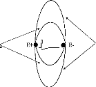
Zone de stimulation
de la phase positive
Zone de stimulation
de la phase négativ
Figure 90 : Zone de stimulation des neurones en fonction de l'asymétrie de l'impulsion
Avec ce type de stimulation électrique, le recueil des PEAEP est quasi impossible car la durée de la phase négative est importante et son amplitude est loin d'être négligeable (entre 200.000 à 600.000 pV pour une durée de 30 ps sur la phase positive), ce qui produit des dérives et des artefacts perturbant le recueil. Comme seule la phase positive est responsable de l'activation des neurones, nous avons modifié la morphologie de la stimulation en inversant l'ordre des deux phases. Commencer par la phase négative permet, comme le montre la figure 91, l'arrêt de la stimulation 50 ps après l'activation de la phase positive tout en maintenant l'équilibre des charges. De plus, d'un point de vu électronique, l'amplificateur différentiel de l'appareil de recueil supporte beaucoup mieux la stimulation ; en effet la phase négative, beaucoup moins agressive, charge négativement l'amplificateur puis la phase positive, très agressive, rééquilibre les charges.
I

Figure 91: Modification de l'impulsion électrique en impulsion triphasique asymétrique Fréquence de stimulation :
Afin d'utiliser le recueil des PEAEP en routine clinique, il est nécessaire de mettre au point des protocoles simples et rapides. Généralement, les fréquences de stimulation sont de l'ordre de 20 Hz. L'obtention d'une courbe moyenne de 2.000 tracés nécessite donc 100 secondes d'enregistrement. Nous savons d'après la littérature et des études préliminaires (Abbas et Brown, 1991 ; Kasper, 1992 ; Gallégo et al, 1997) qu'il est possible d'obtenir des PEAEP à des fréquences élevées tout en préservant la morphologie et les caractéristiques des ondes. Cependant, lorsque la fréquence de stimulation est élevée (100 Hz et plus) les potentiels évoqués de latence moyenne ou tardive se superposent aux enregistrements des PEAEP. Nous avons mis au point une technique de dérive de la fréquence de stimulation qui permet par moyennage d'éliminer sur le recueil les PEA indésirables générés bien après la fenêtre temporelle d'analyse de 5 à 10 ms (figure 92). Il est ainsi possible d'obtenir des PEAEP à des fréquences de stimulation allant jusqu'à 200 Hz soit un temps d'acquisition divisé par 10 par rapport à un enregistrement conventionnel.
|
F (Hz) Variable |
R Na Nb
Figure 92 : Intérêt
de la dérive de la fréquence de Stimulation pour la suppression
des activités
auditives au-delà de la fenêtre temporelle
analysée
Pour des raisons de limitation du système d'enregistrement et non du système de stimulation et/ou de contraintes physiologiques, les études suivantes ont été effectuées avec des fréquences de stimulation de 60 Hz (soit un gain de 3 en temps de stimulation).
fi Faisabilité du recueil de PEAEP via l'implant cochléaire Digisonic
S. Gallégo, C. Micheyl, C. Berger-Vachon, E. Truy, A. Morgon, L. Collet
Acta Otolaryngol (Stockh)
1996, 116, 228-233
L'objectif de cette pré-étude était de mettre au point un protocole d'enregistrement, de stimulation, de traitement et d'analyse des recueils de PEAEP.
Elle a permis de démontrer qu'il était possible d'obtenir des PEAEP de relativement bonne qualité chez plusieurs patients, à différents niveaux d'intensité, sur différentes zones de stimulation de la cochlée. Les ondes II, III et V sont très distinctes,
Elle a mis en évidence les faibles variations des latences des ondes en fonction de la zone et de l'intensité de stimulation. Cela peut s'expliquer, comparer à un PEAP par stimulation acoustique, par le shunt de la biomécanique cochléaire. Seules les amplitudes des ondes ainsi que des mesures de reproductibilité sont dépendantes de la zone et de l'intensité de stimulation.
Acta Otolaryngol (Stockh) 1996; 116: 228-233
Ipsilateral ABR with Cochlear Implant
S. GALLEGO,' C. MICHEYL,' C. BERGER-VACHON,' E. TRUY,2 A. MORGON2 and L. COLLET'
From 'CNRS URA 1447, and 2Department of Otorhinolaryngology, Edouard Herriot Hospital U, Lyon, France
Gallégo S, Micheyl C, Berger-Vachon C, Truy E, Morgon A, Collet L. Ipsilateral ABR with cochlear implant. Acta Otolaryngol (Stockh) 1996; 116: 228-233.
Ipsilateral ABR recording technique was developed with the MXM DIGISONIC DX10 cochlear implant, involving, firstly, setting of recording variables with regard to implant and ABR constraints, and, secondly, enhancement of recording quality by signal processing. The resulting recording quality then enabled us to characterize ABR latency, amplitude and wave reproductibility according to stimulus intensity and stimulation site (electrode stimulated). The findings agree with those of the literature on contralateral human and ipsilateral animal studies. Waves III and V amplitude increased with stimulus intensity. Waves III and V latency was insensitive to stimulus intensity or site. ABR quality diminished basally. Key words: ABR, cochlear implant, electrical stimulation, human, ipsilateral, wave characteristics.
ABR recording
The electrical stimulus used to evoke ABRs was generated using an MXMe DIGISTIM system connected to a PC computer via a serial port. ABR recording was performed using a NICOLET® PATHFINDER II. This system requires the fitting of 3 electrodes (one reference electrode, one anode and one cathode). The PATHFINDER was triggered externally by the DIGISTIM.
The following recording variables were determined after many preliminary trials, using a cochlear implant model and also taking into account electrophysiological constraints: 3 averagings of 256 sweeps; 100 /AT sensitivity; analog bandpass filtering from 0.28,000 Hz; 10 ms analysis time, 512 point window; 50 kHz sampling frequency.
ABR processing
After recording, ABR signals were processed using different processing stages. First of all, the first 400 fis of the ABR signal were excluded so as to eliminate stimulus artefact. Then, the signal was filtered with a digital bandpass of 300-3,000 Hz.
The 3 x 3 intercorrelation matrix was then computed in order to eliminate the most exceptional curves. Finally, the remaining curves were summed and, using an algorithm based on the detection of peaks and infiection points in the signal (5), wave amplitude and latencies were determined. Wave amplitudes were determined on the basis of the length of the wave duration (6).
RESULTS
Characterization of ABRs as a function of stimulation intensity
Fig. 1 shows typical ABR traces recorded from one
electrode
in one patient (SC). The traces were
INTRODUCTION
The recording of ABRs is far more difficult to perform in cochlear implant patients than in non-implanted persons. The amplitude of the electrical stimulation, which is about 10,000,000 times greater than that of the ABR signal, causes saturation of the amplifier. One means of reducing the stimulation artefact consists of contralateral recording: ABRs are recorded in the opposite ear (1). However, another solution could reside in the determination of optimum stimulation variables, which would allow considerable reduction in stimulus amplitude, duration, and leakage across the scalp.
The first aim of the present study was to establish the feasibility of ipsilateral ABR recording; then, once the technique was ready, to elaborate a signal processing technique allowing good-quality ABRs; and finally, to characterize ABRs as a function of 2 variable-stimulation intensity (2) and electrode position (tonotopy) (3).
MATERIAL AND METHODS
Subjects
Three patients implanted with an MXIVI' DIGISONIC DX10 participated in the study. This cochlear implant is a non-conventional auditory prosthesis composed of 15 electrodes (4), the function of which is to replace the peripheral part of the auditory system. These electrodes stimulate the ganglion of Corti and elicit auditory sensations.
X-ray photographe revealed that electrode positioning was roughly the same across patients. Thus, it could be considered that stimulation of a given electrode excited roughly the same frequency region from one patient to another.
General patient characteristics are given in Table I.
(c) 1996 Scandinavian University Press. ISSN 0001-6489
Table I. Patient characteristics
`Performance' is percentage recognition on a Lafon word-list (17 words of 3 phonemes each) by lip-reading plus cochlear implant
|
Deafness |
Implantation |
Performance |
||
|
Patient |
etiology |
duration |
Age |
(LR + CI) |
|
BO |
Accidentai |
6 months |
64 years |
76% |
|
LE |
Evolutionary |
3 months |
60 years |
88% |
|
SC |
Accidentai |
12 months |
44 years |
82% |
recorded at 16 different stimulation levels linearly decreasing from a maximum (80 in arbitrary units determined by the equipment i.e. 0.104 p C/cycle) to 0. The maximum was set just below discomfort level.
Fig. 2 shows the latency and amplitude of waves III and V as a function of stimulation intensity. In each patient, ABRs were recorded for 6 to 9 different electrodes. Because of the large amount of data-- about 50 matrices, as shown in Fig. 2 --findings were clustered by patient. The relationships between stimulation intensity and main ABR characteristics (latency, amplitude and reproducibility) were studied using linear regression. The results of regression analyses (mean, slope, correlation coefficient and signifiance level) are shown in Table II.
In order to compare ABR characteristics between patients, data were then normalized and a regression analysis was performed, the results of which are represented by the scatter plots in Fig. 4a and also given in Table II.
Characterization of ABRs as a function of electrode position (tonotopy)
Fig. 3 shows typical ABR traces obtained from 9 electrodes in one patient (SC). The electrodes were numbered 1-15, basally to apically. Each curve was obtained by averaging about 8,000 traces. Relationships between electrode number and ABR characteristics were studied by means of regression analyses performed on the data clustered by electrode number. As in the previous section, data were then normalized and averaged across patients and regression variables were computed. The obtained relationships are shown in Fig. 4b and the corresponding variables are given in Table II.
DISCUSSION
The results obtained in this study demonstrate
the
possibility of recording ipsilateral ABRs on a coch-
lear implant
(MXM DX10). The good quality of the
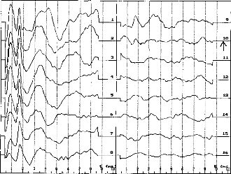
? ? 1 t I 1 1 t I I ? 1 `,"!?
·
14
15
16
Fig. 1. Ipsilateral ABRs from electrode 14 in patient SC for 16 decreasing intensity levels. (The arrow on curve 10 shows patient's subjective threshold).
Table II. ABR variable data according to stimulus intensity and electrode number (position), per patient and average
|
Variable |
Patient |
Mean |
S.D. |
Variation according to intensity |
Variation according to electrode number |
||||||
|
Slope |
n |
R |
p |
Slope |
n |
R |
p |
||||
|
L III (ms) |
BO |
1.90 |
0.0899 |
2.60E-4 |
68 |
0.059 |
NS |
3.85E-3 |
68 |
0.184 |
NS |
|
L III (ms) |
LE |
2.30 |
0.117 |
8.40E-4 |
68 |
0.184 |
NS |
-8.00E-3 |
68 |
0.285 |
<0.02 |
|
L III (ms) |
SC |
1.69 |
0.0905 |
-1.62E-3 |
108 |
0.455 |
<0.001 |
7.30E-4 |
108 |
0.030 |
NS |
|
L III (ms) |
Total |
1.96 |
0.0966 |
-4.90E-4 |
244 |
0.123 |
NS |
-7.40E-4 |
244 |
0.030 |
NS |
|
L V (ms) |
BO |
3.86 |
0.176 |
-1.16E-3 |
68 |
0.133 |
NS |
-0.0231 |
68 |
0.563 |
<0.001 |
|
L V (ms) |
LE |
4.15 |
0.190 |
-1.58E-3 |
68 |
0.206 |
NS |
-0.0130 |
68 |
0.275 |
<0.03 |
|
L V (ms) |
SC |
3.74 |
0.128 |
-9.50E-4 |
108 |
0.190 |
<0.05 |
-5.59E-3 |
108 |
0.162 |
NS |
|
L V (ms) |
Total |
3.91 |
0.161 |
-1.12E-3 |
244 |
0.171 |
<0.01 |
-0.0133 |
244 |
0.329 |
<0.001 |
|
A III (pV) |
BO |
0.362 |
0.152 |
3.89E-3 |
67 |
0.509 |
<0.001 |
0.0150 |
67 |
0.419 |
<0.001 |
|
A III (pV) |
LE |
0.375 |
0.232 |
3.87E-3 |
68 |
0.411 |
<0.001 |
0.0165 |
68 |
0.285 |
<0.02 |
|
A III (pV) |
SC |
0.483 |
0.337 |
6.34E-3 |
106 |
0.475 |
<0.001 |
0.0437 |
106 |
0.484 |
<0.001 |
|
AIII (pV) |
Total |
0.407 |
0.2668 |
4.83E-3 |
241 |
0.440 |
<0.001 |
0.0266 |
241 |
0.394 |
<0.001 |
|
A V (pV) |
BO |
0.312 |
0.149 |
2.49E-3 |
66 |
0.334 |
<0.01 |
0.0117 |
66 |
0.341 |
<0.01 |
|
A V (pV) |
LE |
0.440 |
0.238 |
-3.70E-3 |
68 |
0.385 |
<0.001 |
0.0136 |
68 |
0.229 |
0.060 |
|
A V (pV) |
SC |
0.326 |
0.178 |
-3.38E-3 |
107 |
0.488 |
<0.001 |
0.0202 |
107 |
0.423 |
<0.001 |
|
AV (pV) |
Total |
0.359 |
0.189 |
3.14E-3 |
240 |
0.409 |
<0.001 |
0.0153 |
240 |
0.322 |
<0.001 |
|
COR (%) |
BO |
26.7 |
29.4 |
0.769 |
68 |
0.527 |
<0.001 |
0.954 |
68 |
0.139 |
NS |
|
COR (%) |
LE |
27.6 |
30.0 |
0.802 |
65 |
0.649 |
<0.001 |
-0.521 |
65 |
0.067 |
NS |
|
COR (%) |
SC |
30.9 |
28.6 |
0.399 |
109 |
0.360 |
<0.001 |
2.71 |
109 |
0.355 |
<0.001 |
|
COR (%) |
Total |
28.4 |
29.1 |
0.551 |
242 |
0.464 |
<0.001 |
1.28 |
242 |
0.173 |
0.007 |
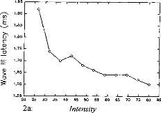
1.60
1.55
20 25
2a:
.30 35 40 45 50 55
Intensity
60 65 70 75 80 135
1.95
.."-^s. 1.90
1.85
m 1.80
· 1.05
E
Q)
Q)
o
4.00 3.95 3.90 3.85 3.80 3.75 3.70 3.65 3.60 3.55 3.50 3.45
3.40
20
25 30 35 40 45 50 55 60 65 70 75 80 B5
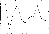
2b: Intensity
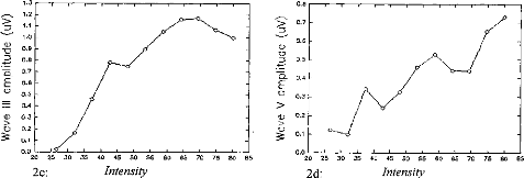
0.8
0.7
D
0.6
0)
M 0.5
0.4
E
0 0.3
Q) 0.2
(1) 0.3
0.1
0.0
25
30 35
45 50 55 60 65
B5
B5
75 80
65 70
60
50 55
40
45
35
30
25
20
80
70 75
Intensity
2d:
1.0
0.9
D 0.8
Cl 0.7
0.6
Cs 0.5
- 0.4
0.2
0.1
0.0
20
2c:
40
Intensity
Fig. 2. Wave III and V latency [(a) and (6), respectively] and amplitude [(c) and (d, respectively] variation according to stimulus intensity in electrode 14 in patient SC (intensity in arbitrary equipment-determined units).
Acta Otolaryngol (Stockh) 116 Ipsilateral ABR with cochlear implant 231
II
V
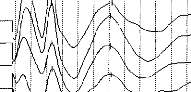
Electrode 14
Electrode 13
Electrode 11
Electrode 10
Electrode 9 Electrode 6 Electrode 5 Electrode 4
Electrode 3
t Cns)IF
Fig. 3. Average ABR from 9 electrodes in patients SC (electrode 3 being the most basal, electrode 14 the most apical).
recordings allowed precise measurement of wave III and V amplitude and latency. Thus, these characteristics were able to be characterized as a function of stimulation intensity and electrode number.
The validity of the present results can be assessed by comparing them to those obtained using acoustic stimulation in normally-hearing patients. Although a direct comparison between wave latencies is impossible, due to the fact that the cochlear filtering stage no longer exists in cochlear implant patients, relative latencies can be compared. The differences between wave III and V latencies obtained in this study (1.95 for patient BO, 1.84 for LE and 2.05 for SC) were within the limits usually obtained using acoustical ABRs in normally-hearing subjects (1.85-2.15 ms (7)). Another correspondence between acoustic and electrical ABRs consisted in the fact that ABRs vanished at a stimulation level corresponding to the behavioral threshold.
The relationships observed in the present study between stimulation level and ABR amplitude and latency are in agreement with the data from previous studies (8, 2, 9). Wave III and V amplitudes increased with stimulation level (the correlation was highly significant).
Wave III and V latencies remained more or less constant for low to moderate intensities and then increased when the stimulation intensity reached threshold (from 0 to 80, about 60 ps for wave III and 195 for wave V). Crosscorrelation increased with stimulation intensity.
The relationships observed between electrode position and ABR amplitude and latency are also in
agreement with the data from previous studies (10,
11, 3). The more apical the site, the greater the amplitude and reproducibility of waves III and V,
and the smaller the latencies (10 ps for wave III latency, 200 ps for wave V latency).
CONCLUSION
The results of the present study are of relevance not
only
to physiologists but also to audiologists regard-
ing objective assessment of auditory performances in
the
cochlear implanted. These results merit further
investigation in a larger number of patients in order
to
obtain a reliable database. There is here a possible
basis for an objective method of threshold setting in children (12).
ACKNOWLEDGMENTS
The authors wish to thank those people and institutions that have supported this study: the MXM company, the Hospices Civils of Lyon, the CNRS, the University of Lyon, the three patients.
REFERENCES
1. Pelizzone M, Kasper A, Montandon P. Electrically evoked responses in cochlear implant patients. Audiology 1989; 28: 230-8.
2. Abbas PJ, Brown CJ. Electrically evoked auditory brainstem response: growth of response with current level. Hear Res 1991; 51: 123-38.
3. Miller CA, Abbas PJ, Brown CJ. Electrically evoked auditory brainstem response to stimulation of different sites in the cochlea. Hear Res 1993; 66: 130-42.
80 60 40 20
-20
-40
- 60
-80
4a:
Intensity
Fig. 4. Variation in wave III and V latency and amplitude and in ABR correlations according to stimulus intensity (a) and electrode number (position) (b).
232 S. Gallego et al.

0.8
0.6
0.4 o o °
00o m0 o o
Its
0.2
0.0
06.
-0.2 8 og c
· ocPo o
L V (P<0.01)
20 40 60 80 100 120 140
Intensity
-0.4
-0.6
-0.8
- 1.0
0
20
40
60 80
100
120
140
0.4 0.3 0.2 0.1 0.0
- 0.1 -0.2
- 0.3 -0.4
Intensity
1.5 1.0 0.5 0.0
- 0.5
0
140
Intensity
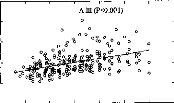
1.5 1.0 0.5 0.0 -0.5
- 1.0 0 20 40 60 80 100 120 140
Intensity
|
- COR (P<0.001) ° 0 o ° e° 008 0 ° 8 S'86'. oo % co 00 e 8 o 1000 o c, §o8 FL 0°0°0°0 ° e0eg°Ir:0° 0 0 ° e ° ° o |
20 40 60 80 100 120 140
Acta Otolaryngol (Stockh) 116

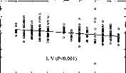
2 4 6 8 10 12 14 16
Electrode number
0.8 0.6 0.4 0.2 0.0
- 0.2 -0.4
- 0.6
- 0.8
-1.0
0
o
0
0
§
o
o 0
o
0
0
0
o
o
8
o
î
ff
g
o
8
0
o
o
L (NS)
0.4
0.3 -
0.2 - 0.1 - 0.0 - -0.1 - -0.2 - -0.3 - -0.4
2 4 6 8 10 12 14 16
Electrode number
1.5
A V (P<0.001)
o
o
Electrode number
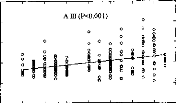
2 4 6 8 10 12 14 16
1.0
0.5
0.0
-0.5
0 2
1.5 1.0 0.5 0.0
- 0.5
- 1.0
4 6
s
0
8 10 12 14 16

Electrode number
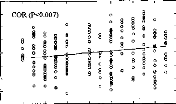
2 4 6 8 10 12 14 16
4b: Electrode number
4. Beliaeff M, Dubus P, Leveau JM, Repetto JC, Vincent P. Sound processing and stimulation coding of DIGISONIC DX10 15-channel cochlear implant. In Hochmair, ed. Advances in cochlear implant. 1994; 198 --203.
5. Boston JR. Automated interpretation of brainstem auditory evoked potentials: a prototype system. IEEE Trans Biomed Eng 1989; 36: 528-32.
6. Gallégo S, Berger-Vachon C, Potier F, Truy E, Collet
L. Automatic diagnosis of electrical BERA using the MXM DX10 cochlear implant. 3rd Paris Int. Congress on Cochlear Implant. Abstracts Book, 1995; 140.
7. Guerit JM. Les potentiels évoqués. Paris: Masson, 1993; 102-16.
8. Abbas PJ, Brown CJ. Electrically evoked auditory brainstem potentials in cochlear implant patients with multi-electrode stimulation. Hear Res 1988; 36: 15362.
9. Allum JHJ, Shallop JK, Hotz M, Pafaltz CR. Characteristics of electrically evoked auditory Brainstem re-
sponses elicited with 22-electrode intracochlear implant. Scand Audiol 1990; 19: 263-7.
10. Kasper A, Pelizzone M, Montandon P. Electrically evoked auditory brainstem responses in cochlear implant patients. ORL 1992; 54: 285-94.
11. Kasper A, Pelizzone M, Montandon P. Intracochlear potential distribution with intracochlear and extracochlear electrical stimulation in humans. Ann Otol Rhinol Laryngol 1991; 100: 812-6.
12. Shallop JK. Objective electrophys from cochlear implant. Ear Hear 1993; 14: 58-63.
Address for correspondence: S. Gallégo
Hôpital Edouard Herriot Pavillon U
URA CNRS 1447
3 Place d'Arsonval
F-69437 Lyon Cedex 03 France
Fax: +33 72 11 05 34.
g/ Le filtrage numérique adapté au PEAEP :
L'utilisation des filtrages numériques post-traitement permettent d'améliorer considérablement les PEAP lors d'une stimulation acoustique (Grônfors, 1994). Dans le cas d'une stimulation électrique, ces filtrages spéciaux ne peuvent pas être utilisés car les artefacts dus à la stimulation électrique viennent détériorer le tracé. Comme le montre la figure 93, certaines fois, il n'est pas nécessaire d'utiliser un post-traitement des tracés. Cela n'est malheureusement pas toujours le cas. Afin d'utiliser les PEAEP pour la clinique et particulièrement pour le réglage de l'implant cochléaire, la qualité des tracés doit être suffisante et stable pour que l'on puisse en extraire les latences et amplitudes des ondes, même celles très précoces.
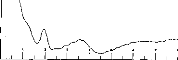
Figure 93 : Exemple de PEAEP sans post-traitement
Pour cela, nous avons développé un traitement des courbes adapté aux contraintes de la stimulation électrique lors du recueil des PEAEP.
S. Gallégo, J Durrant, L. Collet, C Berger
Vachon
Article soumis
L'objectif de cet article est de faire une revue étendue des différents types de traitement numérique des PEAP et d'essayer de comprendre leur principe.
L'article décrit ensuite, à partir de modèles de conduction nerveuse, un nouveau type de filtrage où la fonction de transfert varie avec la latence. En effet, le spectre des PEAEP et / ou PEAP devient de plus en plus grave en fonction de la latence.
Cette nouvelle technique de filtrage tout d'abord simulée sur des modèles de PEAEP bruités puis sur des PEAEP physiologiques a montré une très bonne robustesse vis à vis de différent types de bruits qui viennent se superposer aux tracés:
- Bruit aléatoire ayant un spectre large,
- Bruit électrique correspondant à des artefacts et dérives sur les tracés,
- Bruit biologique spécifique correspondant à des réponses non-auditives dues à la stimulation électrique (vestibule, muscle, nerf facial).
Pour finir l'article montre que les caractéristiques des PEAEP après traitement numérique ne sont pas différentes de celles publiées par d'autres auteurs sans ce type de filtre.
DIGITAL TIME-VARIANT FILTERS ADAPTED FOR RECORDING
OF
ELECTRICALLY AUDITORY BRAINSTEM RESPONSES (E-ABR).
S Gallégol'2, J Durrant1,3, L Collet1,4, C Berger-Vachon1
1- UPRESA 5020 CNRS Laboratory
2- MXM Laboratory
3- University of Pittsburgh
4- ORL dpt, Pav. U, Hôpital E. Herriot
ABSTRACT : The electrically evoked auditory brainstem response (EABR) is useful in objectively measuring the auditory system's response to stimulation via cochlear implant. However, the observed waveform typically is distorted by the electric artifact produced by the implant and other nonauditory signais (i. e. myogenic and vestibular). This paper describes a digital, time-variant filter designed specifically for surface-recorded electrical activity of the hearing system's afferent pathways, specifically under conditions of electrical stimulation. It thus was our objective to improve the quality of EABRs. The transfer function varies along the time continuum, in deference to nuances of neural propagation along a chain of neurons (i.e. the afferent pathway). Simulation showed that this function can extract EABRs in a noisy environment, that is with signal-to-noise ratio (SNRs) of less than -36 dB and facilitate measurement of wave latencies under such noisy conditions. lndeed, we demonstrate detection component wave without significant temporal distortion (i.e. latency shifts) after filtering of noisy EABRs of SNRs down to --24 dB. Such filtering also can reduce substantially both electrical artifact and non-auditory waves of the EABR. Use of this filter under real recording conditions permitted us to measure reliably latencies and interpeak intervals for waves II, III, and V, and observed values compared favourably with data of other authors. We were able to record and measure EABRs even with the most basal electrodes. No significant differences were found according to electrode number.
Key words: EABR, Digital filtering, Signal Noise Ratio
INTRODUCTION
The auditory brainstem response (ABR) (Sohmer and Feinmesser, 1967 ; Jewett and Williston, 1971) is well-known and routine in clinical assessments of the auditory system. It is used to assess quickly the functioning state of the afferent auditory system, namely from the cochlea through the pontine brain-stem pathways. ABR via acoustical stimulation has been known for at least 25 years (Jewett and Williston, 1971). However, interest in electrically-stimulated auditory responses also is long- standing and was fuelled further by the development of the cochlear implant (House et al., 1976; Michelson, 1971; Simmons, 1966; Starr and Brackman, 1979). Use of the EABR to facilitate adjustment of cochlear implant, namely by measurement of the functional status of the auditory system (characterization of EABR I/O functions) and estimation of the threshold level (TL) (measure of apearance of EABR), is of interest. In general, it permits objective measures to be used in cases where subjective responses would be doubtful. However, recording of electrically evoked responses tend to be plagued with electrical stimulus artifact and with responses from nonauditory systems stimulated by the spread of current from the implanted device.
Because the ABR is minute of signal (sub-microvolt range), it is, in general, vulnerable to interference from a variety of signais and/or noise, both physical and physiological. Much work has been dedicated to the processing of acoustically stimulated ABR to minimize the effects of such interference. For example stimulation using alternating polarity clicks helps the suppression of microphonic potentiel and stimulation artifact. Analog filtering following the differential preamplifiers stage of the bioelectric amplifier decreases noise in the recording. Digital filters can improve greatly the signal-to-noise ratio of the ABR (Fridman et al., 1982; Urbach and Pratt, 1986; Pratt et al., 1989; Grônfors et al., 1992,1993) with the advantage of zero phase-shift (Boston and Ainslie,1980). These or comparable approaches to the processing of the EABR, however, have been much less successful.
That interference from electrical stimulus artifact is a considerable problem and is readily appreciated from the fact that it can be over a million-fold greater than the ABR itself. Thus, great care must be taken to avoid saturation of amplifier input and ringing of the analog filter at the preamplification stage. The stimulus artifact also can
last a relatively long time (i.e. up to several milliseconds). Most cochlear implants utilize inductive coupling and the transmission of information from the external device to the implanted package, namely via, a pulse-modulated carrier wave.
Interference from nonauditory signais may arise from several possible sources. Aside from the common source (e.q. electroencephalogram and electrocardiogram), the current may spread to the facial nerve and cause strong interference by myogenic potentiels. There also is the possibility of stimulating the vestibular apparatus and evoking a response from this system.
Techniques used for conventional ABR measurement are less effective with the EABR. The typical analog filtering (100-3000 Hz; -3dB, RC/passive) cannot be used as the artifact actually is prolonged, particularly if the high-frequency cut-off frequency is too low or the low-frequency cut-off frequency is too high. With the EABR, the input analog fiiter ideally should have a wide bandpass (Van den Honert and Stypulkowski, 1986). Digital filtering used for the acoustical ABR also cannot be used, due to the shift in the EABR, namely toward shorter latencies by virtue of the elimination of sound- and hydromechanical-wave propagation and synaptic delays in the auditory periphery. This can cause dramatic distortions, especially during the first milliseconds of the analysis window.
To avert these problems, several techniques can be used. It is possible to put an analog fiiter in the front end of the differential amplifiers (Clarke et al., 1990) to attenuate the electromagnetic interference coming from the transmission of information through the skin, from the external device. If the signal is by-passed during the first milliseconds of a recording (so-called 'blanking') it also is possible to avoid the saturation of the head differential amplifiers. Of course, the waves occurring simuitaneously with the artifact are lost. Techniques based on the subtraction of a model of the artifact, or taking into account the shift have been used (Durrant and Krieger, 1996). However, this signal processing and/or editing can introduce flaws, proportional to the magnitude of the artifact of stimulation. Several cochlear implants also allow the stimulation pulse to be biphasic in order to decrease the influence of the artifact on the recording. Nevertheless, the success of EABR recording still is strongly affected by the capabilities of the recording amplifier (not equal among
systems/manufacturers). The techniques just described are by no means optimal, and not all of these techniques are possible via available ABR test systems and/or within the expertise of the examiner.
There thus has been little work to establish signal processing methods specifically for the EABR. The technique described herein was developed in consideration of the properties of the EABR and was tested both by simulation and in actual implanted subjects. Although the clinical application of interest here is the post-implant evaluation via EABR measurement, it also is conceivable to use this technique for pre-operative testing in the implant candidate, i.e. via promontory stimulation using a transtympanic electrode. This technique also should be adapted ultimately to the study of electrically evoked middle- and long- latency auditory evoked potentials and to the EABR obtained with a brainstem implant.
MATERIAL AND METHODS COCHLEAR IMPLANT
The cochlear implant employed in this study was the DIGISONIC, a 15-electrode transcutaneous device (Beliaeff et al., 1994). It is manufactured by the firm MXM (Antibes, France). It is composed of two distinct parts; an external and an internai component (figure 1). The external device performs an acoustical signal analysis leading to the extraction of relevant speech information. This information is passed to the internai (implanted) device. The signal processing is based on the Fast Fourier Transformer. The external device computes, in real time, the spectrum of the acoustical signal for 64 bands of 122 Hz in the range of 0 to 7.8 kHz. The acoustical signal is sampled at 15.6 kHz. The analysis window is 128 points. Frequency bands are grouped before being distributed to the electrodes. The transcutaneous interface is composed of two antennas, one emitting and the other receiving. Generally, active electrodes are located from 5 to 20 mm from the base. The internai part performs the decoding of the information received by the internai antenna and stimulates the programmed electrodes.
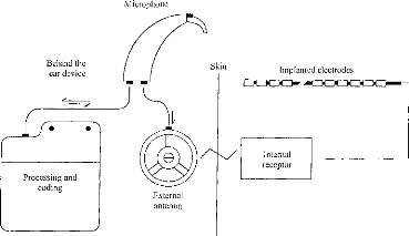
Bellind the ear device
Skin
Implanted electrodes
Microphone
EICDIC{},-
Internai
receptor
Processing and
coding
External
antenna
Figure 1: Block diagram of the DX10 DIGISONIC cochlear implant. Information is transmitted from the speech processor to the internai part on a carrier, wave using amplitude modulation. The carrier frequency was 4 MHz.
Stimulation was accomplished via the Common Ground mode, wherein the addressed electrode is activated and ail the others are connected to ground. The stimulus is produced by a pulse generator; the pulse is of a constant amplitude, but variable in length. As illustrated in figure 2, the equivalent circuit of each electrode/channel of stimulation is a series capacitor and resistor, fed by the pulse generator. The stimulus delivered is biphasic and asymmetric. Adjustment of the series capacitor permits very precise equalization of the positive and negative charges transferred which, in turn, is extremely important for preservation of physiologie integrity of the tissues. The pulse duration ranges from 5 to 310 ps. The pulse generator can source 3 mA over a 2 kohm load. For recording EABRs, the external package is replaced by a specialized device manufactured by MXM, the DIGISTIM. The DIGISTIM is battery-powered and controiled by a persona! computer through an opto-isolated serial port. This system allows the generation of a pulse with several adjustable parameters, i.e. choice of electrode, magnitude, pulse duration, and stimulation frequency. Synchronization of the evoked potential test system is made possible by an external trigger pulse produced by DIGISTIM.
r
|
C=150 nF |
||||||||||||||
|
R=1 kohm |
||||||||||||||
Figure 2: Simplified description of the DIGISONIC cochlear implant stimulation in the labyrinth. Impedance can be represented by a pure resistance (about 2 kohm in vivo). Mean amplitude is zero volt. Positive and negative parts of the pulse are not symmetrical but charges are equal. Phase-Iocking of the fibers occurs mostly on the positive part.
ANALYSIS OF THE EABR--THEORETICAL BACKGROUND: THE ABR AND HEARING SYSTEM
The ABR represents electrical fields sampled on the scalp. These fields are produced by sources remote to the electrodes; the recorded signais thus are characterized as being far-field potentials. They are the consequence of nerve-impulse propagation along the auditory pathways from the inner ear to the inferior colliculus at the upper margin of the pontine portion of the brain stem (for review, see Durrant and Lovrinic, 1995 and Durrant and Wolf, 1991). The stimulation of choice for these characteristically short-latency potentials (i.e. with principle waves falling within 10 ms.) is a brief transient, such as the acoustic click, which excites a relatively wide population of nerve fibers (due to spectral splatter) with excellent synchronisation (due to temporal precision of the stimulus). The ABR primarily reflects, therefore, afferent activity of auditory nerve fibers in the Vllith nerve and the brainstem (Moore, 1987b). Each wave cornes from a virtual source which can be represented as a dipole with an amplitude and an angle (phase and space) (Williston et al., 1981; Pratt et al., 1983; Scherg and Cramon, 1985). Consequently, a given pair of recording electrodes, that is sampling between any two points on the head, registers an overall waveform that is the resultant of the combined phasor and vector summation of the overlapping time-series of compound potentials excited at the various levels of the
peripheral and brain-stem auditory pathways. Waveform morphology thus is influenced not only by stimulus spectral and temporal characteristics, but also orientation of the recording `dipole' with respect to those of constituent sources dipoles.
Clinical methods of recording employ disc electrodes (e.g. silver or gold) with an electrolyte paste affixed to the skin. At moderate intense stimulus levels, the typical ABR appears as a series of 5-7 waves occuring within a time frame of 10 milliseconds. The EABR, however, typically shows only three waves in a 6ms time interval (waves II, III & V, in reference to the acoustically evoked response) (Van den Honert and Stypulkowski, 1986; Abbas and Brown, 1988; Shallop et al., 1990). Nevertheless, the generation of EABRs waves is fundamentally the same as for the ABR, but with the input stage of the system (the organ of Corti) being effectively`bypassed (Van den Honert and Stypulkowski, 1986; Waring, 1995). This eliminates the initial propagation and synaptic delays, moving the ensemble earlier into the measurement time window. Wave I, from distal Vlllth nerve usually is obscured by the stimulus artifact, regardless of method of analysis. Wave II derives from the transition between the VIllth nerve and the passing into the brainstem (WIler et al., 1988). Wave III is generated when the nervous signal leaves the cochlear nucleus. The IV-V complex originates somewhere along the contrelateral lemniscus to the controlateral inferior colliculus (Moore, 1987b; Millier and Jannetta, 1982; Legatt et al., 1988; and Durrant et al., 1994).
co co
Figure 3: Aspect of the compound nerve impulse related to the distance from the stimulation.
Most of the afferent auditory nerve fibers (90% or more) are
myelinated (Spoêndlin and Schrott, 1988, 1989; Moore, 1987a,b). The fiber
diameter is characterized by a
normal distribution centred between 2 and
44.im .(Spoëndlin and Schrott, 1988, 1989),
as is conduction velocity. Furthermore, the farther from the origin of stimulation, the Iess synchronous are the neural potentials. Consequently, the density of discharge of the fibers also is typically represented by a normal distribution which becomes increasingly broader the farther the potentials are sampled from the source. Namely, the width increases Iinearly with the distance (Figure 3). Normative studies of the ABR support this theory (John et al., 1982). This fact however, is somewhat obscured in the ABR waveform, because of the diverse origins of wave I to V (Zapala et al., 1992), further complicated by temporal dispersion due to the frequency-place encoding performed by the cochlea (Don and Eggermont, 1978; Gorga et al., 1988). This resuits in the superposition of wave components, depending upon stimulus intensity (Zapala et al., 1992). Electrical stimulation, however, simplifies matters in that the responses originate from essentially the same region of the VIllth nerve (i.e., again, cochlear propagation delays are eliminated).
RECORDING PARAMETERS
The Pathfinder II (Nicolet Biomedical) was used to record the EABRs. The ipsilateral montage commonly employed clinically for recording the ABR was used here: the noninverting input of the preamplifier was connected to a gold-cup electrode at hairline, at midiine, and the inverting input was connected to an electrode placed on the ipsilateral earlobe. The ground electrode was affixed to the contralateral earlobe. The recording parameters employed, however, were slightly different of those used in ABR protocol. Full-scale sensitivity was +/-50pV. A wide bandpass (0.2 Hz-8000 Hz) was used. The sampling rate (50kHz) was well above the highest frequency of interest in the EABR; such oversampling is desirable in order to minimize the influence of noise (Grônfors and Juhola, 1995). Each response recording derived from an average of 512 stimulus repetitions. This is a relatively low N by clinicat standards, but it should be born in mind that the subjects were under general anesthesia. Consequently, time was of the essence, but some sources of noise (i.e. myogenic from movement) were naturally reduced. A test and two retests of EABR were performed for each stimulus condition for purposes of determining reproducibility of the responses.
Stimulation, again was delivered by the Digistim, triggering the Pathfinder II. In our study, for each patient, we tested from 4 to 9 electrodes equally spaced along the array from base to apex. For each electrode, we have recorded a threshold among 16 intensity levels, along a linear scale from comfort level (CL) to 0. The duration of the pulse was chosen a the parameter by which to vary intensity. For each condition, we made three recording. The stimulus rate was 60 Hz, chosen to be above the line frequency used in Europe (50Hz). (This clearly would not be an appropriate choice in countries like the United States and Canada where the line frequency is 60 Hz.). This frequency admittedly is to high for ABRs elicited by acoustic stimulation (i.e. due adaptation), yet it not poses problems, in our experience, with electrical stimulation. This is because adaptation for electrical stimulation is more dependent upon refractory period than pure adaptation (Brown et al., 1990 ; Abbas and Brown, 1991 b). After acquisition, the data were transferred to a personal computer for further processing, where upon the filter algorithm was implemented and the filter function applied. Consequently, the choice of system for data acquisition is not critical to the analysis procedure.
FILTER TECHNIQUE
Considering the neuroanatomical and neurophysiological bases of the ABR, the width of the component waves are expected to increase with latency, which in fact occurs overall. Consequently, each wave has not only a characteristic latency, but also a characteristic spectrum. Wave I then is expected to be more easily detected using a high frequency filter; the opposite is expected for wave V, since, for longerlatency waves, the spectrum is more robust in the lower frequencies. However, the filters previously described for ABR/EABR have fixed transfer functions. The choice of bandpass is made according the ABR/EABR's average spectrum. In more recent studies, on the other hand, Pratt (1989) and Gronfors (1993) have described digital filters adapted to each wave, i.e. by latency.
The filter involved a transfer function designed according to certain nuances of neural conduction. As shown in Fig. 3, the compound action potentials which develop along a neural pathway are products of the conduction velocity and axonal length. If the spectra of such signais are measured , there is observed a band-pals whose center
frequency follows approximately a hyperbolic function. For proprietary reasons (re future product development), the details of the filter function cannot be divulged. Nevertheless, certain important characteristics can be described.
The conduction velocity depends upon diameter of the nerve fiber; as the diameters follow a Gaussian distribution (Spoendlin, 1988, 1989), the waveforms perhaps can be modelled by a Gaussian pulse whose width influences the latency function. The formula approximating the wave can be written as follows:
Onde(t)= A. exp( (t--t0)2)
Where tO corresponds to a latency for which the response is at the maximum, b is the time constant of the wave, and A is the wave's amplitude at t=t0.
As the form of the wave presumably follows a naturel law, the convolution of the wave by a Gaussian pulse of the same half-life duration centered on zero will maximize the peak of a wave. The distribution of the theoretical wave is calculated, starting from work in this laboratory and values in the literature (Gallego et al., 1996, 1997; Abbas and Brown, 1988).
exp(--( t, )2)
S(t) = E(t)*
fexp(--(b,)2.dx)
Where b is the time constant of the theoretical wave and E(t) is the waveform centered on the point where one wishes to detect a peak.
The filter that we have developed was inspired by the formula above, however, it takes into account only a part of the total EABR wave, corresponding to essentially 95 % of the energy of the theoretical wave (t = [ -1.96-2b, 1.96+2b]).
This filter is designed with the goal of maximizing the peaks of the EABR waves and trying to protect the integrity of the EABR while eliminating those waves not belonging to the EABR proper. We thus endeavour to eliminate all waves that do not correspond to the desired ones, that is to say, those that do not fall within plus-or-
minus three standard déviations. To- conctruct the theoretic EABR, we -have based it
on the wave III. In effect, this wave, contrary to wave II and IV-V complex, is well isolated from the others. There thus is no overlapping of wave III by the others, so it can easily be dissociated from EABR (fig. 5a). The duration of wave III also is the most stable. Utilizing a conventional digital filter (filter pass band of 150-3000 Hz (Gallégo et al., 1996)), we have measured the width of wave III in a sample of 10 implanted subjects with the Digisonic. The width of wave III is 1.05 ms with a standard deviation of 0.138 and a peak latency of 2.06 ms with a standard deviation of 0.186.1f one considers that this width corresponds to approximately 95 % of the energy of the wave (this would be +/- 2b'), one thus can measure the time constant of wave III (b' = 1.05/4 = 0.26 ms). We, therefore, have filtered the signal in the manner that only waves falling within plus-or-minus three standard deviations ( for t=2.06 ms. b' = [0.16,0.37]). We have made the assumption that at the instant of t=0, the neural influx evoked by electric stimulus was perfectly synchronized. We then varied b' linearly as function of the latency such that at t=2.06, b'=0.25 and b' varies linearly as a function of t.
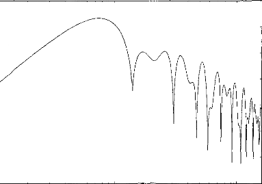
20
10
0
m
--10
20
30
40
50
100 1000 10000
Frequency (Hz)
Figure 4 : Transfer function of the numeric filter when the latency is 2,06 ms and b=0,288 ms.
The ideal formula for the filter is:
t )2)
exp(--( , t )2)
exP( (b' (t)+3.sd(t))
(b (t)-3.sd(t) E(t)*
E(t)*
exp(--( , )2 .dx)
exp( ( )2 .dx)
(b (t)+3.sd(t))
(b (t)-3.sd(t))
where b'(t)=a.t
exp(--( )2)
E(t)* (b (t)-3.sd(t)
f exp(--( , 2.dx)
x = --2(b' (t)+3sd(t)) (b (t) -- 3 .sd(t))
2(b' (t) + 3sd(t))
The formula utilized experimentally is only an approximate of
the theoretical one. The
analysis window is from 4 b'(t) to infinity, so the
equation becomes:
* porte(2(b'(t)+ 3.sd(t)))
* porte(2(b'(t)+ 3.sd(t)))
exp(--( t )2)
(b (t)+3.sd(t))
-- E(t)*
2
2(b' (t)+3sd(t))
f exp(--( ) .dx)
x = --2(h' (t)+3sd(t)) (b (t)+3.sd(t))
Where b' +1- 3 sd(t) takes the values following the function of latency: for t=0.5 ms b'(t)-3sd(t)=0.04 ms, b'(t)-3sd(t)=0.10 ms ; t=1 ms b'(t)-3sd(t)=0.08 ms, bi(t)- 3sd(t)=0.20 ms ; t=2 ms b'(t)-3sd(t)=0.16 ms, b'(t)-3sd(t)=0.40 ms....
Figure 4 shows the filter transfer function for a 2.06-ms-latency component. ( This filter function is simulated for 1024 points, ranging from 100 Hz to 15 kHz on a logarithmic scale.) This function can be represented by a bandpass filter with a peak at 750 Hz. The shape of the filter's frequency response is maintained for components of other latencies. There is a slight linear shift with latency: the peak is at 3kHz for t=0.51ms, at 1.5kHz for t=1.03ms, at 750Hz for t=2.06ms, at 375 Hz for t=4.12ms
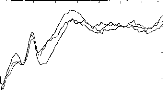
The EABRs were sampled over a 10.24 ms window to yield a time-ensemble of 512 data points. However, only the data points representing latencies from 0.5 to 8 ms were considered in the calculation of the filtered response. Like Durrant and Krieger (1996), we found some truncation of the initial part of recording to be essential. On the other hand, experience simply dictates that period beyond 8ms is of no value in assessing EABRs.
After having filtered the three tracings from the same intensity of stimulation, we calculated a mean. To facilitate visualization of the response, we then blanked the first 0.5 ms of the trace to eliminate (or minimize) stimulus artifact. To permit objective determination of the presence or absence EABRs, we calculated a 3x3 matrix of cross-correlations among the three traces (note above). The window studied extends from 1 to 7 ms (300 data points). The EABR was considered to be presence when the cross correlation was greater or equal to 0.15 for two out of three traces (Pearson correlation : p=0.01).
0.5 0.0 --0.5 --1.0
RESULTS
2 3 4 5 6 7 8
--1.5
0
Fig 5a.
0.6 0.4 0.2 0.0 --0.2 --0.4
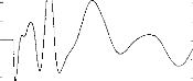
|
2 |
3 |
4 |
5 |
7 |
a |
Fig
Figure 5: EABRs before (5a) and after (5b) digital processing. After filtering the three curves, the intercorrelation function leads to a time shift equal to -20ps between the first and the second averages (Pearson coefficient=0,85), -60ps between the second and the third averages (Pearson coefficient=0,93), 20ps between the first and the third averages (Pearson coefficient=0,91). The detection of the waves indicates LII=1,22ms, LIII=1,98ms, LV=3,74ms, A1l=0,52pV, Al11=0,99pV, AV=0,57pV. (It also is possible to demonstrate wave IV, but focus upon waves II, III, and V as they were the most robust in our recording).
Figure 5 shows a EABR before and after using the digital filter. Latencies of the waves are not affected. With a simple peak-finding subroutine, latencies and amplitudes of the waves can be easily measured. The short-latency components are well separated from the stimulus artifact.
Latency of wave II (ms) Latency of wave III (ms) Latency of wave V (ms) wave H-III interval (ms) wave III-V interval (ms)
means and s.d
|
means and s.d Van den Honert & |
means and s.d Abbas & Brown, 1988 |
Means and s.d. Kasper et al., 1992 |
|
|
1.28 (0.17) |
1.20 (0.14) |
1.36 (0.19) |
1.38 (0.09) |
|
NS |
NS |
NS |
|
|
2.05 (0.18) |
2.10 (0.15) |
1.99 (0.23) |
2.16 (0.18) |
|
NS |
NS |
NS |
|
|
3.86 (0.28) |
4.09 (0.26) |
3.99 (0.37) |
3.94 (0.22) |
|
*** |
NS |
NS |
|
|
0.77 (0.06) |
0.95 (0.16) |
0.63 (?) |
0.75 (?) |
|
*** |
? |
? |
|
|
1.81 (0.14) |
1.83 (0.17) |
2.00 (?) |
1.79 (0.17) |
|
NS |
? |
NS |
Table I: Average EABR latencies ( 11 subjects, for 58 tested electrodes) compared to values observed in other studies (Van den Honert and Stypulkowski, 1986 ; Abbas et Brown, 1988 ; Kasper et al., 1992). A comparison of the mean values has been performed using a comparison of mean values statistical test (NS: no significant difference ; ***: significant difference, less than 0,05 ; ?:no tested).
The robustness of the noise reduction of this filter function also was assessed. A model EABR was constructed based upon results of other researchers (table I, right part) and from our own laboratory (Gallégo et al., 1996, 1997) and imbedded in white noise for several signal-to-noise ratios (SNRs). The model EABR comprised component waves having latencies of 1.28ms, 2.06ms and 3.86ms respectively. Corresponding widths are 0.71ms, 1.15ms, and 2.15ms.
Figure 6 shows the effect of the addition to the model EABR a white noise before and after digital filtering (the SNR was varied between +18 to --24 dB in steps of 6 dB). Despite the addition of noise, it is notable that wave II, III and V always can be identified. There latencies are very stable.
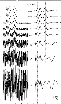
t
i
r
S/N (da)
+6
--6
..-
--12
--18
--24
2 ms
--
Figure 6: Resistance to noise of the filter function. A white noise has been added to the signal (EABRs + white noise) ; signal is represented before (left) and after (right) this signal processing. The signal-to-noise ratio varied from +18 to --24 dB in steps of 6 dB.
Figure 7 compares the evolution of the cross-correlation, between the original mode! EABR and that buried in noise, with and without digital filtering (with SNR varied between +18 and --48 dB in 6 dB steps). Each point corresponds to an average of 100 repetitions. (Also indicated are the standard errors). Without digital filtering, we could detect the EABR only down to SNRs of --24 dB. With digital filtering, we could detect the EABR down to --36 dB SNR. For noisier waveform, there no longer was a significant correlation between the noisy signal and the original signal.
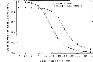
O Signal + Noise
· Signal + Noise filtered
N
Figure 7: Cross-correlation between a model EABR and model EABR buried in noise (white noise added, bandwidth of 25,000 Hz) as a function of the signal-to-noise ratio. Each point corresponds to a mean of 100 repetitions (mean and standard errors) before (open circles) and after filtering (close circles). The dashed lines (for R = 0.15) demark the limit of validity of the measurement of EABR (p=0.01).
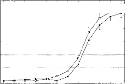
o Signal + Noise
· Signal + Noise filtered
300

250
rn
200
C.)
C
o
150
Q)
TD 100
ô 50
E)
18 12 6 0 --6 --12 --18 --24 --30 --36 --42 --48
Signal Noise ratio (dB)
Figure 8: Mean of absolute latency shifts (intercorrelation) between a model EABR and model EABR buried in noise (white noise added, bandwidth of 25,000 Hz) as a function of the signal-to-noise ratio. Each point corresponds to a mean of 100 repetitions (mean and standard errors) before (open circles) and after filtering (close circles). The dashed lines (for t = 50-100 ps) demark the limit of validity latency of the EABR (from 2.5 to 5 data points). Below this zone we consider that there is no significant displacement between the two curves. Above this zone, the model EABR in noise with and without filtering are two different.
Figure 8 compares the variations of the maxima of inter-correlation between the noisy EABR-(filtered or not) and the original EABR. This gives an idea of the changes in latency of the waves due to the addition of the noise. Each point corresponds to an absolute value of the average of 100 repetitions. (Also indicated are the standard errors.). The latency shifts are contained within +0.5 ms (with an mean value of 0.25 ms representing chance). The latency shifts can be considered negligible for mean values from 50 to 100 ps (2.5 to 5 data points). The digital filter does not cause latency shifts for SNRs down to --24 dB. For
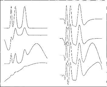
Figure 9: Demonstration of suppression of interfering signais (myogenic, vestibular, etc.). Input signais, i.e. EABR + interference (Ieft-hand panel) are auto-scaled to full-scale, dictated in some case by the magnitude of the interfering signal. Filtered, output signais (right-hand panel) are plotted on the same scale.
Another test of the filter transfer function was to evaluate
its ability to suppress waves
where the spectrum is incompatible in their
latency with waves evoked by auditory
stimulation. It was noted above that
such waves could derive from myogenic,
vestibular, or other sources. Figure 9 shows several model non-EABR waves. It can be seen in figure 7 that such waves are strongly attenuated.
In this work, EABRs have been recorded and filtered for 11 implantees, for several electrodes (a total of 58), and with different stimulation levels for each electrode (16 levels). For each recording we first determined if there was presence or absence of an EABR (again, cross-correlation of >= 0.15). Then, for the traces which were recognized as EABRs we measured the latencies and interpeak intervals of waves III, and V. We then averaged the values by electrodes, then by across patients. Table I indicates the latencies and interwave latencies for waves II, III, and V measured on 11 subjects. These average values have been compared with results given other authors on others cochlear implant system (Van den Honert and Stypulkowski, 1986; Abbas and Brown, 1988; Kasper et al., 1992 respectively tested on single channel 3M, multi-channel Nucleus and lnaired, multi-channel Inaired systems). Most of the comparisons are not significantly different (10 out of 12). Results obtained after filtering match the usual values given in the literature. EABRs were recorded even when the perception was that the stimulus was very faint.
DISCUSSION
EABR quality was found to be improved substantially by the use of a time-variant filter function adapted to the auditory system. Each wave undergoes filtering that is latency-specific and can be easily extracted from the overall EABR and background noise. No latency shift is introduced by the processing. Noise and signais commonly interfering with the EABR were reduced dramatically by this filter function, both in stimulations and actual recordings. Consequently, the myogenic wave typically occurring at about 6.0 ms (Fifer and Novak,1990) and the putative vestibular wave occurring at 0.5 ms (Van den Honert and Stypulkowski, 1986) were effectively suppressed. Indeed, most of the problems seen with EABRS are reduced by this filter function; including suppression of the de shift induced by the stimulus artifact. Furthermore, wave II which was not systematically seen in other studies (Van den Honert and Stypulkowski,1986) is always extracted.
Latencies of waves II, III, and V measured using the filtered responses were found to compare favourably with the values reported by other workers with other cochlear implant systems (Van den Honert and Stypulkowski, 1986; Abbas and Brown,1988; Kasper et aI.,1992). This agreement suggests our method to be valid and to yield accurate Iatency measures. The potential to record responses in all cases and with stimulation by all electrodes is particularly significant for intraoperative and clinical applications of EABR analysis. Altogether, 58 electrodes were tested in 11 patients. We thus did not have the sorts of failures reported by others (e.g. Van den Honert and Stypulkowski, 1986; Abbas and Brown, 1991).
Finaily, the time-variant filter function proved to be very robust in coping with noise added to model EABRs. The model EABRs were reliably recorded in broad-band noise to SNRs below -36 dB. Furthermore, this filter does not cause latency shifts for SNRs <= -24 dB. Consequently, EABRs can be recorded using low-level stimulation, as indeed was demonstrated by actual EABR recordings. Such performance is particularly important in working with paediatric patients in the clinical setting, wherein time is of the essence. Using this filter should substantially reduce the analysis time by reducing the number of stimulus repetitions needed for each average, thereby permitting the exploration of more electrodes.
ACKNOWLEDGEMENTS
The authors acknowledge those individuals and institutions who made this work possible: the MXM company, the Hospices Civils of Lyon, the Centre Nationale de Recherche Scientifique, the Université Claude Bernard, professors Eric Truy and Alain Morgon, and certainly the eleven implantees.
REFERENCES:
Abbas PJ, Brown CJ, Electrically evoked brainstem potentials in cochlear implant patients with multi-electrode stimulation, Hear. Res. vol.36, pp.153-162, 1988.
Abbas PJ, Brown CJ, Electrically evoked auditory brainstem response: Growth of the response with current level, Hear. Res. vol.51, pp.123-37, 1991a.
Abbas PJ, Brown CJ, Electrically evoked auditory
brainstem response: refractory properties
and strength-duration functions,
Hear. Res. voI51, pp.139-48, 1-991-13-.
Beliaeff M, Dubus P, Leveau J-M, Repetto J-C, Vincent P, Sound Signal Processing and Stimulation Coding of the DIGISONIC DX10 15-Channel Cochlear Implant, advances in Cochlear Implant Ed Hochmair-Desoyer IJ & Hochmair ES, pp.198-203, 1994.
Boston JR, Ainslie PJ, Effects of analogue and digital filtering on brainstem auditory evoked potentials, Electroenceph. Clin. Neurophysiol. vol.48, pp.361-364, 1980.
Brown CJ, Abbas PJ, Gantz B, Electrically evoked whole-nerve action potentials: parametric
data from human cochlear implant users, J. Acoust. Soc. Am. vol. 88, pp.2205-2210, 1990. Clarke CJA, Thomson DR, Gibson WPR, Measurement of auditory brainstem responses evoked
by electrical stimulation with a cochlear implant, Brit. J. Audiol. vol.24, pp.145-149, 1990.
Don M., Eggermont J.J., Analyses of click-evoked brainstem potentials in man using high-pass noise masking, J. Acoust. Soc. Am., vo1.63(4), pp.1084-1098, 1978.
Durrant J, Krieger D, Artifact reduction in evoked potential recording via polynomial curve fitting--feasibility study, Abstracts of the Nineteenth Midwinter Research Meeting of the Association for Research in Otolaryngology, pp.77, 1996.
Durrant J.D., Lovrinic J.H., Bases of Hearing science, 3rd ed. Williams & Wilkins, Baltimore, 1995.
Durrant J.D., Martin W.H., Hirsch B., Schwegler J., 3CLT ABR analyses in a human subject with
unilateral extirpation of the inferior colliculus, Hear.Res., vol.72, pp.99-107, 1994.
Durrant J.D., and Wolf K.E., Auditory evoked potentials: basic aspect. In Hearing Assessment, 2nd Ed., W.F. Rintelmann, ed. Pro-Ed: Austin, pp.321-381, 1991.
Fifer RC, Novak MA, Myogenic Influences on the Electrical Auditory Brainstem Response (EABR) in Humans, Laryngoscope, vol.100, pp.1180-1184, 1990.
Fridman J, John ER, Bergelson M, Kaiser JB, Baird HW, Application of filtering and automatic peak detection to brain stem auditory evoked potentials, Electroenceph. Clin. Neurophysiol., vol.53, pp.405-416, 1982.
Gallégo S, Micheyl C, Berger-Vachon C, Truy E, Morgon A, Collet L, Ipsilateral ABR with cochlear implant, Acta Otolaryngol.(Stockh), vol.116, pp.1604-1610, 1996.
Gallégo S, Truy E, Morgon A, Collet L. EABRs and surface potentials with a transcutaneous multielectrode cochlear implant. Acta Otolaryngol (Stockh), vol 117, pp.164-168, 1997.
Gorga MP, Kaminski JR, Beauchaine KA, Jesteadt W. Auditory brainstem responses to tone burst in normally hearing subjects, J. Speech. Hear. Res., vol.31, pp.87-97, 1988.
Grônfors T, Juhola M, Johansson R, Evaluation of some non recursive digital filters for signais of auditory evoked responses, Biol. Cybern., vo1.66, pp.533-536, 1992.
Grônfors T, Peak identification of auditory brainstem responses with multifilters and attributed
automaton, Computer Methods and Programs in Biomed., vol.40, pp.83-87, 1993.
Grônfors T, Juhola M, Effect of sampling frequencies and averaging resolution on medical
parameters of auditory brainstem responses, Comput.
Biol. Med., vol.25(5), pp.447-454, 1995.
House WF, Berliner K, Crary W,
Graham M, Luckey R, Norton N, Setters W, Tobin H, Urban J,
Wexler M, Cochlear implants, Ann. Otol. Rhinol. Laryngol., vol.85(suppl 27), pp.1-93, 1976.
Jewett DL, Williston JS, Auditory evoked far-fields averaged from the scalp of humans, Brain, vol.94, pp.681-696, 1971.
John ER, Baird H, Fridman J, Bergelson M, Normative values for brain stem auditory evoked potentials obtained by digital filtering and automatic peak detection, Electroenceph. Clin. Neurophysiol., vol.54, pp.153-160, 1982.
Kasper A, Pelizzone M, Montandon P, Electrically Evoked Auditory Brainstem Responses in Cochlear Implant Patients, O.R.L., vol.54, pp.285-294, 1992.
Legatt A.D., Arezzo J.C., and Vaughan H.G., The anatomic and physiologic bases of brain stem auditory evoked potentials, Neuroligic. Clinics., vol.6, pp.681-704, 1988.
Michelson RP, Electrical stimulation of human cochlear: A preliminary report, Arch. Otolaryngol., vol.93(3), pp.317, 1971.
MOler A.R., and Jannetta P.J., Evoked potentials from the inferior colliculus in man, Electroenceph. Clin. Neurophysiol., vol.53, pp.612-620, 1982.
Miller A.R., Jannetta P.J., Sekhar L.N., Contributions from the auditory nerve to the brainstem auditory evoked potentials (BAEPs): Results of intracranial recording in man, Electroenceph. Clin. Neurophysiol., vol.71, pp.198-221, 1988.
Moore JK, The human auditory brain stem: A comparative view, Hear. Res., vol.29, pp.1-32, 1987a.
Moore JK, The human auditory brain stem as a generator of auditory evoked potentials, Hear. Res., vol.29, pp.33-43, 1987b.
Pratt H., Har'el Z, and Golos E., Geometrical analysis of human three-channel Lissajous' trajectory of auditory brain-stem evoked potentials, Electroenceph. Clin. Neurophysiol., vol.56, pp.682-688, 1983.
Pratt H, Auditory Brainstem Evoked Potentials Peak Identification by Finite Impulse Response Digital Filters, Audiology, vol.28,pp.272-283, 1989.
Scherg M., von Cramon D., A new interpretation of the generators of BAEP wave I-V; Results of spatio-temporal dipole model, Electroenceph. Clin. Neurophysiol., vol.62, pp.290-299, 1985. Shallop JK, Beiter AL, Goin DW, Mischke RE, Electrically Evoked Auditory Brain Stem Responses (EABR) and Middle Latency Responses (EMLR) Obtained from Patients with the Nucleus Miltichannel Cochlear Implant, Ear Hear., vol.11(1), pp.1-15, 1990.
Simmons FB, Electrical stimulation of the auditory nerve in man, Arch. Otolaryngol., vol.84, pp.2-54, 1966.
Sohmer H, Feinmesser M, Cochlear action potentials recorded from the external ear in man, Ann. Otol. Rhinol. Laryngol., vol.76, pp.427-435, 1967.
Spoendlin H, Schrott A, The Spiral Ganglion and the Innervation of the Human Organ of Corti, Acta Otolaryngol.(Stockh), vol.105, pp.403-410, 1988.
Spoendlin H, Schrott A, Analysis of the human auditory nerve, Hear. Res., vol.43, pp.25-38, 1989.
Starr A, Brackman DE, Brainstem potentials evoked by electrical stimulation of the cochlea in human subjectes, Ann. Otol. Rhinol. Laryngol., vol.88, pp.550-560, 1979.
Urbach D, Pratt H, Application of finite impulse response digital filters to auditory brain-stem
evoked potentials, Electroenceph. Clin. Neurophysiol., vol.64, pp.269-273, 1986.
Van den Honert, Stypulkowski PH, Characterization of the electrically evoked auditory
brainstem response (ABR) in cats and humans, Hear Res , vol.21, pp.109-126, 1986.
Waring MD, Auditory brain-stem responses by electrical stimulation of the cochlear nucleus in
human subjects, Electroenceph. clin. Neurophysiol., vol.96, pp. 338-347, 1995.
Williston J.S., Jewett D.L., and Martin W.H., Planar curve analysis of the three-channel auditory
brainstem response: a preliminary report, Brain. Res., vol.223, pp.181-184, 1981.
Zapala DA, Gould HJ, Mendel MI, Place specific influence on the wave I to V interpeak latency
of the auditory brain-stem response, J. Acoust. Soc. Am., vol.92(6), pp.3174-3184, 1992.
L'utilisation du filtrage numérique permet d'obtenir des PEAEP d'une qualité suffisante et stable intra- et inter- session pour un patient donné ; cela permet d'étudier les paramètres qui influent sur les caractéristiques des PEAEP afin de les utiliser si cela est possible en routine clinique pour des tests pré- per- et post implantation.
al Adaptation et PEAEP
Il est important avant toute chose de quantifier l'effet de la durée et de la fréquence de stimulation sur les caractéristiques des PEAEP. Ces deux paramètres représentant deux formes d'adaptation du système auditif suite à une stimulation électrique pourraient détériorer la qualité des tracés de PEAEP. La caractérisation de ces deux phénomènes permettrait d'élaborer des protocoles d'enregistrement qui minimiserait ces effets.
Durée de stimulation et PEAEP :
Lors d'une stimulation acoustique continue, l'activité neurale du système auditif décroît puis se stabilise à un certain niveau (Kiang et al, 1965). D'après la littérature, cet effet serait essentiellement produit au niveau de la cochlée lors de la transduction de l'énergie acoustique en influx nerveux électrique (Edgermont, 1985). Lors d'une stimulation électrique de la cochlée, les avis sur les modifications des réponses en fonction du temps de stimulation sont partagés. Malgré l'absence de la transduction, certains auteurs montrent de grosses modifications de l'activité (Brimacombe et al, 1984 ; Dynes et al, 1992) en fonction de la durée de stimulation ; d'autres auteurs par contre ne trouve pas de variations des réponses (Killian et al, 1994). Ces divergences pourraient provenir de l'état fonctionnel du système auditif des populations étudiées par ces différents articles. Les populations animales qui sont rendues sourdes depuis longtemps et que l'on vient de réactiver par stimulation électrique de la cochlée présenteraient lors des premiers jours de stimulations des phénomènes d'adaptation importante ; à contrario des populations animales que l'on rendrait sourdes subitement puis que l'on stimulerait électriquement ne présenteraient pas de phénomènes d'adaptation de l'activité en fonction du temps de stimulation.
Aucune étude chez l'homme n'a été effectuée pour évaluer cet effet d'adaptation neurale par stimulation électrique de la cochlée. Lorsque l'on veut recueillir des PEAEP il est néanmoins nécessaire de pouvoir estimer ce phénomène car une adaptation importante provoquerait une disparition progressive des PEAEP en fonction du temps de stimulation.
Six sujets implantés cochléaires depuis plus de 1 an ont participé à cette étude. Pour chacun d'eux l'électrode 4 (basale) et 14 (apicale) ont été testées à 70% de la dynamique.
|
timulation 1 |
Stimulation 10 |
Somme |
|
1-50 |
1-50 |
E |
|
151-200 |
151-200 |
E |
|
301-350 |
301-350 |
|
|
451-500 |
451-500 |
E |
|
1151-1200 ----- |
1151-1200 |
E |
|
Stop 3 min |
Stop 3 min |
Le protocole d'enregistrement schématisé figure 94 consiste à recueillir dix séries de 12 traces de 50 stimulations espacées de 100 stimulations. Après chaque série, un temps de repos de 3 min est nécessaire pour revenir à un état dit normal de l'excitabilité du système auditif. Ainsi chacune des 12 traces représente respectivement les PEAEP générés à 0-1, 3-4, 6-7, 9-10, 12-13, 15-16, 18-19, 21-22, 24-25, 27-28, 30-31, 33-34 secondes. Comme la fréquence de stimulation est de 50 Hz, chaque traçe représente respectivement les PEAEP générés par les 0-50, 150-200, 300-350, 450-500, 600-650, 750800, 900-950, 1050-1100, 1200-1250, 1350-1400, 1500-1550, 1550-1600ème stimulation. Afin d'améliorer le rapport signal sur bruit de chaque tracé, une sommation des dix séries est effectuée. Au final chaque courbe correspond à un moyennage de 500 stimulations. Afin d'analyser les PEAEP, le filtrage numérique post-traite
Figure 94 : Protocole d'enregistrement des PEAEP pour la mesure de l'adaptation.
Comme l'exemple du patient #1 représenté figure 95, la qualité des PEAEP pour chaque trace de 500 passages est bonne. Des mesures de latence et amplitude des ondes II, III, V ainsi que la mesure d'énergie globale du tracé ont été effectuées. L'analyse statistique par anova n'a pas montré de différence de latences ou/et amplitude ou/et énergie en fonction du temps de stimulation, cela pour les 2 électrodes testées.
Cette étude démontre que pour la population testée (stimulation électrique de la cochlée depuis plus d'un an), le phénomène d'adaptation de l'activité du système auditif en fonction de la durée de stimulation est négligeable à 70 % de la dynamique (pour les électrodes basales comme apicales) pour l'obtention des PEAEP. Il n'y a ni baisse ni désynchronisation de l'activité en fonction du temps de stimulation. Dans ce cas de figure le protocole d'enregistrement des PEAEP peut être indépendant du temps de stimulation ; seuls des facteurs augmentant le rapport signal sur bruit et temps d'enregistrement peuvent être pris en compte.
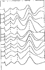
0 0 0.5 1.0 1.5 2.0 2.5 3:0 3.5 4.0 4'.5 5.0 5.5 6.0
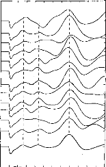
0 0 0.5 1.0 1.5 2.0 2.5 3.0 3.5 4.0 4.5 5.0 5.5 6 0
Figure 95 Exemple de PEAEP pour
le Patient # 1 en fonction du temps de stimulation pour
les
électrodes 14 et 4. La dernière trace correspond à
la moyenne des 12 :
Par contre, cette étude limitée au niveau des conditions étudiées ne répond pas à l'éventuelle adaptation de l'activité auditive pour des populations sourdes que l'on vient juste de réhabiliter (cas des PEAEP pré et per opératoire). De plus l'adaptation à des niveaux faibles d'intensité n'a pas été étudiée.
Période réfractaire et PEAEP :
Des études effectuées chez l'animal (Stypulkowski et van den Honert, 1984 ; Miller et al, 1993) puis chez l'homme (Abbas et Brown, 1991 ; Kasper, 1992) ont décrit la possibilité de mesurer la période réfractaire des circuits du système auditif avec les PEAP et/ou PEAEP et potentiels d'actions composites. Cette période réfractaire se traduit par une diminution de l'activité et de la synchronisation en fonction de la fréquence de stimulation acoustique et/ou électrique de la cochlée.
Les études de Abbas et Brown 1991 ont décrit les modifications de l'activité qui génère les PEAEP en fonction de la durée inter-stimulation électrique de la cochlée au niveau des amplitudes de l'onde V. Par contre aucune étude n'a analysé les latences et amplitudes des ondes II, III et V afin de mieux localiser et comprendre cette période réfractaire suite à une stimulation électrique.
L'objectif est d'étudier les modifications des caractéristiques des PEAEP en fonction de la durée inter- stimulation afin d'évaluer la fréquence de stimulation critique pour l'obtention des PEAEP.
12 sujets implantés cochléaires ont participé à cette étude. L'électrode 14 (apicale) a été testée à 70% de la dynamique pour des durées inter-stimulation de 17, 5, 4, 3, 2.5, 2, 1.6 et 1.3 ms.
Comme le montre le protocole d'enregistrement schématisé figure 96 les enregistrements se font en deux temps. Tout d'abord les PEAEP sont recueillis avec un délai inter-stimulation fixe de 17 ms (A). Puis on recueille les PEAEP avec deux stimulations espacées de dT et 2T-dT (B) ; cela permet d'avoir en moyenne le même nombre de stimulations par seconde que dans le premier enregistrement. De manière numérique, on soustrait ensuite le PEAEP (B) au PEAEP (A) ; la réponse obtenue représente le PEAEP provoqué par la deuxième impulsion.
A
B
B-A
Figure 96 : Principe de la mesure de période réfractaire via les PEAEP
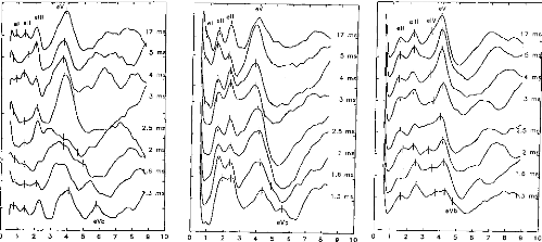
2 3 4 5 6 7 8 9 10
17 ms 5 ms 4 ms
3 ms
2.5 ms 2 ms 1.6 ms
Tg
eVb
2 3 4 5 6 7 8 9 10
0 1 2 3 4 5 6 7 8 9 10
0
Figure 96 : Exemple sur 3 sujets des PEAEP en fonction de la durée inter-stimulation
Comme le montre la figure 97, la morphologie des PEAEP reste stable jusqu'à des durées inter stimulation de 1.3 à 4 ms suivant le patient. En dessous de cette durée, on assiste à une décomposition de l'onde V en 2 ondes Va et Vb. Cette décomposition pourrait s'expliquer par le fait que l'onde V réflète l'activité de plusieurs générateurs dont un qui a une période réfractaire plus longue que les autres. Ces variations inter-sujets semblent être intéressantes à analyser et à prendre en compte lors du réglage.
Malgré la tendance figure 98, les variations des amplitudes des ondes II, III ne sont pas statistiquement différentes suivant la durée inter-stimulation (F=1.5 ; F=1.3). Par contre l'amplitude de l'onde V subit de grosses modifications (F=3.4 p<0.005) ; cela peut sûrement s'expliquer par la décomposition de l'onde V qui réduit les amplitudes.
Lorsque l'on regarde l'évolution des latences des ondes, on montre une augmentation statistique des latences lorsque l'on réduit la durée inter-stimulation. Lorsque l'on compare les fluctuations des latences en fonction de la durée inter-stimulation, on constate d'après un test statistique que ces variations sont principalement générées avant l'onde II (F=8.359, p<0.001) ; les intervalles II-III, III-Va et II-Va ne sont pas dépendants de la durée inter stimulation.
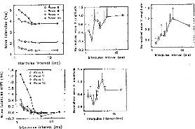
|
e:; Wave II |
|||
|
5 |
e, |
rl |
Wave III |
|
E 4 î% 3 |
0 |
Wave V |
|
10
1
Interpoles intervol (ms)
= 0.8
0.6
0
· 1.5
E
· 1.2
n 0.9
0.4
15 0.2 1
10
Interpulse intervol (ms)
1.5
E 1.2
e
F 0.6
2
1.4
E 1.2
1.0
15. 0.8 0.6 0.4
.2 0.2
· 0.0
e --0.2
Figure 98 : Latences et amplitudes en fonction de la durée inter-stimulation chez 12 sujets.
La mesure de la période réfractaire de chacun des étages du système auditif le long du tronc cérébral peut être couplé à une mesure de la résolution temporelle de chaque patient. L'estimation de manière objective de la résolution temporelle d'un sujet implanté permettrait estimer le nombre d'informations par seconde que peut traiter le patient afin d'adapter le traitement du signal, en particulier la fréquence moyenne de stimulation.
En conclusion de ce paragraphe, l'adaptation liée au temps de stimulation a apparemment peu d'effet sur les PEAEP ; l'adaptation liée à la période réfractaire débute à des durées inter stimulation de 3 à 4 ms en moyenne. Ces deux constatations nous permettent d'élaborer un cahier des charges très peu contraignant pour l'obtention des PEAEP.
13/ Effet de l'Intensité de stimulation et de la zone stimulée
Nous avons voulu caractériser les modifications des caractéristiques des PEAEP (latences, amplitudes des ondes II, III et V) en fonction des caractéristiques essentielles de la stimulation via l'implant cochléaire multiélectrode Digisonic.
S. Gallégo, J Durrant, E. Truy, C Berger Vachon, L.
Collet
Article soumis
Dans un premier temps, l'article décrit un protocole qui permet d'étudier les PEAEP en fonction de l'intensité et du site de stimulation électrique de la cochlée. Après avoir démontré l'intérêt de l'utilisation de la durée de l'impulsion pour coder l'intensité, l'article montre qu'il est possible d'obtenir des PEAEP sur tous les sujets testés et que les caractéristiques des ondes (II, III et V) sont similaires à celles obtenues avec d'autres types d'implants cochléaires.
L'étude statistique montre que l'amplitude des ondes croit avec l'intensité de stimulation (codée par la durée de l'impulsion) et croit lorsque l'on se dirige vers des stimulations apicales.
Par contre les latences sont des paramètres peu dépendants de l'intensité de stimulation (en durée de l'impulsion).
La latence de l'onde V (et l'intervalle III-V) varie en fonction du site de stimulation. Elle décroît légèrement lorsque l'on se dirige vers des stimulations apicales.
L'estimation par les PEAEP des fonctions de sonies des sujets implantés et en particulier des seuils de détection et de confort est un sujet intéressant pour l'aide au réglage de l'implant.
EFFECT OF STIMULATION INTENSITY AND INTRACOCHLEAR SITE
ON
ELECTRIC AUDITORY BRAINSTEM RESPONSES IN HUMAN USING A
MULTICHANNEL
COCHLEAR IMPLANT WITH A VARIABLE DURATION PULSE.
S Gallégo (1,2), JD Durrant (1,3), E Truy (4), C Berger-Vachon (1), L Collet (1,4).
1- UPRESA 5020 CNRS Laboratory
2- MXM Laboratory
3-Departments of Communication Science and Disorders and Otolaryngology, Pittsburgh
4- ORL Dept, Ed. Herriot Hospital
ABSTRACT : The Electrical Auditory Brainstem Response (EABR) elicited via a cochlear implant is an interesting tool for analysis of retrocochlear mechanisms, i.e. the impontine brainstem. In this paper, EABRs were studied with respect to stimulation intensity and the excited part of the cochlea. The parameter used to control the stimulus intensity was the pulse duration. Latencies were found to be rather stable, which was not seen in all previously reported studies (namely variations of waves III and V). This tact can be explained by the shape of the stimulating pulse. By judicious choice of the stimulus waveform, synchronization of the fibers is enhanced by making it more difficult for firing on the negative phase of the pulse. Amplitudes of waves II, III, and V were slightly increased with the stimulation intensity. EABR latencies and intentais (mostly wave V and III-V interval) decreased from base to apex. This might reflect a compensatory mechanism to the propagation delay from the base to apex in a normal cochlea. The amplitudes of wave II, III, and V also were increased from base to apex; this may be linked to cells'density along the cochlea which progressively increases from the base to the end of the first cochlear turn.
Key words: Cochlear implant, EABR, characterization, pulse duration, level effect, site effect.
INTRODUCTION
Auditory Brainstem Responses (ABRs) recorded, on the surface of the scalp, presumably reflect (primarily) the propagation of nerve action potentials through the lower auditory pathway, involving multiple synaptic delays, decussation(s) of fibers, and discontinuities of the volume conductor. First described in the literature in 1967 (Sohmer and Feinmesser, 1967), the ABR comprises up to 7 waves with in a time window of approximately 10 milliseconds (Jewett and Williston, 1971). Each wave cornes from the activity of one or more generators distributed along the afferent auditory system, from the cochlea to the middle geniculate body (Moore, 1987a,b). The electrically elicited ABR has met with increased interest. The Electric Auditory Brainstem Response (EABR) has been studied in animais and humans alike and compared systematically to acoustically evoked ABRs (e.q. see Gyo and Yanagihara, 1980 and Starr and Brackman, 1979, respectively). Wave latency has been found to vary little with stimulus intensity, unlike the acoustic ABR. The acoustically elicited response is well-known to demonstrate a pronounced latency-intensity function which, in turn, is considered to reflect the influence of cochlear propagation (Don and Eggermont, 1978, 1993, 1994, Gorga et al, 1988). In any event, the place encoding mechanism precludes scrutiny of place-specific stimulation without the influence of wave-propagation-based latency effects. The EABR potentially allows the characterization of the activation of the auditory system without such `distortion'.
The development of cochlear implant (House et al, 1976; Michelson, 1971; Simmons, 1966) opened the door to the study of the human EABR since the implanted electrode can be used as a stimulator (Starr and Brackman, 1979). Van den Honert and Stypulkowski, 1986 characterized the effects of the stimulus intensity in patients fitted with a single-channel cochlear implant. Results showed that EABRs are generated in a similar manner to acoustical ABR with no significant difference found for the interpeak intervals 11411, III-V, II-V. Recent comparisons between acoustically and electrically evoked ABR - in the same patients with brainstem implant (stimulation at the level of the cochlear nucleus) confirms this result for wave III, and V (Waring, 1992, 1995). Nevertheless, authors emphasize the technical difficulties of recording the EABR. First, electrical stimulation can introduce myogenic and facial nerve responses (Fifer and Novak, 1990; Van den Honert and Stypulkowski, 1986;
Waring, 1992). Furthermore, the stimulation artifact itself is very difficult to remove from EABR recordings. Nevertheless, studies performed in animais (Van den Honert and Stypulkowski, 1984, 1986) have shown correlations between EABR and ABR recordings and revealed the relation between the number of surviving cells in the spiral ganglion and EABR magnitude (Hall, 1990), as had been assumed in the human (Brightwell et al, 1985; Smith and Simmons, 1983).
The arrivai of a new generation of cochlear implants (Clark et al, 1981; Eddington, 1980) made possible EABR recordings utilizing place-specific stimulation (Abbas and Brown, 1988), albeit constrained by the spread of electrical excitation due to the transmission-cable-like electroanatomy of the cochlea. Results, however, were not remarkably different when different parts of the cochlea were stimulated (Abbas and Brown, 1991a). In any event, it proved difficult to reliably record EABR for basal stimulation of the cochlea (Shallop et al, 1993), and it appeared that wide intervals on the cochlea were being stimulated (Abbas and Brown, 1991a) or for recording problem (locking of the fibers and signal to noise ratio) to study only wave V and not waves II and III (Miller et al, 1993).
In these studies, the pulse amplitude was adjusted to modify the stimulation intensity. Consequently, when the intensity of electrical current was raised, the portion of the cochlea stimulated also was increased, i.e. via the spread of excitation. It is a wellestablished property of neurons in general (see Colombo and Parkins, 1987, for review and model) that stimulus duration also can used to increase the stimulation intensity. This has also be demonstrated specifically for auditory neurons (Pfingt et al, 1991). The inherent advantage of manipulating stimulus pulse duration, versus intensity, is that the length of the stimulated interval on the cochlea can be held constant. The use of the pulse duration to modify the stimulus intensity allows better phase locking of the auditory nerve fibers, at least when stimulus intensity is kept low. In the case, the shorter the duration of the pulse is, the better the synchronization becomes. Poor locking of the fibers in very low loudness, when constant duration pulse are used, can explain the poor correlations seen between the perceptual threshold and EABR appearance in human cochlear implantees (Shallop et al, 1991; Mason et aI, 1994; Brown et al, 1994) and in the cat (Smith et aI, 1994).
The purpose of this report is to characterize in detail the EABR obtained in such subjects with short pulse duration, generally below 100 ps, according to stimulus intensity (i.e. duration, with amplitude held constant) and the putative cochlear segment excited. This method of stimulation (i.e. short duration with amplitude constant) enhances EABR recording (measure of waves II, III and V) by better synchronization.
MATERIAL & METHODS Subjects
Eleven implantes, fitted with the DIGISONIC cochlear implant (CI), participated in this study (8 males and 3 females, aged from 3.5 to 69 years).
The French DIGISONIC MXM cochlear implant
The DX10 DIGISONIC (Beliaeff et al, 1994, Chouard et al, 1995, Gallégo et al, 1997c) is a 15-channel, transcutaneous, cochlear implant device made by the French firm, MXM (06, Vallauris). It comprises an external and an internai part. The external part incorporates the emitting antenna which is juxtaposed the internai receiving antenna (i.e. forming the transcutaneous link between the two parts). The internai part is thus totally implanted. It is composed of the receiver package and a 15electrode array. The electrodes (0.5 mm) are equally spaced (0.7 mm) along the first turn of the cochlea and typically are situated from 5 to 20 mm, with respect to the round window. Indeed, performance of patients implanted with this 15-channel device demonstrates its effectivenessin stimulating the neurons of the spiral ganglion, namely (for interest of this report) to permit them to accurately scale pitch (Truy et al, 1995).
The mode of stimulation is common ground (Gallégo et al, 1997d,e) --the activated electrode goes positive initially white the others are set to ground. Capacitive coupling ensures a net zero current. Pulse duration ranged from 5 to 310 ps, but was generally bellow 100 ps. The stimulating current ranged from 0.25 to 3 mA but was generally below 1 mA. These specifications (possibility to modify pulse duration or
pulse amplitude) make this device adapted to EABR recording. As shown in figure 1, by the 'in vitro' recording of a stimulus pulse (i.e. in normal saline solution), the stimulus pulse demonstrates a large asymmetry. Adjustment of the coupling capacities, however, permits perfect equalization of positive and negative charges, averting the problem of electrolysis of the metallic electrode in an ionic solution (Gallégo et ai, submittted a). Most of the fibers are synchronized by the positive phase of the stimulation, facilitated also by the sharp onset (Rattay and Motz, 1987). The response to the negative phase (usually below 100 ps) is minimal (Moxon, 1971; Javel et al, 1986, 1987). This is due to the asymmetry, specifically the short duration of the positive phase, which is much less than the nerve refractory period (Abbas and Brown, 1991b; Kasper, 1991).
|
C=150 nF |
|||||||||
|
_IL |
R=1 kohm |
||||||||
Figure 1: Electrical model of the DIGISONIC stimulation inside the cochlea. Cochlea was represented by a resistance only (Clopton and Spelman, 1982); the admitted value was about 1 kohm. The voltage average value, on the resistance, is equal to zero. In vitro measurements showed that positive and negative phases of the stimulating wave were not symmetrical. Fibers are likely to be mostly synchronized by the positive phase of the wave.
In order to perform EABR recording, special equipment (DIGISTIM) was developed by MXM which supplants the external part of the implant. DIGISTIM is powered by batteries, PC controlled through an optoisolated serial port. This system generates pulses with adjustable parameters (electrode selection, pulse amplitude, pulse duration, and stimulation frequency). It is also possible to synchronize an external device, such as an evoked response test system.
EABR recording
A commercial evoked response measurement system (Nicolet Path Finder II was used to record the EABR. The recording montage was as follows: forehead at hair line connected to the noninverting input of the recording amplifier; earlobe connected to the inverting input; the contralateral earlobe connected to ground. Recording parameters were similar to those utilized for conventional ABR recordings. Full scale sensitivity was +1- 50 pV. To minimize distortion of the tracing due to the stimulation artifact, a wide bandpass (0.2-8000 Hz) was employed (Van den Honert and Stypulkowski, 1986). The analysis window was 10 ms (512 points). The sampling frequency was more than twice the maximum frequency seen in the ABR, avoiding aliasing, and allowed an efficient rejection of the noise (Gronfors and Juhola, 1995). Each time-ensemble average derived from over 512 repetitions of the stimulus. In order to assess the reproducibility of the response averages, three replications were made per stimulus condition. Stimulation repetition rate was 60 Hz. (Note: the line frequency in France is 50 Hz; in this case, therefore, the repetition rate discouraged, rather than encouraged, phase coherence with line-frequency noise.). The frequency of stimulation also is elevated ( relative to pates that optimize ABR waveform definition under acoustic stimulation) but, contrary to the situation for acoustic ABR, this does not pose a significant problem. Adaptation under electric stimulation actually is more likely a rate whose period is that of neural refractory period (Abbas and Brown, 1991; Kasper, 1991). Each electrode was tested over 16 stimulus magnitudes (i.e. pulse durations) in descending order from the most comfortable. Let Min be the perception threshold, and Max, the comfortable magnitude (at 300 Hz). The stimulus was never over 1.5x(Max-Min)+Min. When the 16x3 recordings were completed, the data were transferred to a floppy disk, after ASCII conversion. The data were fed to a personal computer for further processing.
Digital filtering and signal processing
To improve the quality of the recorded curves several digital-signal processing were algorithms were applied. The details of the filter function applied are proprietary (MXM), but the principles of design of the filter and its performance are described by - Gallego et al- (1997b, submitted b). A hrigh-quality EABR recording is desirable for
the most reliable measurements of latencies and amplitudes. In order to evaluate EABR reproducibility (for a given electrode and stimulation intensity) a 3x3 crosscorrelation matrix was constructed with the time-ensemble averages. This provided a statistical basis by which reject a response which appeared to be an outiiner, relative to the others (i.e. for a given subject and condition). Criteria for selection and other details are discussed below. Following analysis of reproducibility, a grand average was computed from the accepted (individual) averages.
|
Literature |
LII (ms) |
LIII (ms) |
LV (ms) |
dll-Ill (ms) |
dIII-V (ms) |
|
Van den Honert and |
1.20 |
2.10 |
4.09 |
0.95 |
1.83 |
|
Stypulkowski, 1986 |
(s.d. 0.14) |
(s.d. 0.15) |
(s.d. 0.26) |
(s.d. 0.16) |
(s.d. 0.17) |
|
Abbas and Brown, |
1.36 |
1.99 |
3.99 |
0.63 |
2.00 |
|
Kasper et al, 1992 |
1.38 |
2.16 |
3.94 |
0.75 |
1.79 |
|
(s.d. 0.09) |
(s.d. 0.18) |
(s.d. 0.22) |
(s.d. 0.17) |
||
|
Gallégo et al, 1996 |
NG |
1.96 |
3.91 |
NG |
1.95 |
|
(s.d. 0.10) |
(s.d. 0.16) |
Table I: Average values and standard deviations in EABR latencies (Van den Honert and stypulkowski, 1986; Abbas and Brown, 1988; Kasper et al, 1992 ; Gallégo et al, 1996). NG=not given.
Assessment of EABR reproducibility is important in deciding whether or not a given wave is present. ln conventional/clinical ABR assessments, reproducibility typically is based upon a visual comparison of test and retest averages (Arnold, 1985), but this method subjective is completely. To augment the decision process, namely by supplementing visual inspection with a statistical tool, cross-correlation coefficients were calculated, and zero-crossing of the first derivative of the waveform was used for picking peak per se. Thus involved several rules or constraints based upon preliminary studies (Gallégo et al, 1996, 1997a) and results obtained by other EABR researchers (Van den Honert and Stypulkowski, 1986; Abbas and Brown, 1988; Shallop et al, 1991; Kasper et al, 1992). Collectively, these results led to the rules for the detection and evaluation of waves II, III, and V latencies and interpeak intervals (table I), as follows: the latency of wave II must be from 0.8 to 1.6 ms; the latency of wave III, between 1.5 to 2.5 ms; latency of wave V, from 3.4 to 4.5 ms; interval 11411, from 0.6 to 1.3 ms; interval III-V, from 1.4 to 2.2 ms. Finally, wave amplitudes were
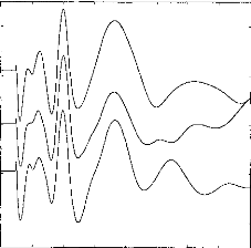
measured peak-to-peak, from a given vertex-positive peak to the following negative peak or through.
Figure 2 shows examples of response averages that appear to be highly reproducible upon visual inspection. Indeed, latencies of waves Ila, Ilb, III, and V appear to be essentially invariant across test runs. The 3x3 cross-correlation matrix confirms the visual impression. Wave amplitudes also are significantly correlated (p<0.001) if the cross-correlation coefficient is higher than 0.2. Intercorrelation is over 0.2 (p<0.001) and the following values have been obtained: 1-2:0.911; 1-3:0.862; 2-3:0.847. The mathematical processing shows a slight shift between the three curves: 1-2:Ops; 1- 3:20ps; 2-3:20ps. Consequently visual examination and mathematical processing lead to a reliable and objective assessment of EABR reproducibility.
0 1 2 3 4 5 6 7 8
Figure 2: EABR reproducibility with three
identical stimulations. Intercorrelation and time shift between
the curves
are: 1-2: 0.911, dT 1-2: 0.00ms ; 1-3: 0.862, dT, 1-3: 0.02ms ; 2-3: 0.0.847,
dT 2-3: 0.02ms.
Amplitude- Intensity Trade-off
Intensity of stimulation, again, can be varied by adjusting amplitude and/or duration of the stimulus pulse (Columbo and Parkins, 1987). These parameters can be controlled independently by the DIGISONIC (fig 3a). Figure 3a shows EABRs evoked by pulses eliciting the same loudness percept in the test subject. In this case, several combinations of amplitudes and durations; the EABRs are quite similar. However,
when amplitude alone is adjusted (figure 3b), an additional wave at 5 ms can be seen with pulses of high amplitude (short duration). In figure 3c, EABRs are plotted for different pulse durations. In figure 3b, no added waves are seen for high intensities. (Note: Loudnesses were the same for corresponding plots of figures 3b and 3c.)
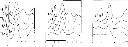
4
3
0 I 2
b:
8
8
3
7
1 2
C.
a:
Figure 3: (3a) Stimulation loudness was equivalent for the 4 curves; with different amplitude and pulse duration. (3b) Thresholds for several stimulation levels (the amplitude of the pulse was modified; stimulation decreased from 1 to 4). (3c) Thresholds for several stimulation levels when the duration of the pulse was modified. Stimulation had the same loudness for corresponding recordings on 3b and 3c (eg 1 and 1).
LII
LIII
LV
d11-111
dIII-V
dll-V
dllp-Iln
dIllp-Illn
dVp-Vn
Ail
A111
AV
Mean
|
Std. dev. |
1 |
2 |
3 |
|
|
1.278 |
0.172 |
NS |
NS |
NS |
|
2.050 |
0.180 |
NS |
NS |
NS |
|
3.864 |
0.276 |
*** |
NS |
NS |
|
0.772 |
0.062 |
*** |
NG |
NG |
|
1.814 |
0.139 |
NS |
NG |
NG |
|
2.586 |
0.156 |
NG |
NG |
NG |
|
0.340 |
0.026 |
NG |
NG |
NG |
|
0.571 |
0.075 |
NG |
NG |
NG |
|
1.074 |
0.102 |
NG |
NG |
NG |
|
0.249 |
0.099 |
NG |
NG |
NG |
|
0.442 |
0.157 |
NG |
NG |
NG |
|
0.590 |
0.163 |
NG |
NG |
NG |
Table II: EABR mean values and standard deviations on 11 subjects, and comparison with other studies (1:Van den Honert and Stypulkowski, 1986; 2:Abbas and Brown, 1988; Kasper et al, 1992). In same cases, our results were compared with other findings using a comparison of mean values (NS: difference being not significant; ***: statistical difference p<0.05; NG: not measured).
RESULTS
EABR--General Characteristics
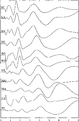
Figure 4: EABR recordings on 11 subjects. Stimulation was on the most apical electrode in the cochlea. Waves II, III and V can be seen for each subject. Y-scale was changed for each subject.
EABRs were recorded successfully for all implantees and all the electrodes leading to an auditory sensation. Ail in all, 58 electrodes were considered, and more than 1000 EABR recording were examined. Figure 4 gives an example of the typical EABR recording obtained. Ail EABR demonstrated similar characteristics with peak latencies as follows: wave II from 0.97 ms to 1.53 ms; wave III from 1.80 and 2.36 ms; wave V from 3.50 and 4.32 ms. An 11x11 correlation matrix of the recordings shown on figure 4 indicates that, apart from some shifts between the subjects, EABRs turn out to be similar across implantees.t If subject SC is Leen as_ a_
reference, following shifts and correlations have been observed: LA:dT=40ps, R=0.83; DN:dT=20ps, R=0.93; DE:dT=260ps, R=0.77; BO:dT=300ps, R=0.89; RO:dT=300ps, R=0.94; LE:dT=580ps, R=0.74; MO:dT=400ps, R=0.86; MA:dT=340ps, R=0.54; FA:dT=700ps, R=0.91; RI:dT=650ps, R=0.65.) Thus, EABR recordings appeared to be reliable and similar among subjects (R>0.2; p<0.001). Average values of latencies, amplitudes, and intervals between wave II, III, and V are indicated on table II. A comparison with the values obtained by others researchers did not show significant differences (Van den Honert and Stypulkowski, 1986; Abbas and Brown, 1988; Kasper et al, 1992).
Effects of stimulation lntensity (Duration)
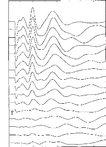
|
2 |
3 |
4 |
5 |
6 |
7 |
8 |
Figure 5: Recordings for one subject: 16 decreasing stimulation intensities were taken. The arrow shows the patient's subjective auditory threshold. Stimulation intensity was controlled by the pulse duration.
In this study again, the primary parameter of stimulus
intensity of interest was the
pulse duration. Figure 5 provides exemplary
data. EABRs could be seen with a very
low stimuli. EABR wave latencies seemed not to be affected by the stimulus intensity. On the other hand, amplitudes were closely linked to the stimulus intensity, as expected. Indeed, the visual detection level of the EABRs was found to correspond well with the threshold of the auditory perception of the stimulus (indicated by the arrow in Fig. 5).
150 200
100
52
3.5 3.0 2.5 2,0 1.5 1.0 0.5
0.0
0
Fig 6 b:
0.5
2.0
0.0
1.5
1.0
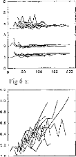
0.8
0.6
0.4
0
0 53
Fig 6 a:
1.2
0.2
1.0
0.0
6
5
3
4
2
"le
100
150 200
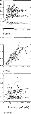
100 150 200
53
Intensity (us/cycle) Fig 6 f:
4.0
·
0.0
0
0 50
Fig 6 d:
100
150
200
3.0
2.5
2.0
1.5
1.0
0.5
0 50 1C0 150 200
Fig 6 c:
|
2.0 1.5 1.0 0.5 0.0 |
52 100 150 200
Intensity (us/cycle) Fig 6 e:
Figure 6: Subject BO: EABR modification with the stimulation intensity given in ps.
(6a) wave II, III, and V latencies.
(6b) d11-111, dIII-V, and dll-V intervals.
(6c) wave II amplitude.
(6d) wave III amplitude.
(6e) wave V amplitude.
(6f) PII-N11, PIII-N111, PV-NV intervals.
Evolution of different EABR parameters, with respect to the stimulation intensity, for a given subject (BO) and on several electrodes is represented on figure 6. Below, p (positive) will indicate the (positive) peak of the wave and n (negative) the valley. Absolute latencies and interpeak intervals were nearly independent of the stimulus magnitude, particularly Ilp-Iln and Illp-Illn. The Vp-Vn interval was observed to increase slightly with increased stimulus intensity.
For each subject, we carried out multiple-linear regression analyses among EABR parameters as a function of stimulus intensity and electrode site. The second column of Table III provides the means and standard deviation (latencies, interpeak intervals and amplitudes) for a change of 100 ps in pulse duration (corresponding to the approximate average dynamic range of stimulation). The third column indicates which values are significantly different from zero. It can be seen, for intense, that lengthening of 100 ps of the stimulus pulse led to decrease of 106 ps of Pll latency. The changes in amplitude for wave II, latency for wave II, and interpeak intervals II- III, III-V, and II-V and not statistically significant. A significant increase of the amplitude of wave III, and V also was seen. Latencies of wave III, & V slightly, but significantly decreased with the stimulation (-106, -200, and -156 ps respectively).
|
Effect of stimulation Intensity |
Effect of Intracochlear Site |
|||
|
Variation per 100 |
p |
Variation per 15 |
p |
|
|
LII (ms) |
-0.212 |
NS |
0.026 |
NS |
|
LIII (ms) |
-0.400 |
0.023 |
-0.022 |
NS |
|
LV (ms) |
-0.312 |
0.013 |
-0.181 |
<0.001 |
|
dl1-111(ms) |
-0.106 |
0.053 |
-0.047 |
NS |
|
dIII-V (ms) |
0.008 |
NS |
-0.157 |
0.004 |
|
dll-V (ms) |
-0.102 |
NS |
-0.161 |
NS |
|
All (pA) |
0.582 |
0.087 |
0.166 |
0.019 |
|
AIII (pA) |
0.848 |
0.019 |
0.363 |
0.040 |
|
AV (pA) |
0.912 |
0.011 |
0.366 |
0.075 |
Table III: Columns 3 and 5: Means and standard deviations (latencies, interpeak intervals and amplitudes) by multiple linear regression for a change of 100 ps in pulse duration and for a change of 15 mm in stimulation site. Columns 4 and 6: Comparison from zero of EABRs variations.
Effects of Stimulated part of the Cochlea
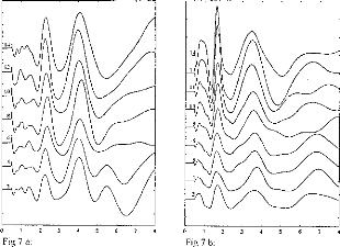
Figure 7: EABR recordings for several electrodes stimulated with the same loudness, for 2 patients. Electrode 1 is basal and electrode 15 is apical.
Figure 7a and 7b demonstrate typical trends in the effects of stimulation electrode/channel, for stimili judged to have the same loudness. The most basal electrode is 2 and the most apical is 14. It can be seen that EABR waveforms were not modified by electrode number or, in effect, stimulus site along the cochlea. Also, wave II, III, and V latencies were similar regardless electrode activated. However, EABR amplitudes were systematically increased when the electrode was moved from base to apex. Data presented in Figure 8 serve to characterize the effects electrode number, for all patients' latencies, amplitudes, and interpeak intervals for waves (II, III, and V). Each point represents the average of the values obtained for different stimulation intensities, (one subject per electrode). The following additional trends are evident:
-wave II latency was not modified with respect to the stimulated zone (fig 8a); -wave V increases from apex to base (fig 8a);
-intervals dIII-V and dll-V decreased with stimulation Gloser to the apex (fig
8b),
-wave II, III, and V amplitudes increased from base to apex (fig 8c, 8d, 8e), as noted before;
-PN intervals for waves II, III, and V were, roughly constant (fig 8f).
|
|
||||||
|
|||||||
|
|||||||
|
|
||||||
|
|||||||
|
|
|
|
||||
|
|||||||
|
|||||||
|
|||||||
|
|
|
|||||
|
|||||||
|
|||||||
|
|
||||||
|
|||||||
|
|||||||
|
|
|
|||||
|
|
||||||
|
|
|
|||||
|
|||||||
|
|
||||||
|
|||||||
|
|||||||
|
|
|
|||||
|
|||||||
|
|||||||
|
|
||||||
|
|||||||
|
|||||||
|
|
|
|||||
|
|
|
|
||||
|
|
|
|
|
|||
|
|
|
|||||
|
|||||||
|
|||||||
0 2 4 6 8 10 12 14 15
Electrode number
16
2 4 6 8 10 12 14
0.0
0 2 4
Fig 8 C:
2.0
6 8 10 12 14 16
Fig 8 a:
0.8
0.6
0.4
0.2
1.6
1.2
0.8
0.4
0.0
0 2 4 6 8 10 12 14 16
Electrode number
|
|
|
|||||||
|
|
||||||||
|
|||||||||
|
|
|
|
|
|
|
|
||
|
|||||||||
|
|
|
|||||||
|
|
|
|
|
|||||
|
|
|
|
||||||
|
|
||||||||
0.5
0
4.5
4
Pt' 4.0
3.5
3.0
2.5
PM 2.0
1.5
1.0.tV
Fig 8 e: Fig 8 f:
Figure 8: EABR values, with respect to the electrode, for all patients. (8a) waves II, III, and V latencies. (8b) d11-111, dIII-V, and dll-V intervals. (8c) wave 11 amplitude. (8d) wave III amplitude. (8e) wave V amplitude. (8f) PII-NII, PIII-N111, PV-NV intervals.
Here too linear regressions were calculated. There fourth column of table III shows the mean and standard deviations of the EABR measures (again, as a function of stimulus duration and electrode site), for a change of 15 mm in stimulation site (corresponding to the depth of penetration of the electrode array. The fifth column indicates which resuits were significantly different from zero. It can be seen, for instance, that lengthening of 15 mm of cochlea led to statistically significant increase
of 26 ps of Pli latency. A significant increase of the amplitude of wave II, III also was seen. Latencies of wave V and interval of waves III-V significantly decreased with the stimulation site(-181, -157 ps). However, the changes of amplitude of wave V, latencies of waves II and III, and interpeak intervals of waves II-III and II-V were not statistically significant.
DISCUSSION
Latencies, amplitudes and intervals measured from waves II, III, and V observed in this study are in good agreement with the values obtained by other researchers (table I). EABRs are composed of at Ieast 3 waves occurring within a time shorter than 6 ms. Wave II, with its bifid shape (Van den Honert, 1986), was seen in all the subjects. Wave Ila is probably wave I because its latency is similar to the auditory nerve compound action potential latency (Brown and Abbas, 1990; Gantz et al, 1994). Wave III was observed to have a relatively high amplitude and short duration. The IV- V complex was wider than the other waves, as characteristic of the acoustically evoked response. It has been suggested (Abbas and Brown, 1988, 1991a) that the stimulation of the basal part of the cochlea triggers a wide spread excitation. This was not seen with our technique.
Although EABRs stimulated in base of the cochlea are difficult to record (Shallop et al, 1993), it was possible in this study to obtain and label EABRs for all electrodes (within and across subjects) capable of eliciting an auditory sensation. Consequently waves II, III, and V latencies, amplitudes, and intervals were measured. We believe that the high quality of our EABR recordings was due to the shape of the stimulation pulse (asymmetry, sharp positive phase and short duration pulse for low-level), leading to good synchronization, and our method of digital processing of the data, leading to robust suppression of artifacts.
Average values calculated in our study were in agreement with those given by other investigators. However, they may be far different from usual values measured on healthy subjects as it seems likely that wave latency reflects the effects of limited populations of primary auditory neurons and/or auditory deprivation prior to implantation (Gallégo et al, submitted c). For healthy subjects, waves latencies should be close of those seen for SC, DN, and LA (L11=1.10ms, 1111=1.85 ms,
LV=3.55 ms). Regardless of the variability among subjects, EABR shapes were reasonably stationary in time; intersubject correlation was always higher than 0.2 (p<0.001).
Choice of Stimulus Parameters and Effects of Stimulus Intensity/Duration
As stated earlier, electrical stimulation can be controlled by two means, pulse amplitude (figure 3b) and duration (figure 3c). Amplitude is the most commoniy used parameter in examining the EABR. The problem with adjusting amplitude is that at high intensities, the spread of excitation within in cochlea effectively increases and may even corne to involve the vestibule and facial nerve. The use of the pulse duration bears several advantages, as suggested earlier and verified by the results reported here. The results in Figure 3 demonstrate the comparability of results obtained with stimuli of the same intensity, regardless of parameters. However, for EABR, when amplitude is high and duration short, a wave, probably myogenic (Fifer and Novak, 1990), is seen with a latency of 5 ms approximately (e.g. see figure 3b). Consequently, the use of pulse duration, rather than magnitude to control stimulation intensity is likely to improve the quality of the recording and to simplify the interpretation. The results suggest further that, ineed, using pulse duration, the stimulated zone on the cochlea remains constant. Even with low-intensity stimulation (i.e. decreased duration), synchronization is facilitated (fig. 3c).
Several authors (Allum et al, 1990; Abbas and Brown, 1991a; Shallop et al, 1990, 1991, 1993) have found an increase in latency for low levels of stimulation; others (Van den Honert and Stypulkowski, 1986; Kasper et al, 1991, 1992) found latencies to be essentially invariant. None of the studies considered pulse duration in order to control the stimulation. In our work, stimulation duration had an average of 54.5ps (s.d. 36.25ps). The mean range was around 100 ps. We observed a constant of latencies and interpeak intervals with stimulation intensity (i.e. ranges were -212ps=- 16.5% for wave II, -400ps= -19.5% for waves Ill, and -312ps= -8.1% for wave V).
Still other investigators have considered the influence of shape of the stimulus pulse
(Rattay, 1987), the evoked response elicited by the negative phase (Moxon, 1971;
Javel, 19861 and refractory period (Abbas and Brown, 1991 b; Kasper et al, 1992).
Rattay showed that the steeper the slope of the electrical pulses, the better the synchronization of the 8th nerve response. Both Moxon and Javel noted that when the electrical stimulation biphasic pulse was wide, auditory neurons could respond on the second phase. Durational effects also relate to the refractory period of neurons. One of the consequences of this phenomena is that EABR thresholds were correlated to perceptual thresholds (Gallégo et al, 1996,1997a; Truy et al, 1997a,b) than with other stimulation strategies (Shallop et ai, 1991, 1993; Brown et al, 1994; Mason et al, 1994; Smith et al, 1994). Propagation speed appeared to be increased for strong stimulation, but the variation is compared to ABR amplitude, and intervals between the waves turned out to be unrelated to the stimulation intensity.
Effect of Cochlear Region of stimulation
It has been noted (Black et al, 1983; O'Leary et al, 1985) that with bipolar stimulation, the stimulated segment on the cochlea can be very small (voltage distribution is divided by three for a distance from 2 to 4 mm). Studies in animais show a high correlation between the response and the frequency-place excitation parameters in the inferior colliculus (Black and Clark, 1980). Variation of latency, interpeak intervals and amplitudes of waves II, Ill, and V versus the stimulated electrode were measured in the present study (fig 6). The latency of wave II was not found to be dependent upon the stimulated zone. Therefore there is no tonotopic influence upon the timing of neural discharges reaching (i.e. unlike the case of acoustic ABR). This result is in agreement with previous histological studies (Hinojosa et al, 1985; Spoendlin et al, 1972, 1988 ; Moore, 1987a ; some extend, Spoendlin, 1989) which failed to show any substantive/systematic variations in nerve fiber diameter as a function of tonotopic origin in the cochlea. This also is consistent with electrically stimulated single-unit responses (Kiang and Moxon, 1972).
Generally, wave V latency (in agreement with Miller et al, 1993) and the III-V interval was found to decrease from base to apex. Also, information processing appeared to be faster, from the exit of the cochlear nucleus to the last nuclei of the brain stem, for low-frequency compared to the high-frequency places of stimulation. This apparent increased efficiency of transmission along the brain stem amounted to roughly 0.18 ms (4.7%) for wave V tatencies (cochlea to inferior colliculus) and 0.16 ms (8.8%) for
waves III-V interval (cochlear nucleus to inferior colliculus) for a corresponding distance of 15 mm along the cochlea.
Wave amplitudes in this study were found to be higher with more apicalward stimulation (end of the first turn); width of the waveform, however, was roughly constant. It has been observed that the transfer functions of the auditory nerve fibers is essentially the same from base and apex (Kiang and Moxon, 1972). The modification of the amplitude cannot be explained by desynchronization of the fibers. An explanation, however, can be offered via results of the following studies: -in the human and in the cat a correlation has been reported between EABR amplitude, and the number of cells in spiral ganglion (Smith and Simmons, 1983; Hall, 1990); -in both the cat (Spoendlin, 1972) and in normal humans (Hinoja et al, 1985; Spoendlin and Schrott, 1988, 1989), histological studies have showed an increase of cell density in the spiral ganglion, from the base to the end of the first cochlear turn. The low amplitude of the waves, at the base, could be directly connected to a lower number of cells on the spiral ganglion. For some subjects, however, the amplitude did not vary monotonically from base to apex. The effect thus may depend on the etiology of deafness, as since some authors noted a correlation between number of spiral ganglion cells and the nature of the auditory loss (e.q. Otte et al, 1978; Schmidt, 1985).
ACKNOWLEDMENTS
The authors acknowledge persons and institutions who supported their work: the MXM company, the CIFRE, the Hospices Civils of Lyon, the CNRS, the University of Lyon, professor Alain Morgon (head of the ORL department), and the eleven implantees who participated in this study.
REFERENCE
Abbas PJ, Brown CJ. Electrically evoked brainstem potentials in cochlear implant patients with multi-electrode stimulation. Hear Res 1988 36:153-62
Abbas PJ, Brown CJ. Electrically evoked auditory brainstem response: Growth of the response with current level. Hear Res 1991a 51:123-37
Abbas PJ, Brown CJ. Electrically evoked auditory brainstem response: Refractory properties and strength duration functions. Hear Res1991b 51:138-48.
Allum JHJ, Shallop JK, Hotz M, Pfaltz CR. Characteristics of electrically evoked 'auditory' brainstem responses elicited with the Nucleus 22-electrode intracochlear implant. Scand Audiol 1990 19:263-7
Arnold SA. Objective versus Visual Detection of the Auditory Brain Stem Response. Ear Hear 1985 6(3):144-50
Beliaeff M, Dubus P, Leveau J-M, Repetto J-C, Vincent P. Sound Signal Processing and
Stimulation Coding of the DIGISONIC DX10 15-Channel Cochlear Implant. Advances in Cochlear Implant Ed Hochmair-Desoyer IJ & Hochmair ES Innsbruck 1994 198-203
Black R, Clark GM. Differencial electrical excitation of the auditory nerve. J Acous Soc Am 1980 67:868-74.
Black R, Clark G, Tong Y, Patrick J. Current distributions in cochlear stimulation. Ann NY Acad Sci 1983 405:137-45
Brightwell A, Rothera M, Conway M, Graham J. Evaluation of status of the auditory nerve: psychophysical test and ABR. Eds RA Schindler & MM Merzenich Cochlear Implants Raven Press New York 1985 343-9
Brown CJ, Abbas PJ. Electrically evoked whole nerve action potentials: Data from human cochlear implant users. J Acoust Soc Am 1990 88(3):1385-91
Brown JB, Abbas PJ, Fryauf-Bertschy H, Kelsay D, Gantz BJ. Intraoperative and Postoperative Electrically Evoked Auditory Brain Stem Responses in Nucleus Cochlear Implant Users: Implications for the Fitting Process. Ear Hear 1994 15:168-76
Bruce JG, Brown CJ, Abbas PJ. Intraoperative measures of electrically evoked auditory nerve compound action potential. Am J Otology 1994 15(2):137-44
Busby PA, Tong YC, Clark GM. Electrode position, repetition rate, and speech perception by early- and late-deafened cochlear implant patients. J Acoust Soc Am 1993 93(2):1058-67 Chouard CH, Ouayoun M, Meyer B, Fugain C. Speech Coding Strategies of the DIGISONIC Fully Digitized Cochlear Implant. Acta Otolaryngol (Stockh) 1995 115:264-8
Clark GM, Tong YC, Martin LFA. A multiple-channel cochlear implant: an evaluation using closed-set spondaic words. J Laryngol 1981 95:461-4
Clark G, Shepherd R, Franz B, Dowell R, Tong Y et al. The histopathology of the human temporal bone and auditory central nervous system following cochlear implantation in patient. Acta Otolaryngol (Stockh) 1988 (suppl 448):1-65
Clopton B, Spelman F. Neural mechanisms relevant to the design of an auditory prothesis: location and electrical characteristics. Ann Otol Rhinol Laryngol 1982 91(sup98):9-14 Columbo J, Perkins CW. A model of electrical excitation of the mammalian auditory nerve neuron. Hear Res 1987 31:287-312
Don M, Eggermont JJ. Analyses of click-evoked brainstem potentials in man using high-pass noise masking. J Acoust Soc Am 1978 63(4):1084-98
Don M, Ponton CW, Eggermont JJ, Masuda A. Gender differences in cochlear response time: An explanation for gender amplitude differences in the unmasked auditory brain-stem response. J Acoust Soc Am 1993 94(4):2135-48
Don M, Ponton CW. Auditory brainstem response (ABR) peak amplitude variability reflects
individuel differences in cochlear response times. J Acoust Soc Am 1994 96(6):3476-91 Durrant JD. Fundamentals of sound generation. Bases of Auditory Brain-Stem Evoked Responses (Ed EJ Moore) Grune et Stratton Inc New York 1983 15-50
Eddington DK. Speech discrimination in deaf subjects with cochlear implants. J Acoust Soc Am 1980 51:885-91
Eggermont J. Analysis of click-evoked brainstem potentials in humans using high-pass noise masking.lI. Effect of click intensity. J Acoust Soc Am 1980 68:1671-5
Fifer RC, Novak MA. Myogenic Influences on the Electrical Auditory Brainstem Response (EABR) in Humans. Laryngoscope 1990 100:1180-4
Gallégo S, Micheyl C, Berger-Vachon C, Truy E, Morgon A, Collet L. Ipsilateral ABR with cochlear implant. Acta Otolaryngol (Stockh) 1996 116:228-33.
Gallégo S, Truy E, Morgon A, Collet L. EABRs and surface potentials with a transcutaneous multielectrode cochlear implant. Acta Otolaryngol (Stockh) 1997a 117:164-8.
Gallégo S, Collet L., Berger-Vachon C. Electrically auditory brainstem responses (EABR) : contribution of a filter adapted to the auditory system. J international federation for medical & biomedical engineering, 1997b, 35 (suppl 1), 304.
Gallégo S, Garnier S, Berger-Vachon C. Traitement du signal de parole pour sourds-profonds: l'implant cochléaire. Revue d'électricité et d'électronique. 1997c, 8, 50-53.
Gallégo S, Collet L., Berger-Vachon C. A model of electrical stimulation delivered by the Digisonic cochlear implant. J international federation for medical & biomedical engineering, 1997d, 35 (suppl 1), 300.
Gallégo S, Lu BL, Berger-Vachon C. Modelling of the electrical stimulation delivered by the DIGISONIC Multichannel cochlear implant. Advance in Modelling & Simulation Eng 1997e, in press.
Gallégo S., Frachet B., Truy E., Collet L. Cochlear implant performance and electrically auditory brainstem response characteristics. (in press)
Gallégo S, Beliaeff M, Frachet B, Berger-Vachon C, Collet L. Long-term change in threshold and
comfort levels and dynamics in Digisonic cochlear implant bearers. Submitted a.
Gallégo S, Durrant J, Collet L., Berger-Vachon C. Numeric time-variant filters adapted to the
recording of electrically auditory brainstem responses (E-ABR). Submitted b.
Gallégo S, Truy E, Berger-Vachon C, Collet C. Electrically auditory brainstem responses in cochlear implant assessment: possibility and interest. Submitted c.
Gantz BJ, Brown CJ, Abbas PJ. Intraoperative measures of ellectrically evoked auditory nerve compound action potential. Am J Otol 1994 15:2 137-44
Gorga MP, Kaminski JR, Beauchaine KA, Jesteadt W. Auditory brainstem responses to tone bursts in normally hearing subjects. J Speech Hear Res 1988 31:87-97
Greenwood DD. A cochlear frequency-position function for several species-29 years later. J Acoust Soc Am 1990 87(6):2592-605
Gronfors T, Juhola M. Effect of sampling frequencies and averaging resolution on medical
parameters of auditory brainstem responses. Comput Biol Med 1995 25, 5:447-54
Gyo K, Yanagihara N. Electrically and acoustically evoked brainstem responses in guinea pig.
Acta Otolaryngol (Stockh) 1980 90:25-31.
Hall RD. Estimation of surviving spiral ganglion cells in the deaf rat using the electrically evoked auditory brainstem response. Hear Res 1990 45:123-36
Hinojosa R, Seligsohn R, Lerner S. Ganglion cell counts in the cochleae of patients with normal audiograms. Acta Otolaryngol (Stockh) 1985 99:8-13
House WF, Berliner K, Crary W, Graham M, Luckey R, Norton N, Selters W, Tobin H, Urban J, Wexler M. Cochlear implants. An Otol Rhinol Laryngol 1976 85(suppl 27):1-93
Javel E. Basic response properties of auditory nerve fiber. Neurobiology of Hearing: The
Cochlea. 1986 Ed Altschuster RA, Bobbin RB, Hoffman DW. Raven Press. New York.
Javel E, Tong Y, Shepherd B, Clark G. Responses of cat auditory nerve fibers to biphasic electrical current pulses. Ann Otol Rhinol Laryngol 1987 96(suppl 128):26-30
Jewett DL, Williston JS. Auditory evoked far-fields averaged from the scalp of humans. Brain 1971 94:681-96
Kasper A, Pelizzone M, Montandon P. Electrically Evoked Auditory Brainstem Responses in Cochlear Implant Patients. ORL 1992 54:285-94
Kasper A. Electrically Evoked Activity in Human Auditory System. Thesis 1991 Genève.
Keitley EM. Frequency map of the spiral ganglion in the cat. J Acoust Soc Am 1987 81(4):103642
Kiang NYS, Moxon EC. Physiological considerations in artificial stimulation of the inner ear. Ann Otol Rhinol Laryngol 1972 81:714-31
Leake PA, Snyder RL. Topographic organisation of the central projections of the spiral ganglion in cats. J Comp Neurol 1989 281:612-29
Mason S, Sheppard S, Garnham C, Lutman M, O'Donoghue, Gibbin K. Improving the relationship of intraoperative EABR threshold to T-level in young children receiving the Nucleus cochlear implant. Advances in Cochlear Implant Ed Hochmair-Desoyer IJ & Hochmair ES 1994 44-49.
Michelson RP. Electrical stimulation of human cochlear: A preliminary report. Arch Otolaryngol 1971 93(3):317
Miller CA, Abbas PJ, Brown CJ. Electrically evoked auditory brainstem response to stimulation of different sites in the cochlea. Hear Res 1993 66:130-42
Moore JK. The human auditory brainstem: A comparative view. Hear Res 1987a 29:1-32
Moore JK. The human auditory brainstem as a generator of auditory evoked potentials. Hear Res 1987b 29:33-43
Moxon EC. Neural and mechanical responses to electric stimulation of the cat's inner ear. Thesis. 1971 MIT Cambridge, Mass.
O'Leary S, Black R, Clark G. Current distributions in the cat cochlea: a modelling and electrophysiological study. Hear Res 1985 18:273-81
Otte J, Schuknecht H, Kerr A. Ganglion cell populations in normal and pathological human
cochleae. Implications for cochlear implantation. Laryngoscope 1978 88:1231-46
Pfingst BE, De Haan DR, Holloway LA. Stimulus features affecting psychophysical detection thresholds for electrical stimulation of the cochlea.1: Phase duration and stimulus duration. J Acoust Soc Am 1991 90(4):1857-66
Rattay F, Motz H. Stimulation of a multichannel nerve array to pulse shapes produced by a single channel electrostimulation. Perception 1987 16:769-76.
Rosbe KW, Burgess BJ, Glynn RJ, Nadol JB. Morphologic evidence for three cell types in the human spiral ganglion. Hear Res 1996 93:120-7
Schmidt J. Cochlear neuronal populations in developmental detects of the inner ear:
implications for cochlear implantation. Acta Otolaryngol (Stockh) 1985 99:14-20
Shallop JK, Beiter AL, Goin DW, Mischke RE. Electrically Evoked Auditory Brain Stem Responses (EABR) and Middle Latency Responses (EMLR) Obtained from Patients with the Nucleus Multichannel Cochlear Implant. Ear Hear 1990 11,1:5-15
Shallop JK, VanDyke L, Goin DW, Mischke RE. Prediction of behavioral threshold and confort values for Nucleus 22-channel implant patients from electrical auditory brain stem response test results. Ann Otol Rhinol Laryngol 1991 100:896-8
Shallop JK. Objective electrophysiological measures from cochlear implants patients. Ear Hear 1993 14:58-63
Simmons FB. Electrical stimulation of the auditory nerve in man. Arch Otolaryngol 1966 84:2-54 Smith DW, Finley CC, Van den Honert C van den, Olszyk VB, Konrad KEM. Behavioral and electrophysiological responses to electrical stimulation in the cati. Absolute thresholds. Hear
Res 1994 81:1-10
Smith L, Simmons FB. Estimating eighth nerve survival by electrical stimulation. Ann Otol Rhinol Laryngol 1983 92:19-23
Sohmer H, Feinmesser M. Cochlear action potentials recorded from the external ear in man. Ann Otol Rhinol Laryngol 1967 76:427-35
Spoendlin H. Innervation densities of the cochleae. Acta Otolaryngol (Stockh) 1972 73:235-48 Spoendlin H, Schrott A. The Spiral Ganglion and the Innervation of the Human Organ of Corti. Acta Otolaryngol (Stockh) 1988 105:403-10
Spoendlin H, Schrott A. Analysis of the human auditory nerve. Hear Res 1989 43:25-38
Starr A, Brackman DE. Brainstem potentials evoked by electrical stimulation of the cochlea in human subjects. Ann Otol Rhinol Laryngol 1979 88:550-60
Truy E, Gallégo S, Berger-Vachon C, Morgon A. Multichannel cochlear implant in patients with ossified cochlea. Interest of the optimization of frequential selectivity of speech signal with Digisonic device. Proc IlIrd int Symp Transplants & implants in otology. Bordeaux (France), June 10-14 1995. M portman, P. Boudard, D. Portman, pp. 399-402.
Truy E, Gallégo S, Channal JM, Collet L, Morgon A. Correlation between electrical auditory brainstem response and perceptual thresholds in Digisonic cochlear implant. Laryngoscope 1997a, 117: in press.
Truy E, Gallégo S, Channal JM, Collet L, Berger-Vachon C, Morgon A. Intérêt des potentiels évoqués auditifs électriques du tronc cérébral chez les patients porteurs d'un implant cochléaire digisonic. Ann Otolaryngol Chir Cervicofac, 1997b, 114, 116-124.
Van den Honert C, Stypulkowski PH. Physiological properties of the electrically stimulated auditory nerve.11. Single fiber recording. Hear Res 1984 14:225-43
Van den Honert C, Stypulkowski PH. Characterization of the electrically evoked auditory brainstem response (ABR) in cats and humans. Hear Res 1986 21:109-26
Waring MD. Electrically evoked auditory brainstem response monotoring of auditory brainstem
implant integrity during facial nerve tumor surgery. Laryngoscope 1992 102:1293-5
Waring MD. Auditory brain-stem responses by electrical stimulation of the cochlear nucleus in
human subjects. Electroenceph clin Neurophysiol 1995 96:338-47
Zapala DA, Gould HJ, Mendel MI. Place specific influence on the wave I to V interpeak latency of the auditory brain-stem response. J Acoust Soc Am 1992 92(6):3174-84
Des résultats obtenus en psychophysique ont montré de grosses modifications des seuils d'inconforts et dynamiques en fonction du temps d'implantation, ce qui sous-entend une plasticité du système auditif. Des travaux chez l'animal ont montré par les PEAEP (Miller et al, 1995a,b) et/ou les CAP (de Sauvage et al, 1997) des modifications électrophysiologiques au niveau des seuils d'apparition et de l'amplitude des réponses.
Nous avons voulu étudier, les possibles modifications des latences des PEAEP en fonction du temps chez une population de 9 implantés cochléaires Digisonic. En effet une modification des amplitudes en fonction de l'intensité de stimulation ne ferait que refléter l'évolution des dynamiques ; par contre des modifications de latences sous-entendraient des modifications au niveau du temps de conduction ainsi que du temps de traitement par le système auditif de l'information.
Les résultats présentés figure 99 décrivent les modifications des latences des PEAEP à un an d'intervalle. Chaque valeur représente une moyenne d'une trentaine de PEAEP. Aucune différence statistique n'a été trouvée pour les latences des ondes III et V. Une étude plus rigoureuse prenant les sujets implantés cochléaires de JO jusqu'à J600 serait peut être plus démonstrative. En tout cas, cette pré-étude n'a pas montré de changements très flagrants des caractéristiques des PEAEP, ce qui nous a encouragé à développer la technique de recueil de PEAEP avant l'implant par une stimulation extra- cochléaire.
Un couplage entre l'étude des modifications psychophysiques (tonie/sonie) et l'étude des caractéristiques des PEAEP semble néanmoins très prometteur.
Figure 99 : Latences des ondes III et V des PEAEP et durée d'implantation chez 9 sujets implantés.
dl Faisabilité en préimplantation
L'utilisation des PEAEP avant l'implantation paraît aussi intéressante celà soulève des problèmes
supplémentaires. La mise place d'une technique et d'un protocole adapté semble nécessaire.
S. Gallégo, E. Truy, C Berger Vachon, L. Collet
Article soumisL'étude consiste à étudier la faisabilité du recueil de potentiels évoqués auditifs électriques précoces (PEAEP) avec une électrode temporaire de stimulation. Dans un premier temps l'étude de la littérature a permis de confirmer la faisabilité physiologique et technique des PEAEP lors d'une stimulation électrique de la fenêtre ronde ou du promontoire. Il a ainsi été possible de définir un protocole d'enregistrement des PEAEP (position des électrodes de stimulation et de recueil, paramètres d'acquisition, traitement numérique post-acquisition). Pour finir, des résultats préliminaires sur 9 cas ont été décrits. L'optimisation de la technique a permis d'obtenir des PEAEP dans 78 % des cas.
Malgré les contraintes techniques et physiologiques, les PEAEP peuvent être enregistrés avec une électrode temporaire sur la fenêtre ronde. Le positionnement, le choix des électrodes de recueil et de stimulation ainsi que le traitement numérique post-acquisition sont très important pour obtenir des PEAEP pré-implantation. Cette technique ne peut être actuellement que consultative car elle n'est fiable que dans 78 % des cas. Les résultats obtenus nous encouragent cependant à la développer et à l'étendre à une stimulation du promontoire au lieu de la fenêtre ronde. L'enjeu est en effet important, l'utilisation de cette méthode donnerait des éléments objectifs qui appuieraient une décision d'implantation, aideraient à choisir le côté à implanter et permettraient de faire une estimation des performances du sujet après l'implantation.
ELECTRICALLY AUDITORY BRAINSTEM RESPONSES IN COCHLEAR IMPLANT
ASSESSMENT : POSSIBILITY AND INTEREST.S. Gallégo, E. Truy, C. Berger-Vachon, L. Collet
UPRESA- CNRS 5020 & MXM laboratoryABSTRACT : The present study is the feasibility of recording electrically auditory brainstem responses (EABR) with a temporary stimulating electrode. Preliminary study of the literature confirmed the physiological and technical feasibility of EABR with electro-stimulation of the round window or of the promontorium. This enabled a EABR recording design to be drawn up: stimulating and recording electrode positions, recording parameters and post-recording and data processing. Finally, preliminary results for 9 cases are described. Optimising the technique enabled EABRs to be recorded in 78 % of cases.
Key words: EABR, prior implantation test, Cochlear Implant. INTRODUCTION
Developments in signal processing and encoding strategy for the various cochlear implant (CI) now enable very good clinical results to be obtained. The percentage of `star patients' (able to communicate by telephone using only auditory information) is steadily growing. Even so, Cl subject performances remain variable and are not totally predictable or accounted for.
It is generally accepted that Cl bearers' pre-implantation performance can be assessed in terms of parameters such as length of sensory deprivation, aetiology of defect, language level, lip-reading performance, psycho-physical performance, IQ, motivation, family back ground, ... Measuring auditory remains (neurone population) is also a key-factor for Cl prognosis. There at present few tests of auditory system functioning. Lusted et al (1984), Shannon (1983) and Pfingst et al (1980, 1984) have shown threshold and comfort levels and dynamics in implanted subjects to be closely dependent upon aetiology and spiral ganglion neurone population.
The commonest means of assessing the remaining neurone population is by measuring threshold and comfort levels using electrical stimulation of the round window or of the promontorium by a temporary electrode (House et al, 1976; Shipp et al, 1991). This test is, however, unreliable and open to criticism, in that only positive results can be validated. Response failure or defective levels are not necessarily indicative of an auditory system defect, but could simply be due to faulty stimulation electrode positioning or poor electrical diffusion in the physiological environment of the cochlea. Moreover, the test is hard to conduct in children or in poorly conditioned adult subjects, requiring as it does considerable patient participation.
Error in predicting Cl performance are partly due to the lack of objective measurements of the state of the auditory system. Electrophysiology (i.e., evoked potentials could provide a means of objectifying measurement so as to better quantify neurone population and the functional state of the auditory system.
The present study used electrical stimulation of the cochlea by a temporary electrode on the promontorium or the round window to study the technical and physiological feasibility and the usefulness of pre-implantation EABR recording.
Interest of pre-implantation EABR recording
There are several studies in the literature which wouid encourage the idea of using pre-implantation EABRs as a means of predicting post-implantation performance. Certain authors (Wesber and Wesber, 1979; Chouard et al, 1983) have reported correlation between duration of deafness and auditory system neurone population. Acoustic stimulation studies (Otte et al, 1978; Schmidt et al, 1985) have correlated deaf subjects' hearing loss to spiral ganglion cell number. Pauler et al (1986) found a correlation between intelligibility and spiral ganglion neurone population. Measuring auditory system neurone density wouid thus allow an estimation of performance.
Studies in animais (Hall et al, 1990) and in humans (Smith et al, 1983; Brighwell et al, 1985) have shown correlation between spiral ganglion neurone population and ABR amplitude under electrical stimulation (EABR). Other authors (Gallégo et al, 1997) have correlated recognition without lip-reading in Cl-bearers to certain EABR parameters (wave Ill and V latency interval). EABR thus do enable estimation of auditory system neurone population and Cl-bearers' performance..
Systematic pre-implantation EABR recording would thus enable measurement of auditory system functionaiity, estimation of its neurone population, and prediction of performance with Cl. This could heip in decision to implant, choice of implant-side, type of implant (mono- or multi-channel) and of implant encoding strategy (slow or fast stimulation).
Physiological and technical constraints
Electrical stimulation to the base of the cochlea through an extra-cochlear temporary electrode can produce auditory sensations. The stimulating electrode may be placed either on the promontorium or on the round window, and the techniques in the two cases are not the same. For positioning on the promontorium , a transtympanic electrode is slipped through, without any need of anaesthetic. Round window positioning requires lifting the tympanum and a local anaesthetic. According to the literature (Shipp et al, 1991), perceptual threshold measurements and test reliability are better with a round window design; ciinical and ethical problems, however, arise, given the need for surgery and local anaesthesia. EABR recording using a promontory stimulating electrode has the advantage of being less invasive, even if technically less simple to make (the electric currents are weaker and better focussed on the cochlea with round-window stimulation). Developing EABR recording techniques using a temporary stimulating electrode therefore needs to start off from round-window stimulation to end up if possible with promontorium design.
Does electrical stimulation of the base of the cochlea generate EABR?
EABRs can be recorded from ail the Cl electrode, even the most basal (Gallégo et al, 1996, 1997). Thus very basal stimulation can indeed generate EABRs (even if the number of cochiear neurones thus excited is less than for more apical stimulation). This increases the difficulty of recording, by increasing adaptation (the smaller the number of excited neurones the greater their adaptation) and decreasing the signalto-noise ratio). With Cl, EABR intensity is always below comfort level threshold (Abbas and Brown, 1988; Shallop et al, 1991; Gallégo et al, 1997), which makes recording possible without anaesthetic.
Extracochlear evoked responses
With temporary electrodes, electrical stimulates diffuses widely in the tissue. Nonauditory responses can thus easily overlay EABRs. Fifer et al (1990) have described myogenic responses, producing fairly high amplitude waves with 5-7 ms latency, which badly disturb EABR recording, masking as they do wave V.
Gyo et al (1980) and Honert and Stypulkowski (1986) have also demonstrated the possibility of vestibular responses during the first milliseconds, although the latencies and amplitudes of these waves in human have not been accurately determined. Electrical stimulation can further activate the facial and buco-pharyngeal nerves, disturbing recording by saturating the entry amplifier of the acquisition system.
Subjects
Nine subjects took part in the present study (2 children, 7 adults). All had presented for conventional pre-implantation electrical testing. AIl had profound or total bilateral deafness. Testing took place without anaesthetic for 5 of adults and under general anaesthetic for 4 subjects (2 children, 2 adults).
TECHNICAL SET-UP
Positioning of stimulating and recording electrodes
To limit stimulus artefact, electrical diffusion in the physiological environment needs to be kept to a minimum. One way doing this is to localise stimulation by bringing the two stimulating electrodes as close as possible (the positive on the round window, the negative behind the ear on the petrosal). To limit extracochlear stimulation (myogenic, vestibular, buco-pharyngeal and facial nerve), the positive electrode is small, to focus on the cochlea, and the negative one large, to diffuse the current outside the cochlea, reducing charge per area. The current thus flows horizontally. To reduce stimulus artefact, recording electrodes are placed perpendicularly to the current flowline: positive on the forehead, negative on the chin (see fig. 1). The earth is placed on the contralateral earlobe.
Figure 1: Synopsis of stimulating and recording electrode positions. The axis formed by the stimulating electrodes was perpendicular to that formed by the recording electrodes (AB perpendicular to CD). The stimulation axis (AB) projects across the middle of the recording segment (CD).
I deally, if the distances between the stimulus and the positive and negative
recording electrodes are equivalent (AD=AC), and if the angle between the recordingand the stimulating electrodes is 90°, then the stimulus artefact cancels out in the recording.
Stimulator
The electrical stimulator was a prototype (Digistim+ system) developed by the MXM company, which can send two phase pulsed stimulation controlled for current, pulse duration and frequency, and can synchronise the EABR recording system.
Recording parameters
The system recorded EABRs over 10 ms at a sampling frequency of 50 kHz. Fullscale sensitivity was +1- 50 iiV. The analogic input filter was 0.2-8,000 Hz. Each recording corresponded to an averaging of 512 sweeps, was safeguarded then transferred onto a PC for post-recording digital analysis.
Post-recording digital analysis
Post-recording digital filtering is a good way of enhancing EABR curves, although conventional post-recording digital filters do not work well as they also filter stimulus artefact effects. The digital filter used here is specially adapted to auditory system functioning and electrical stimulation requirements (Gallégo et al, submitted). The frequencies in each wave have been shown to grow lower as wave latency lengthens. The idea of the filter is to vary the transfer function according to the latency. Simulations have shown this digital filtering to be able to reveal a EABR with a signal-to-noise ratio of --36dB (noise some 60-foid stronger than signal); hence it can also reduce non-auditory waves and stimulus artefact derivatives.
Results and discussion
Figure 2 shows a typical case, with the EABR overlain by a myogenic response. The wave V amplitude (around 4 ms) was much lower than the myogenic wave's (around 6 ms). In this case, a needle electrode had been used as negative stimulating electrode: focussing the current between the round window and petrosal bone, it encouraged extracochlear myogenic stimulation.
o
9 10
Figure 2: Example of EABR with a myogenic response. Wave V latency is 4.05 ms. Myogenic wave
latency is around 6 10 ms.
Figure 3 gives an example of EABRs recorded from a non-anaesthetised adult
subject when electrode positions and recording parameters have been optimised.
Waves III and V are easily identifiable. The EABR wave forms and latencies are very
similar to those found after implantation. 1.0
0.5
0.0
>
-0.5
N
-"C:7 = :'-' -1.0
Q
E
< -L5
- 2.0
- 2.5 0 0 0.5 1.0 1.5 2.0 2.5 3.0 3.5 4.0 4.5 5.0 5.5 5 0
Latence (ms)
Figure 3: Example of EABR on non-anaesthetised subject. Wave V Iatency is 4.15 ms. Wave III Iatency is 2.35 ms.
Figure 4 is an example of EABRs from a child subject under general anaesthetic just before implantation. Wave V is easily identifiable, but not wave III.
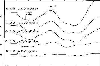
0 1 2 3 4 5 6 7 8
Ti me (ms)
Figure 4: Example of threshold of EABR on general anaesthetised child. Wave V Iatency is 4.00 ms.
Out of 9 subjects tested, EABRs were obtained in only 7 cases
(78 % success rate).
Wave was aiways identifiable, but wave III only in 4
cases. Mean of wave V Iatency is
4.15 ms (S.D = 0.30 ms). Mean of wave V Iatency is 2.25 ms (S.D = 0.25 ms). Resuits are approximately the same of Cochlear Implant (Gallégo et al, 1996, 1997).
CONCLUSION
Despite technical and physiological constraints, EABRs can be recorded with a temporary electrode on the round window. Positioning and choice of recording and stimulating electrodes, and post-recording digital processing, are all very important in obtaining pre-implantation EABRs. The technique, with only 78% reliability, is as yet of only consultative value, but the results here nevertheless encourage development and its extension to promontory rather than round window stimulation. The stake is high: being able to use this method would give objective support to indications for implantation, help choose the implant side and enable estimation of subject's' post- implantation performance.
REFERENCES
Abbas PJ, Brown CJ. Electrically evoked brainstem potentials in cochlear implant patients with multi-electrode stimulation. Hear Res 1988; 36:153-62.
Brightwell A, Rothera M, Conway M, Graham J. Evaluation of status of the auditory nerve: psychophysical test and ABR. Eds RA Schindler & MM Merzenich Cochlear Implants Raven Press New York 1985 343-349.
Chouard CH, Josset P, Meyer B, Buche JF. Effect of chronic electrical stimulation of the auditory nerve on development of cochlear nuclei in guinea-pig. Ann OtolLaryngol (Paris) 1983; 100:417-422.
Clark G, Shepherd R, Franz B, Dowell R, Tong Y et al. The histopathology of the human temporary bone and auditory central nervous system following cochlear implantation in patient. Acta Otolaryngol (Stockh) 1988; (suppl 448):1-65.
Fifer RC, Novak MA. Myogenic Influences on the Electrical Auditory Brainstem Response (EABR) in Humans. Laryngoscope 1990; 100:1180-1184.
Gallégo S, Micheyl C, Berger-Vachon C, Truy E, Morgon A, Collet L. Ipsilateral ABR with cochlear implant. Acta Otolaryngol (Stockh) 1996; 116:228-233.
Gallégo S, Truy E, Morgon A, Collet L. EABRs and surface potentials with a transcutaneous multielectrode cochlear implant. Acta Otolaryngol (Stockh) 1997; 117:164-168.
Gallégo S, Durrant J, Collet L., Berger-Vachon C. Numeric time-variant filters adapted to the recording of electrically auditory brainstem responses (E-ABR). Submitted.
Gyo K, Yanagihara N. Electrically and acoustically evoked brainstem responses in guinea pig. Acta Otolaryngol (Stockh) 1980; 90:25-31.
Hall RD. Estimation of surviving spiral ganglion cells in the deaf rat using the
electrically evoked auditory brainstem response. Hear Res 1990; 45:123-36.
Honert van den C, Stypulkowski PH. Characterization of the electrically evoked auditory brainstem response (ABR) in cats and humans. Hear Res 1986; 21:109-26. House WF, Berliner K, Crary W, Graham M, Luckey R, Norton N, Selters W, Tobin H, Urban J, Wexler M. Cochlear implants. An Otol Rhinol Laryngol 1976; 85(suppl 27):193
Lusted H, Shelton C, Simmons S. Comparison of electrode sites in electrical stimulation of the cochlea. Laryngoscope 1984; 94:878-882.
Miller CA, Abbas PJ, Brown CJ. Electrically evoked auditory brainstem response to stimulation of different sites in the cochlea. Hear Res 1993 66;130-142.
Pauler M, Schuknecht H, Thornton R. Correlative studies of cochlear neuronal loss with speech discrimination and pure-tone thresholds. Arch Otorhinolaryngol 1986; 243:200-206.
Pfingst B, Telman S, Sutton D. Operating ranges for cochlear implants. Ann Otol Rhinol Laryngol 1980; 89(sup 66):1-4.
Pfingst B. Operating ranges and intensity psychophysics for cochlear implants. Arch Otolaryngol 1984; 110:140-144.
Scmidt J. Cochlear neuronal populations in developmental defects of the inner ear: implications for cochlear implantation. Acta Otolaryngol (Stockh) 1985; 99:14-20. Shailop JK, VanDyke L, Goin DW, Mischke RE. Prediction of behavioral threshold and confort values for Nucleus 22-channel implant patients from electrical auditory brain stem response test results. Ann Otol Rhinol Laryngol 1991; 100:896-898. Shannon RV. Multichannel electrical stimulation of the auditory nerve in man.l. Basic psychophysics. Hear Res 1983; 11:157-189.
Smith L, Simmons FB. Estimating eighth nerve survival by electrical stimulation. Ann Otol Rhinol Laryngol 1983; 92:19-23.
Shipp DB, Nedzelski JM. Round window versus promontory stimulation: assessment fo cochlear implant candidacy. Ann Otol Rhinol Laryngol 1991; 100:889-892. Webster DB, Webster M. Effect of neonatal conductive hearing loss on brain stem nuclei. Ann Otol Rhinol Laryngol 1979; 88:684.
D'autres expériences, faites en collaboration avec l'hôpital Troussaud (Messieurs les docteurs Garabédian et Serfati), utilisant le même protocole ont permis d'obtenir des PEAEP sur 13/15 (soit 87%) des enfants testés avec une stimulation électrique du promontoire par une électrode transtympanique. La figure 100 illustre un des meilleurs cas.
0.211V
|
t, 1 ms |
Figure 100 : PEAEP avec une
stimulation au promontoire chez un sujet enfant sourd sous
anesthésie
générale (avec l'aimable collaboration de
l'équipe de Mr Garabédian)
Les études précédantes de ce chapitre ont montré la possibilité d'obtenir des PEAEP et de les caractériser en fonction de plusieurs paramètres de la stimulation. D'après les résultats décrits, chacun de ces paramètres varie de manière spécifique au sujet testé.
Des études contenues précédentes mettent aussi l'accent sur l'importance de la spécificité des contraintes psychophysiques des sujets testés pour adapter le signal transmis via l'implant cochléaire au système auditif.
L'objectif des travaux qui suivront sera d'évaluer la possibilité de mesurer de manière objective, avec le recueil et l'analyse des PEAEP, les contraintes psychophysiques du patient testé, cela afin de développer des techniques objectives lors du réglage qui ne font pas intervenir le patient.
a/ Apparition des PEAEP et seuils de détection
Comme les mesures psychophysiques n'ont pas montré de
différences significatives des seuils de
détection en fonction
de la fréquence de stimulation de 50 à 1.000 Hz, non avons
étudier la
comparaison entre le seuil de détection à
une fréquence de stimulation de 300 Hz et l'apparition des
PEAEP ayant une fréquence de stimulation moindre (60 Hz). Des études préliminaires (Gallego et al, 1996, 1997) ont montré sur une population réduite la possibilité d'estimer les seuils de détection à partir des PEAEP.
E. Truy, S. Gallego, J.M. Chanel, L. Collet, A. Morgon
Laryngoscope, 1998, 108, 554-559
L'étude des PEAEP en fonction de l'intensité de stimulation montre qu'il est possible d'obtenir des PEAEP à faible niveau de sonie. Nous avons comparé sur une population de 9 sujets porteurs de l'implant cochléaire Digisonic l'apparition des PEAEP (pour une stimulation de fréquence 60 Hz) avec les seuils de perception subjectifs à la fréquence standard de 300 Hz (fréquence de réglage). Nous avons effectué pour chaque électrode testée un seuil sur au moins 12 niveaux d'intensité de stimulation différents (de 12 à 32, la plupart du temps 16). Pour chaque sujet, nous avons testé 3 à 4 électrodes équiréparties. Au total 31 électrodes ont été testées. Une comparaison sur les 31 électrodes entre le seuil de détection et l'apparition des PEAEP montre une corrélation statistiquement significative p<0.001 avec R=0.98 (l'unité est en ps). La relation qui lie le seuil de perception (300 Hz) avec l'apparition des PEAEP (60Hz) explique 96 % de la variance (R2). On peut modéliser cette corrélation par une fonction linéaire telle que Seuil_Détection = 0.22 + 1.06 x Apparition_PEAEP. Le seuil d'apparition des PEAEP survient donc en moyenne au même niveau ou a un niveau légèrement supérieur au niveau de perception subjectif.
The Laryngoscope
Lippincott--Raven Publishers, Philadelphia (c) 1998 The American Laryngological, Rhinological and Otological Society, Inc.
Correlation Between Electrical Auditory
Brainstem Response and Perceptual
Thresholds in Digisonic Cochlear
Implant Users
Eric Truy, MD; Stéphane Gallego, MSc; Jean-Marc Chanal, MSc; Lionel Collet, MD, PhD; Alain Morgon, MD
Objectives: To examine the relationships between psychophysical perceptions and the electrically evoked auditory brainstem responses (EABRs) in multichannel cochlear implant (CI) users and to determine the effectiveness of EABRs in electrode failure. Design: A descriptive study reported the EABR characteristics while the different electrodes were activated. Characteristics of the EABR and of the perceptual measures served as compared variables in a correlational study. Setting: The study was carried out in the audiology clinic of an otolaryngology department at a university hospital. Patients: The subjects consisted of vine consecutively selected habitual Digisonic DX1OR multichannel CI users. Seven patients were postlinguistically deafened adult patients; two were congenitally deaif children. Main Outcome Measures: Ipsilateral recordings were performed using a previously published method. Morphology, latency, and amplitude measures of the EABR recordings were described, computed, and compared with the literature data for EABRs obtained while activating other types of CI and for acoustically evoked ABRs. Correlations between EABRs and behavioral perception thresholds were analyzed using the parametric Pearson's correlation test. Results: EABRs allowed the authors to detect failure of no. 10 electrode integrity in one child. Perceptual thn-shold measures were fo und to be highly significa iy related to the EABR threshold across subjects and electrode position (n = 31, r = 0.98; P < 0.001; linear regression equation: perceptual threshold = 1.06 EABR threshold + 0.76). The latencies and amplitudes were found to be similar to those described in the literature. Conclusions: EABRs may be used to estimate settings
From the Department of Otorhinolaryngology (E.T., J-M.C, L.C., A.M.), de Chirurgie Cervico-Faciale et de Phoniatrie, Hôpital Edouard Herriot, Lyon, ?rance; and the Laboratoire "Perception et Mécanismes Auditifs" (E.T., S.G., J-nc., L.c.), Lyon, France.
Editor's Note: This Manuscript was accepted for publication June 9,
1997.
Laryngoscope 108
· April 1998 Truy et al.:
Cochlear Imprants
Send Reprint Requests to Eric Truy, MD, Professor, Département d'Oto-Rhino-Laryngologie, de Chirurgie Cervico-Faciale et de Phoniatrie, Hôpital Edouard Herriot, Place d'Arsonval, 69437 Lyon, Cedex 03, France. for the Digisonic DX10 CI even in a pediatric population, although they cannot entirely replace behavioral measurements, especially in children. The EABR can be employed for electrode dysfunction diagnosis. Further studies are needed to determine whether recordings of EABR quality could contribute to the evaluation of functional prognosis during the rehabilitation. Key Words: Cochlear implant, electrically elicited auditory brainstem responses, human, objective measures, tuning aids.
Laryngoscope, 108:554-559, 1998
INTRODUCTION
Cochlear implantation has proven highly effective in adults and children, when suitable candidates are selected. The success of a cochlear implantation may be related to the degree of neural survival. It has been demonstrated that the major factor influencing neural survival is the duration of the deafness.1,2 Studies have demonstrated that there is a correlation between the number of surviving spiral ganglion tells and the quality of the electrically evoked auditory brainstem responses (EABRs) in the deafened cat.3
Preoperatively, effective assessment is needed to estimate the potential benefit. Different tests are required to indicate or counterindicate cochlear implantation in a given candidate. Electrical tests have been proposed to estimate neural survival. The promontory electrical stimulation test is crude: it consists in eliciting psychoacoustic responses in alert adults, but it cannot be used in most children. Its results are not reliably predictive of postoperative performances in cases of long-term deafness in postlinguistically deafened adults. The use of EABR,4 of electrically evoked middle latency responses (EMLRs),5-7 and of electrically evoked stapedius reflex8 has been reported. Objective mea- sures further provide information according to ear selection and device selection.
Postoperatively, the stimulus artifact can be recorded, as a means of detecting electrode failure. Measurement of the average electrode voltage has been pro-
posed to improve stimulus artifact recording.9 EABR can be used to evaluate cochlear implant (CI) functioning. 10,11 The relationship between postoperative behavioral and preoperative objective measures is not strongly significant on statistical analysis: the objective thresholds are higher than the perceptual ones.11 Postoperatively, condition, device fitting, and rehabilitation are very important stages that must be optimized to get the best results. Thus all potential ways of better adapting the implant's electrical to the subject's surviving individual electrophysiologic properties are very important to consider. The C-level (comfort threshold) and the T-level (threshold of perception) need to be determined Determining thresholds in young children is difficult; to date, especially in pediatric populations, only behavioral perceptual measures are used. Therefore EABR has also been proposed as a tool for device-fitting procedures. The presence of an EABR indicates not only that the device is functioning, but also that the patient is receiving auditory information. EABRs obtained from subjects implanted with various types of intracochlear multichannel devices have been reported. 4,12-14 To be able to consider EABRs as a new tool for estimating CI thresholds, we have to demonstrate that relationship between behavioral perceptual measures and EABR threshold. The postoperative electrically evoked stapedius reflex threshold has been demonstrated to cor- relate with the T-level threshold.15 Cortical potentials (P300, topographic brain mapping, and mismatch negativity) can be recorded during CI functioning but to date have been proposed as a research tool only in populations, not in individuals.
The questions to be answered in our study were the following: 1. Can EABRs be reliably recorded through the Digisonic DX10 CI? and 2. Can the EABR provide information helpful in fitting the device in adults and children?
PATIENTS AND METHODS Patients
Seven postlinguistically deafened adults and two congenitally deaf children participated in the investigation. All were Digisonic DX10 CI (MXM Laboratories; Antibes, France) users. The ages of the seven adults ranged from 30 to 69 years at the date of implantation, and the two children were ages 4 and 5 years at the date of implantation. The etiologies were variable, including sudden deafness (n 1), trauma (n = 2), progressive genetic degenerative deafness (n = 1), otosclerosis (n = 1), progressive deafness of unknown origin (n = 2), and congenital deafness of unknown origin (in the two children). The duration of the profound or total deafness in the adults ranged from 2 to 5 years. Experience with the CI ranged from a minimum of 12 months to a maximum of 2 years and 6 months. All the patients but two had a total insertion (15 active electrodes with the Digisonic DX10 device); the two patients with partial insertion (patients B.RI. and J.B.F.) having, respectively, two and four active electrodes.
Methods
Laryngoscope 108: April 1998 Truy et al.: Cochlear Implants
Behavioral perceptual threshold recordings. Behavioral measures were obtained using a standard procedure in which the electrodes are stimulated by electrical impulses delivered through the individual wearable speech processor. Perceptual measures (T-level, C-level) were obtained for all active electrodes, the stimulation frequency rate being 300 Hz. Responses were recorded in the arbitrary device programming units. Postlinguistically deafened, and judged intelligent and cooperative, all adult patients were considered reliable according to their auditory percepts. In the children, thresholds were determined by a derived visual reinforcement audiometry technique.
EABR recordings. EABR recordings and behavioral measurement were performed for each subject in a single session.
The techniques of stimulation and of EABR recording have been previously described16; we will briefly report it again. The electrical stimulus was generated using a manufacturer-built interface device (Digistim system, MXM Laboratories; Antibes, France) connected to a personal computer via a serial port. This system served to trigger the evoked potential measurement system (Nicolet Pathfinder II).
The programming setup uses arbitrary units rather than pulse duration units to represent the intensity levels delivered. The stimulus frequency rate is 60 Hz. Since the same processor was used in all test conditions across subjects, its arbitrary units reliably represent stimulus level.
Gold disk electrodes were placed on the ipsilateral earlobe (Al position for a left ear, and A2 position for a right ear) and forehead (Fpz position) of the subject. This placement enabled ipsilateral recording.
In adults, EABRs were recorded in a quiet room with the patient lying supine. In the two children, EABRs were recorded after light barbiturate-induced sedation (Nembutal 2 mg/kg body weight, intrarectally).
The recording parameters were as follows: three averagings of 256 sweeps, 100-jaV sensitivity, analog band-pass filtering from 0.2 to 8000 Hz, 10-millisecond analysis time, 521-point window, and 50-kHz sampling frequency. The sensitivity of the Nicolet Pathfinder II was set to a 100-11V threshold. The first 400 microseconds of the EABR signal were excluded, to eliminate stimulus artifact. The signal was then filtered with a digital band-pass of 300 to 3000 Hz. The recording duration was 10 milliseconds per sweep. The 3 x 3 intercorrelation matrix was then computed to eliminate the most exceptional curves. The remaining curves were summed and averaged.
The first recording was made at perceptual comfort level; recording was repeated with step-by-step decreases in current intensity until the response disappeared.
The EABRs were analyzed for waves II, III, and V identification, EABR threshold, and waves II, III, and V amplitudes. Wave identification employed strong criteria. The analysis was performed by an independent electrophysiologist, using the gen-
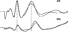
1 2 3 4
Fig. 1. Two exemples of electronically evoked auditory brainstem response (EABR) recordings in two different patients. Good intraindividual reproducibility is evident, as are the possible variations of amplitudes and latencies of waves II, III, and V.
eral morphologie criteria for ABR wave identification proposed by Picton et al.17 These criteria were adapted to the peculiarities of electrically evoked ABRs, as described in the literature: the electrically elicited response occurs approximately 2 milliseconds earlier than with acoustic stimulation. We included only reproducible waves on each of two recordings.
Statistical Analysis
The possible relationship between the behavioral threshold and the EABR threshold was examined using a parametric Pearson's correlation test (P-to-reject-correlation 0.05): the higher the r value, the better the correlation.
RESULTS
Morphology, Amplitudes, and Latencies
EABRs were able to be recorded from all the subjects. Figure 1 shows two examples of EABR in two different patients. These two examples demonstrate the good quality of the curves obtained and the good intraindividual reproducibility on test-retest evaluation (the second session being performed 6 weeks later). Wave latency and amplitude could differ across subjects. It is noteworthy that the performance of these two subi ects had changed markedly after 6 months' rehabilitation. (Open-set word recognition was 44% in patient M.B. and 22% in patient B.Ri., with CI alone, without the aid of lip reading.)
Behavioral and EABR measurements could be obtained from 55 of a total of 56 electrodes. In patient A.M., we were able to obtain neither EABR (Fig. 2) nor behavioral measures for electrode no. 10; we concluded that there was failure of this electrode.
Figure 3 shows EABR recordings in the child (patient A.M.) stimulus intensity (arbitrary device units) decreased from level 1 to level 8. These curves were reproducible for each level of stimulus current intensity; the higher the intensity, the greater the various wave amplitudes. Three peaks are well identified: the first is that of w ie II (at about 1.25 milliseconds), the second of wave III (at about 2 milliseconds), and the third of wave V (at about 3.8 milliseconds).
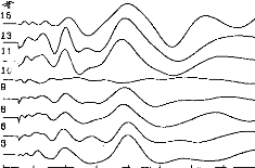
0 1 2 3 4 5 6 7 8
Fig. 2. EABR recordings in child patient. Among the eight tested electrodes, we could not obtain any response in only one case (no. 10). The stimulus artifact has been eliminated from the various recordings.
TABLE I.
Mean Latency Values and Mean Amplitude Values.
|
Means (ms) (DS) |
Amplitudes (gV) (DS) |
|||
|
Wave II |
1.28 |
(0.18) |
0.24 |
(0.10) |
|
Wave III |
2.06 |
(0.19) |
0.43 |
(0.16) |
|
Wave V |
3.90 |
(0.27) |
0.37 |
(0.13) |
Table I reports mean amplitude and latency for the various waves; the intervals between the waves are also reported.
Thresholds
Thresholds were able to be determined for all patients. Figures 4 and 5 show two examples. We looked for a possible correlation between objective threshold (determined by EABR) and subjective T-level threshold (determined by perceptual measurement). It is worth emphasizing once again the great difficulty of determining behavioral T- and C-level thresholds in pediatric patients soon after implantation. Subjective (ST) and objective (OT) threshold values were expressed in arbitrary device units, and then compared by Pearson's correlation testing. The correlation coefficient found was excellent (n = 31, r = 0.98; P < 0.001). The scatterplot illustrating this strongly positive linear relationship is presented in Figure 6. The simple regression equation (OT = 1.06 x ST + 0.22) further attests to the strength of the relationship. This also means that the objective thresholds underestimate perceptual thresholds, although the corrective factor is weak; the regression equation approximates y = X.
DISCUSSION
These results demonstrate the possibility of goodquality EABR recordings in Digisonic DX10 CI users, both adults and children.
EABR Compared With ABR
Our results agree with numerous previous published data showing earlier latencies with EABR than
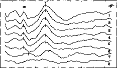
0 1 2 3 4 5 6 7 8 9 10
IChildren Threshold : Patient MOI
Fig. 3. EABR in child patient. Eight levels of stimulation are shown for electrode no. 7, decreasing from level 1 to level 8.
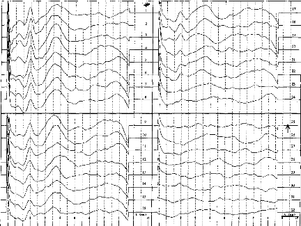
Fig. 4. EABR recordings in adult patient. Thirty-two decreasing levels of stimulation are shown for electrode no. 10. The EABR threshold is identified where waves III and V vanish simultaneously (level 25).
with ABR.18-20 This is easily explained by the direct stimulation of the acoustic nerve without delay attributable to travel through the outer and the middle ear. With acoustic stimulation in nondeaf patients, wave II is recorded with a mean 2.90-millisecond (#177;0.22) delay, wave III with a mean 3.84-millisecond (#177;0.20) delay, and wave V with a mean 5.60-millisecond (#177;0.20) delay21; other studies have reported quite similar delays: respectively, 2.92, 3.95, and 5.85 milliseconds for waves II, III, and V.22 In our experiment with EABR, wave II was observed with a mean 1.20-millisecond (#177;0.14) delay, wave III with a mean 1.89-millisecond (#177;0.20) delay, and wave V with a mean 4.09-millisecond (#177;0.26) delay. Interwave delays were identical to those recorded with acoustical stimulation in non-deaf subjects: wave II to wave III delay is 1.03 milliseconds, wave II to wave V delay is 2.81 milliseconds, and wave III to wave V delay is 1.89 mil
TABLE II.
Mean Values of Interwave Intervals.
Delays (ms)
Wave II-wave III 0.78
Wave II-wave V 2.61
Wave III-wave V 1.84
Laryngoscope 108: April 1998 Truy et al.: Cochleadments
liseconds with acoustic stimulation22 and were, respectively, recorded with 0.78-, 2.61-, and 1.84-millisecond latencies in our study. Table I presents these data.
In our patients the disappearance of waves III and V (defining objective threshold) was concomitant and without prior increase in the latencies of these waves, as mentioned. With acoustic stimulation, wave III disappears before wave V and latencies increase, with an updown procedure.
Tuning Aid Procedures
EABR can be affected by factors such as number of sweeps and subject state. The maps used in this study were obtained using standard clinical techniques with routine stimulation parameters and were the actual maps used by the subjects in their everyday rehabilitation program.
The correlations between subjective and objective thresholds were strong. The present data are the first published on Digisonic patients; other data have essentially concerned the Nucleus device.23,24 These studies reported good but not perfect correlation coefficients (r value of 0.89 in Hodges et a1.24); Shallop et al.25 found EABR thresholds to approximate C-levels, although with several instances where EABR threshold exceeded Clevel by more than 20 device units. Brown et al.10 found that the majority of EABR thresholds fell between 30%
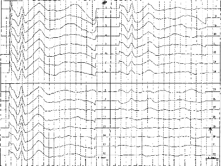
Fig. 5. EABR recordings in adult patient. Thirty-two decreasing levels of stimulation are shown for electrode no. 14. The EABR threshold is identified where waves III and V vanish simultaneously (level 29).
and 80% of dynamic range, and that only four EABR thresholds of a total of 115 exceeded C-level, and in no case by more than five device units. Mason et al.11 found EABR thresholds to exceed T-level by an average of 35 units; results reported by Brown et al.10 are consistent
0 10
Perceptual Threshold
20 30
(equipment--determined units)
ABR Th.= 0.22 + 1.06 Per.Th. N = 31
R = 0.98 P< 0.001
·· -
·!je _
·
|
|
|
||
E 35 t
'e 30
o
D-
oc
c
E. _
a
· c
*c* 20
E
o
0
co
25
15 10 5
Fig. 6. Scatterplot and linear regression equation showing the relationship between behavioral thresholds (BTs) and EABR thresholds (objective thresholds [OTs]). Symbols represent the data obtained from seven adult cochlear implant users. The continuous line is the linear regression curve, and the dotted line plots the y = x equation.
with these data. In these two studies,1°,11 it is reported that on average the difference between EABR threshold and T-level is somewhat greater for adults than for children, because T-levels found in children may be slightly above threshold. More data are needed, from a larger pediatric Digisonic-implanted population, to compare adult and pediatric EABR thresholds. We did not record any preoperative EABRs to be compared with postoperative EABRs, as reported in some studies. Mason et al.11 described preoperative EABR in children, but linear regression analysis revealed no strong correlation between preoperative EABR threshold and postoperative behavioral threshold measurements: objective threshold overestimated subjective threshold levels.
Objective threshold measurement is obviously of major importance in pediatric populations. We insist on the fact that, in the procedure described, the stimuli employed to evoke the EABRs are strictly the same as those delivered in auditory conditions during rehabilitation. This is one of the major differences with EABRs obtained through the Nucleus device'1; EABR stimulation modes described include bipolar mode (BP) +5, +10 or +20, which are very different from those of normal implant functioning (BP or BP + 1). Abbas and Brown26 reported a good correlation between subjective and objective thresholds using BP + 5 strategy in Nucleus CI users and in Ineraid CI users.
Electrode Dysfunction Diagnosis
In our sample we only obtained no artifact or EABR in the case of one electrode. This electrode dysfunction was confirmed by the absence of any signal when we used the stimulogram method, as described by other authors,27 and the average electrode voltage method.28 These two techniques are easy to perform and recordings are short, that no sedation is needed in adults or children. They can be easily employed during surgery to assess implant functioning. The average electrode voltage is a refined artifact recording method.
CONCLUSION
Different procedures are employed or assessed to evaluate the electrophysiologic responses evoked by a CI. We advocate the rapid development of objective methods in pediatric populations, which may provide useful information for tuning in children.
BIBLIOGRAPHY
1. Moore D. Postnatal development of the mammalian central auditory system and the neural consequences of auditory de- privation. Acta Otolaryngol Suppl (Stockh) 1983;421:19-30.
2. Webster DB, Webster M. Effect of neonatal conductive hearing loss on brain stem auditory nuclei. Ann Otol Rhinol Laryngol 1979;88:684-98.
3. Hall RD. Estimation of surviving spiral ganglion cells in the deaf cat using the electrically evoked auditory brainstem responses. Hear Res 1990;45:123-36.
4. Lambert PR, Ruth RA, Hodges AV. Multichannel cochlear implant and electrically evoked auditory brainstem responses in a child with labyrinthitis ossificans. Laryngoscope 1991;101:14-9.
5. Burton MJ, Miller JM, Kileny PR. Middle latency responses. Part I. Electrical and acoustic stimulation. Arch Otolaryngol Head Neck Surg 1989;115:432-457.
6. Burton MJ, Miller JM, Kileny PR. Middle latency responses; Part II. Variations among stimulation sites. Arch Otolaryngol Head Neck Surg 1989;115:458-63.
7. Truy E, Morgon A, Collet L, et al. Is round-window electrical test possible in children? Ado Otolaryngol 1993;48:114-9.
8. Jerger JF, Jenkins H, Fifer R, Mecklenburg D. Stapedius reflex to electrical stimulation in a patient with cochlear implant. Ann Otol Rhinol Laryngol 1989;95:151-7.
9. Heller JW, Sinopoli T, Fowler-Brehm N, Shallop JK. The characterization of averaged electrode voltages from the Nucleus cochlear implant. Proc Ann Int Conf IEEE 1992;13:1902-8.
10. Brown CJ, Abbas PJ, Fryauf-Bertschy H, Kelsay D, Gantz BJ. Intraoperative and postoperative electrically evoked auditory brainstem responses in nucleus cochlear implant users: implications for the fitting process. Ear Hear 1994; 15(2):168-76.
11. Mason SM, Sheppard S, Garnham CW, Lutman ME, O'Donoghue GM, Gibbin KP. Improving the relationship of intraoperative EABR thresholds to T-level in young children receiving the Nucleus cochlear implant. In:
Laryngoscope 108: April 1998
Truy et al.: Cochlear Implants
Hochmair-Desoyer IJ, Hochmair ES, eds. Advances in Cochlear Implants. Wien: Manz; 1993:44-9.
12. Allum JH, Shallop JK, Hotz M, Pfaltz CR. Characteristics of electrically evoked auditory brainstem responses elicited with the Nucleus 22-electrode intracochlear implant. Scand Audiol 1990;19:263-7.
13. Gardi JN. Human brain stem and middle latency responses to electrical stimulation: preliminary observations. In: Schindler RA, Mezernich MM, eds. Cochlear implants. New York: Raven; 1985:351-63.
14. Shallop JK, Beiter AL, Goin DW, Mischke RE. Electrically evoked auditory brainstem responses (EABR) and middle latency responses (MLR) obtained from patients with the Nucleus multichannel cochlear implant. Ear Hear 1990; 11(1):5-15.
15. Hodges AV. The relationship between electric auditory evoked responses and psychophysical percepts obtained through a Nucleus 22-channel cochlear implant. Charlottesville, VA: University of Virginia, 1990. Dissertation.
16. Gallego S, Micheyl C, Berger-Vachon C, Truy E, Morgon A, Collet L. Ipsilateral ABR with cochlear implant. Acta Otolaryngol (Stockh) 1996;116:1604-10.
17. Picton TW, Hillyard SA, Krausz HI, Gallambos R. Human auditory evoked potentials. Part I. Evaluation of components. Electroencephalogr Clin Neurophysiol 1974;36:179-190.
18. Pelizzone m, Kasper A, Montandon P. Electrically evoked responses in cochlear implant patients. Audiology 1989;28: 230-8.
19. Van Den Honert C, Stypulkowsky PH. Characterization of the electrically evoked auditory brainstem response (ABR) in cats and in humans. Hear Res 1986;21:109-26.
20. Abbas PJ, Brown CJ. Electrically evoked brainstem potentials in cochlear implant patients with multi-electrode stimulation. Hear Res 1988;36:153-62.
21. Harkins SW. Effects of age and interstimulus interval on brainstem auditory evoked potentials. Int J Neurosci 1981; 15:107-18.
22. Stockard JJ. Nonpathologic factors influencing brainstem evoked auditory potentials. Am J Electroencephalogr 1978; 18:177-209.
23. Kileny PR, Zwolan TA, Zimmerman-Phillips S, Telian SA. Electrically evoked auditory brain-stem responses in paediatric patients with cochlear implants. Arch Otolaryngol Head Neck Surg 1994;120:1083-90.
24. Hodges AV, Ruth RA, Lambert PR, Balkany TJ. Electric auditory brain-stem responses in Nucleus multichannel cochlear implant users. Arch Otolaryngol Head Neck 1994;120:1093-9.
25. Shallop JK, Van Dyke L, Goin DW, Mischke RE. Prediction of behavioral thresholds and comfort values for Nucleus 22- channel implant patients from electrical auditory brainstem response test results. Ann Otol Rhinol Laryngol 1991;100:896-8.
26. Abbas PJ, Brown CJ. Electrically evoked auditory brainstem responses: growth of response with current level. Hear Res 1991;51:123-137.
27. Almqvist B, Harris S, Jôsson KE. The stimulogram. In Hochmair-Desoyer IJ, Hochmair ES, eds. Advance in cochlear implants. Wien: Manz; 1993:33-6.
28. Shallop JK. Objective electrophysiological measures from cochlear implant patients. In Hochmair-Desoyer IJ, Hochmair ES, eds. Advances in Cochlear Implants. Wien: Manz; 1993:21-5.
Comme le montre la figure 101, une étude plus extensive portant sur 22 sujets au lieu de 9 retrouve cette corrélation.
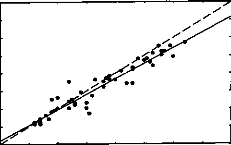
5 10 15 20 26 30 35
EABR Threahold (608
·10
Figure 101 : Relation entre le seuil de
détection subjectif à 300 Hz et le seuil d'apparition des PEAEP
à
60 Hz pour une population de 22 sujets implantés
cochléaires Digisonic.
Les études utilisant d'autres types d'implant cochléaire qui ont voulu comparer les seuils de perception (à la fréquence de stimulation du réglage) aux seuils d'apparition des PEAEP (à une fréquence plus basse) n'ont pas trouvé de fortes corrélations (Brown et al 1994, Abbas et Brown, 1991 ; Mason et al, 1994, Brown et al, 1999). Le fait que le seuil de perception à 300 Hz soit très fortement corrélé au seuil d'apparition des PEAEP (R2=0.96) sur l'implant cochléaire Digisonic est intéressant. Il est possible d'utiliser les PEAEP pour le réglage de l'implant cochléaire. Ils permettent non seulement de voir si la stimulation électrique sur une électrode provoque une réponse du système auditif mais aussi de mesurer objectivement l'intensité minimale de stimulation pour laquelle le patient aura une sensation auditive (ce qui est très difficile à obtenir chez les enfants et adultes mal conditionnés). De plus le seuil d'apparition des PEAEP est très proche du seuil de perception à 300 Hz. Cela peut s'expliquer pour plusieurs raisons. Le seuil de perception sur l'implant cochléaire Digisonic est très stable pour les fréquences comprises entre 50 et 1000 Hz (cf partie psychophysique). La technique de recueil et de traitement numérique des PEAEP permet d'obtenir des PEAEP dans des conditions extrêmes (bruit physiologique et instrumental fortement réduit). La durée du pulse est utilisée pour faire varier l'intensité de stimulation ; au seuil la synchronisation est très importante car la durée du pulse est de l'ordre de 5 à 30 ps.
PEAEP et sonie
Bien que les seuils d'inconforts diffèrent en fonction de la fréquence de stimulation, nous avons étudier les relations qu'il pourrait exister entre la fonction de sonie à 300 Hz et les caractéristiques entrée-sortie des PEAEP à 75 Hz.
S. Gallégo, S. Garnier, C. Micheyl, E. Truy, A. Morgon,
L. Collet
Acta Otolaryngol, 1999, 119, 234-238
L'objectif de cet article est de comparer la fonction de sonie aux caractéristiques des PEAEP.
Deux fréquences de stimulation sont analysées 75 et 300 Hz :
- Le 75 Hz correspond à une gamme compatible pour le recueil de PEAEP,
- Le 300 Hz correspond à la fréquence utilisée par le processeur pour coder le signal acoustique.
La mesure de la fonction de sonie est effectuée, par une technique catégorielle à 7 niveaux (très faible, faible, confortable mais faible, confortable, confortable mais fort, fort, très fort), sur une électrode apicale à deux fréquences de stimulation (75 et 300 Hz) chez 14 sujets implantés cochléaires Digisonic.
Le recueil des PEAEP s'effectue chez la même population, sur la même électrode à une fréquence de 75 Hz aux 7 niveaux de sonie calculés précédemment.
La comparaison entre les fonctions de sonie et la fonction entrée/sortie des PEAEP montre qu' :
Il est possible de déterminer très précisément le seuil de perception à 75 Hz et à 300 Hz à partir sur seuil d'apparition des PEAEP (respectivement, N=14, R2=0.9, p<0.001, N=14, R2=0.9, p<0.001),
Il est possible d'estimer le seuil d'inconfort à 300 Hz à partir de l'étude de la saturation de l'amplitude de l'onde V des PEAEP à 75 Hz,
L'amplitude de l'onde V évolue de manière linéaire du seuil de détection à 75 Hz jusqu'au seuil d'inconfort à 300 Hz.
La détermination de la fonction de sonie et plus particulièrement des seuils de détection et de confort à 300 Hz peuvent être estimer par l'analyse de l'onde V des recueils de PEAEP.
Acta Otolaryngol (Stockh) 1999; 119:
Loudness Growth Functions and EABR Characteristics in Digisonic Cochlear Implantees
S. GALLEGO
·, S. GARNIER', C. MICHEYL', E.
TRUY
·, A. MORGON2 and L. COLLET"
From the 'CNRS UPRESA 5020 Laboratory and 2ENT Department, Par. U, Ed. Herriot Hospital. Lyon and the 311,IXM Laboratory, Vallauris, France
Gallego S, Garnier S, Micheyl C, Truy E, Morgon A, Collet L. Loudness growth functions and EABR characteristics in Digisonic cochlear implantées. Acta Otolaryngol (Stockh) 1999; 119: 000-000.
Electrically evoked auditory brainstem responses (EABRs) and loudness functions were measured in 14 subjects equipped with an MXM Digisonic cochlear implant. EABRs were evoked by 75-Hz pulse trains presented on the apical electrode. Loudness functions at the same rate and at a rate more conventional for psychoacoustic measurements (300 Hz) were measured using a categorical loudness-scaling procedure. The results revealed a significant difference in the loudness functions measured at 75 and 300 Hz, loudness increasing more steeply with stimulus intensity for the latter rate. Significant correlations between EABR wave V thresholds and perceptual thresholds measured at both 75 and 300 Hi were observed. Furthermore, in 8 out of the 14 patients, EABR wave V saturated at a stimulus level corresponding precisely to the loudest bearable, i.e. "Too loud" level for the 300-Hz stimulation rate: this same level corresponded to the "Comfortable" loudness level for the 75-Hz stimulation rate. On average, an almost linear relationship was observed over the first half of the loudness range between the stimulus intensity, expressed as a pulse duration in log units, and wave V amplitude in dB. Although further investigation is required before maximum comfort levels can be predicted reliably from EABR measures in individual subjects, these results indicate new directions regarding the estimation of perceptual dynamic range limits on the basis of EABR measures in cochlear implantees. Key words: Please supply Key Words.
pect EABR amplitude growth functions to be related to loudness growth functions. However, so far, no clear relationship has been established between EABR wave characteristics and UCLs or other aspects of the loudness functions in CI subjects.
In the present study, we measured the EABR amplitude growth functions and loudness growth functions in 14 subjects implanted with an MXM Digisonic DX10 cochlear implant. In order to facilitate comparisons between electrophysiological and psychoacoustical measurements, the same stimulus rate of 75 Hz was used in the two types of measures. However, because this 75-Hz rate is not generally used in normal conditions of implant functioning, we also measured loudness functions at a 300-Hz stimulation rate, which is more generally used in speech coding strategies with the Digisonic device.
MATERIAL AND METHODS Subjects
Fourteen subjects (6 female, 8 male) aged from 25 to 65 years, implanted with the Digisonic DX10, took part in the study. They were ail profoundly deaf before implantation.
The Digisonic DX10 cochlear implant
The Digisonic DX10 is a 15-electrode transcutaneous cochlear implant (4). The device comprises an external and an internai, i.e. implanted part (Fig. 1). The external device performs an analysis of the acoustic
INTRODUCTION
An important step in cochlear implant (CI) fitting consists in the measurement of the dynamic range of hearing in electric stimulation. This dynamic range is bounded on one side by the faintest stimulus intensity that the subject can perceive, or the threshold, and on the other side by the maximum intensity that the subject can bear, which is otherwise called the uncomfortable level (UCL). These lower and upper limits of the dynamic range depend on several factors and are highly variable across subjects. Thus, measuring these levels in the cochlear implant patient whose device is to be set often is a necessary preliminary step in the fitting process.
Thresholds and UCLs can be determined using psychophysical procedures in adults. However, these subjective procedures are generally time-consuming, especially when accurate measurements are needed. Furthermore, they cannot always be used in children. Therefore, they would advantageously be replaced by objective measures.
Data in the literature indicate the existence of relationships between electrophysiological variables and perceptual thresholds in CI subjects. In particular, absolute thresholds have recently been shown to be correlated to the thresholds of electrically evoked auditory brainstem response (EABR) waves (1-3). If EABR thresholds are correlated to perceptual thresholds, one might expect EABR saturation levels to be related to UCLs. Furthermore, one might ex-
Scandinavian University Press. ISSN 0001-6489
signal, which leads to the extraction of relevant speech information. This analysis mainly involves analog-to-digital conversion of the acoustic signal at a sampling rate of 15.6 kHz and real-time FFT computation over a 128-point analysis window. The resulting spectrum is composed of 64 frequency bands, 122 Hz wide each, within a 0-7.8 kHz range. The implanted part of the device performs the decoding of the information received by the internai antenna and stimulates the electrodes. With normal insertion of the electrode array into the cochlea, the 15 electrodes are typically located 5-20 mm from the base.
For EABR recordings and psychophysical measurements, the external part of the device was replaced by a dedicated stimulation system, MXM Digistim, which was piloted from a personal computer through an opto-isolated serial port. This system allowed the control of the stimulus parameters: stimulated electrode, pulse magnitude, pulse duration, and stimulation frequency. Synchronization between the stimulation and EABR-recording systems was âchieved using an external trigger pulse produced by the Digistim.
The stimulation mode used in this study was "Common Ground", wherein only the addressed electrodes are activated, ail the other electrodes being connected to ground (5). The electric stimuli were produced by a pulse generator, which was able to deliver 0.5-3 mA. The pulses were of constant amplitude, but variable duration. Pulse durations ranged between 5-500 sus. Pulses were delivered on the apical electrode. Two stimulation rates were set: 75 and 300 Hz. The duration of the train pulse was 400 ms.
Loudness growth function measurements
Loudness growth functions were measured using a loudness scaling procedure (6). Forty different stimulation levels, equally spaced within the dynamic range, i.e. between the threshold and discomfort levels, were presented to the subjects, three times, in random order. On each presentation, the subject's task was to rate the loudness using one of the following categories: (0) Inaudible, (1) Very soft, (2) Soft, (3) Comfortable but soft, (4) Comfortable, (5) Comfortable but loud, (6) Loud, (7) Very loud, (8) Too loud. Loudness functions were obtained by computing the average stimulus intensity corresponding to each loudness category.
EABR recordings
EABR recordings were performed according to a method described in previous publications (1, 3, 7). The electrodes were positioned according to an Fpz placement plan, the ground electrode being placed on the contralateral lobe. Full-scale sensitivity was set at 200 AT. Bandwidth was 10-3,000 Hz. The number of sweeps for trace averaging was set at 2,000. The analysis window duration was 10 ms, corresponding to 1,024 points. The stimulation rate was 75 Hz. Stimulus artefacts were cancelled out using adaptive digital filtering (8). Fig. 2 shows typical EABR recordings obtained using this method.
Microphone
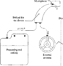
·
Behind the ear device
Skin
·
Processing and
coding
MI
Implanted electrodes
CK:_){2{:}27.C
·DC}CliCaCD*1.--i
Internai
receptor
External
antenna
Fig. I. Block diagram of the DX10 Digisonic cochlear implant. Information is transmitted from the speech processor to the internai part on a carrier wave using amplitude modulation. The carrier frequency is 4 MHz.
PIII
PV
0.2 pV
1 ms
Pll
0 1
Fig. 2. Example of. EABR recording. Waves II, III and V are iden2 3 4 5 6 7 8 tified.
tween the perceptual thresholds at there two frequencies.
An important new result obtained in the present study is that in 8 out of 14 patients, EABR wave V amplitude saturated at a stimulus level corresponding precisely to the loudness level judged as "Too loud" by the subjects with the 300-Hz stimulation rate. This "Too loud" level at 300 Hz happened to correspond to the "Comfortable" level at 75 Hz. The relationships between stimulus intensity, loudness and wave V amplitude are represented in Fig. 6, with data averaged across the 14 subjects. It can be seen on this graph that over the first half of the loudness range, i.e. over the first four loudness levels at 75 Hz, there is an almost linear relationship between wave V
RESULTS AND DISCUSSION
Loudness growth functions
Fig. 3 shows functions relating pulse widths to loudness categories. The results of a two-way repeated measures ANOVA revealed a significant effect of stimulation rate (F 30.5, p < 0.001). Pulse widths corresponding to a given loudness level were generally larger at 75 Hz than at 300 Hz. An exception to this was that at the "Very soft" loudness level, which corresponded to threshold, post hoc tests revealed no significant effect of stimulation rate.
EABRs
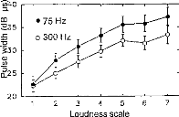
--e40
025
20
2 3 4 5 6
Loudness scale
7
Fig. 4 shows EABR wave latencies as a function of stimulus loudness. Waves II, III and V average latencies are in agreement with data from the literature (9). As can be seen on the graph, EABR latencies were not very sensitive to the loudness. The results of two-way ANOVA indicated no significant effect of the loudness level on wave III and V latencies, but a significant effect on wave II latency (F = 4.651, p < 0.001). Fig. 5 shows EABR wave amplitudes as a function of stimulus loudness. The results of a twoway repeated measures ANOVA indicated a significant effect of loudness on the amplitude of waves II (F = 5.19, p < 0.001), III (F = 6.751 p < 0.001) and V (F = 4.049 p < 0.001).
Fig. 3. Functions relating stimulus intensity and loudness at two stimulation rates (75 and 300 Hz) averaged across the 14 cochlear implantees. The correspondence between numerical loudness scores on the abscissa and verbal loudness categories is as follows: 1 Very soft, 2 = Soft, 3 = Comfortable but soft, 4 = Comfortable, 5 = Comfortable but loud, 6 = Loud, 7 = Very loud. Stimulus intensities are expressed as pulse widths in dB units, i.e. 201og10 (pulse width in ps) on the ordinate. The error bars represent the standard error of the mean.
In agreement with previous results (1-3), significant correlations were observed between EABR wave V thresholds and perceptual thresholds measured at 75 and 300 Hz (Pearson's r 0.9 p < 0.001, n= 14). This finding, that EABR thresholds correlated with perceptual thresholds measured using the same stimulus rate (75 Hz), but also a different rate (300 Hz) can be explained by the above-mentioned similarity be-
|
4.5 c; 3.0 a.) -5 2.5 o 2.0 1.5 |
2 3 4 5 6 7
Loudness scale
Fig. 4. Functions relating wave II, HI and V latencies to loudness. The scale on the abscissa is the same as in Fig. 3. Data are averaged across the 14 subjects; the error bars represent the standard error of the mean.
amplitude in dB and stimulus intensity, i.e. pulse width in log units. As can be seen on the graph, on average, the stimulus level at which wave V amplitude saturated corresponded to the "Comfortable" loudness level at 75 Hz and to the "Too loud" or uncomfortable loudness level (UCL) at 300 Hz. This relationship did not hold over the upper half of the loudness rate (beyond the "Comfortable" loudness level) due to saturation of wave V amplitude.
CONCLUSION
The present results confirm and complement previous reports indicating the existence of statistical relationships between EABR and perceptual thresholds in subjects implanted with the MXM Digisonic cochlear implant. A new element brought forward by the present study is that EABR wave V amplitude obtained at a 75-Hz stimulation rate allows the prediction of not only the absolute thresholds at this and
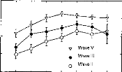
,-..., 60
cip
-a 50
a.) -a
40
E
° 30
o
e 20
2 3 4 5 6 7
Loudness scale
Fig. 5. Functions relating wave II, III and V amplitudes to loudness. The scale on the abscissa is the same as in Fig. 4. Data are averaged across the 14 subjects; the error bars represent the standard error of the mean.
Fig. 6. Relationship between stimulus intensity, loudness, and EABR wave V amplitude. The different loudness categories are represented by different symbols. The graph is based on data obtained using a 75-Hz stimulation rate, averaged across the 14 subjects; the error bars represent the standard error of the mean. The dotted lines correspond to the threshold (left) and discomfort level (right) for the 300-Hz stimulation rate.
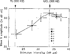
TL (300 HZ)
UCL (300 HZ)
25 30 35
Stimulus intensityy (dB 1.1.$)
40
other frequencies, but also other components of the loudness range. These include the following: the stimulus level deemed "Comfortable" by the subjects at the same low rate (75 Hz) or the "Uncomfortable" level measured with a higher rate (300 Hz), which is more conventionally used to convey information to the auditory system of cochlear implantees. Further work is certainly required before the statistical relationships between the electrophysiological and perceptual variables evidenced here can be used at the individual level for the fitting of the device.
ACKNOWLEDGMENTS
The authors acknowledge the support of the MXM Company, the ANRT, the Hospices Civils of Lyon, the CNRS, the University Lyon I, and the cochlear implantees who took part in the study.
REFERENCES
I. Gallégo S, Truy E, Morgon A, Collet L. EABRs and
surface potentials with a transcutaneous multielectrode
cochlear implant. Acta Otolaryngol (Stockh) 1997; 117:
164-8.
2. Truy E, Gallégo S, Chanal JM, Collet L, Morgon A. Correlation between electrical ABR and perceptual thresholds in Digisonic cochlear implants users. Laryngoscope 1997; 118: 554-9.
3. Gallégo S, Frachet B, Micheyl C, Truy E, Collet L. Cochlear implant performance and electrically auditory brainstem response characteristics. Electroencephalogr Clin Neurophysiol. In press.
4. Beliaeff M, Dubus P, Leveau JM, Repetto JC, Vincent P. Sound processing and stimulation coding of Digisonic DX10 15-channel cochlear implant. In: Hochmair IN, ed. Advances in cochlear implant. Innsbruck:
Verlag, 1994: 198-203.
5. Gallégo S, Ba Lê L, Berger-Vachon C. Modelling of the electrical stimulation delivered by the Digisonic Multichannel cochlear implant. Adv Model Anal 1998; 53: 1-15.
6. Jerger H, Olivier TA, Chmiel RA. Prediction of dynamic range from stapedius reflex in cochlear implanted patients. Ear Hear 1988; 9: 4-8.
7. Gallégo S, Micheyl C, Berger-Vachon C, Truy E, Morgon A, Collet L. Ipsilateral ABR with cochlear implant. Acta Otolaryngol (Stockh) 1996; 116: 228-33.
8. Gallégo S, Collet L, Berger-Vachon C. Electrically auditory brainstem responses (EABR): contribution of a
filter adapted to the auditory system. World Congress on Medical Physics and Biomedical Engineering. Nice, 14-19 September 1997. Med Biol Eng Comput 1997; 35 (Suppl 1): 304.
9. Abbas PJ, Brown CJ. Electrically evoked brainstem potentials in cochlear implant patients with multi-electrode stimulation. Hear Res 1988; 36: 53-162.
Address for correspondence:
Stéphane Gallégo
Sté MXM, 2720 chemin Saint Bernard 06227 Vallauris Cedex
France
Tel: + 33 4 93 95 18 18
Fax: + 33 4 93 95 38 01
cl PEAEP et discrimination d'intensité
La mesure du seuil différentiel en intensité est autant voir même plus important que la mesure de sonie, car elle va déterminer la résolution du codage aux différents niveaux en intensité (cf chapitre dl, enveloppe).
Des travaux chez le normo-entendant, n'ont pas pu reconstituer la fonction de sonie à partir de la mesure de discrimination en intensité car les mécanismes qui codent l'intensité de stimulation sont multiples et non linéaires.
Des mesures de la sonie et du seuil différentiel en intensité en fonction de la durée du pulse effectuées sur le Digisonic n'ont pas montré d'irrégularités, ce qui n'est pas le cas chez le normo-entendant (Raab et Taub, 1969). La détermination des IDL a partir des PEAEP chez les sujets implantés cochléaires semble donc possible.
S. Gallégo, C. Micheyl
Behavioral Neuroscience, 1998,
112, 793-799
Cet article compare la mesure du seuil différentiel en intensité (IDL) aux amplitudes et latences des PEAP pour une population normo-entendante (N=8) et une population implantée cochléaire (N=6).
Chez les sujets normo-entendants, les IDL ainsi que l'amplitude des ondes II et III varient de manière non-monotone en fonction de l'intensité de stimulation. Ces modifications non-linéaires peuvent s'expliquer par des seuils de déclenchement différents des fibres afférentes de type I au niveau de la cochlée (Liberman, 1978)
Chez les sujets implantés cochléaires, les IDL ainsi que l'amplitude des ondes II et III varient de manière monotone en fonction de l'intensité de stimulation.
L'absence de mécanismes complexes de la biomécanique cochléaire et du recrutement des fibres à différents seuils d'intensité lors d'une stimulation électrique via l'implant cochléaire Digisonic rend la fonction de IDL facilement calculable en fonction de l'amplitude des ondes.
Behavioral Neuroscience Copyright 1998 by the American Psychological Association, Inc.
1998, Vol. 112, No. 4, 793-799 0735-7044/98/$3.00
Intensity Discrimination and Auditory Brainstem Responses
in
Cochlear Implant and Normal-Hearing Listeners
Stéphane Gallégo and Christophe Micheyl
Centre National de la Recherche Scientifique
Intensity-discrimination limens (IDLs) and auditory brainstem responses (ABRs) were measured as a function of stimulus intensity in 6 cochlear implant (CI) and 8 normal-hearing (NH) listeners. Pulse-train stimuli were delivered electrically to the auditory nerve in CI listeners and acoustically in NH listeners. In CI listeners, the IDLs expressed as Weber fractions decreased monotonically with increasing intensity. In NH listeners, a nonmonotonic IDL function showing a peak a midintensities was observed. ABR wave amplitudes increased regularly with intensity only in CI listeners. Results support the notion that the slight decrease in Weber's fractions with increasing sound intensity--generally referred to as "the near-miss to Weber's law"--is subtended by retrocochlear processes, whereas the increase in Weber's fractions at midlevels--known as "the severe departure from Weber's law"--originates in cochlear mechanisms.
The encoding of intensity in the auditory system has been a matter of intense debate over the past decades, and various neurophysiological mechanisms have been put forward to account for the characteristics of auditory intensity perception evidenced by behavioral studies in animais and psychophysical measurements in humans (cf. the reviews in Phillips, 1987, and Viemeister, 1988a, 1988b). However, several basic characteristics of auditory intensity perception still lack a unequivocal neurophysiological explanation, and even the question of whether their origin is to be found at the auditory periphery or in more central parts of the auditory system remains unanswered. This is the case in particular of die so-called "near-miss to" and "severe departure from" Weber's law. The near-miss to Weber's law corresponds to the fact that intensity discrimination thresholds for pure tones, when expressed as a fraction of stimulus intensity, decrease slightly as stimulus intensity increases, whereas Weber's law would require that they remain constant (McGill & Goldberg, 1968a, 1968b; Moore & Raab, 1974). The severe departure from Weber's law corresponds to an elevation in the Weber fraction at midintensities. The severe departure was mainly studied using brief high-frequency tone bursts (Carlyon & Moore, 1984, 1986a, 1986b). However, a similar increase in Weber functions at mid intensities was originally observed using clicks (Raab &
Stéphane Gallégo and Christophe Micheyl, Unite d'Enseignement et de Recherche Associee 5020, Centre National de la Recherche Scientifique, Pavillon U Hopital E. Herriot, Lyon, France.
This work was supported by a grant from the MXM Company. We are grateful to R. P. Carlyon and R. V. Shannon for helpful comments on an earlier version of this article. L. Collet and J. D. Durrant are acknowledged for valuable comments on die results of this study. M. Rolland is acknowledged for taking part in the measurements in normal-hearing listeners.
Correspondence concerning this article should be addressed to Christophe Micheyl, UPRESA CNRS 5020, Pavillon U Hopital E. Herriot, 69003 Lyon, France. Electronic mail may be sent to cmicheyl mucosa.univ-lyon I .fr.
Taub, 1969a, 1969b). More recently, tnidlevel humps in the function relating intensity discrimination thresholds to stimulus intensity were evidenced for tones in the condition of forward masking (Zeng & Turner, 1992; Zeng, Turner, & Relkin, 1991). Whether the origin of ail these phenomena is central or peripheral, and if it is peripheral, whether it relies on cochlear mechanisms or on auditory nerve (AN) functioning, is still a matter of debate. Models based on electrophysiological recordings of AN responses indicate that only a few AN fibers with characteristic frequencies akin to that of the signal are needed to account for the intensity-discrimination performances observed in humans, but such models do not clearly account for the decrease in Weber fraction at high intensities (Viemeister, 1988a, 1988b). Regarding the existence of a midlevel hump in Weber functions, the data obtained in unmasked conditions have generally been interpreted to support a peripheral origin (Carlyon & Moore, 1984, 1986a, 1986b; Long & Cullen, 1986; Raab & Taub, 1969a, 1969b); the effects obtained in nonsimultaneous masking conditions, although originally interpreted in terras of peripheral mechanisms (Zeng & Turner, 1992; Zeng et al., 1991), are now thought to reflect more central processes (Plack & Viemeister, 1992a, 1992b).
To gain further insight into the neurophysiological mechanisms underlying the encoding of sound intensity in die auditory system, a comparison of psychophysical and physiological data is required. However, in mort cases, such a comparison is rendered difficult by the fact that the neurophysiological and the psychophysical data to be compared corne from different studies and have often been obtained using different listeners or even species. During the two preceding decades another approach to the study of the neurophysiological basis of intensity perception has become available with the development of implanted auditory prostheses delivering direct electrical stimulation to neural stages of the auditory system in humans (Shannon, 1983; Shannon & Otto, 1990). Recent studies in listeners with such auditory implants have provided important information
794 GALLÉGO AND MICHEYL
about the neurophysiological origins of perceptual phenomena relating to the perception of intensity Nelson, Schmitz, Donaldson, Viemeister, & Javel, 1996; Zeng & Shannon, 1994, 1995).
In this study, we took advantage of the two approaches currently available to investigate the neurophysiological bases of intensity perception in humans: comparisons of physiological and psychophysical measures obtained in the same listeners and comparisons of physiological and psychophysical measures between listeners with normal auditory function and listeners with an implanted auditory prosthesis. Psychophysical and physiological measures were taken from listeners with normal hearing (NH) and listeners with a cochlear implant (CI). The physiological measurements consisted of auditory brainstem responses (ABRs). The psychophysical measurements consisted of intensity-discrimination limens (IDLs) measurements. All measurements were performed at different levels spanning almost the entire audible range of the listeners. Because we wanted to make comparisons between the two kinds of measurements and the two kinds of listeners, it was important to use similar stimuli throughout the study. To minimize the differences attributable to the respective specificities of the acoustic and electrical modes of stimulation, we used stimuli with a similar temporal structure (i.e., trains of electrical or acoustic pulses presented at the same rate and having the same overall duration).
Method
Listeners
Six CI listeners (6 men, aged 28-64 years) and 8 NB listeners (5 women and 3 men, aged 20-37 years) participated in the experiment. The CI listeners were implanted with a MXM DX10 multichannel electrode device (Beliaeff, Dubus, Leveau, Repetto, & Vincent, 1994). All suffered profound bilateral sensorineural hearing loss acquired postlingually 1-8 years before implantation. In NH listeners, pure-tone audiometry was performed using a Madsen OB 822 audiometer and TDH39 earphones to ensure that auditory thresholds were not larger than 10 dB hearing loss at octave frequencies between 125 and 8000 Hz.
ABR Recordings
ABR recordings were performed using a Nicolet Pathfinder II system. The positive, negative, and reference recording electrodes were placed on the forehead, the ear lobe ipsilateral to the side of stimulation, and the contralateral ear lobe, respectively. In CI listeners, the evoking stimuli consisted of 500-ms trains of biphasic pulses. The pulses were delivered to the implant device at a rate of 60 Hz using a dedicated stimulation system (MXM Digistim). The stimulation mode was common ground. To reduce long-term stimulation fatigue and to avoid the eventual occurrence of recurrent electrical interferences, the pulse trains were separated by a silent interval of 500 #177; 100 ms. ABRs .were successively recorded at 14 stimulus levels equally spaced on a linear scale within the dynamic range (i.e., the range between the detection
threshold and the loudest bearable level in the considered CI listener). Stimulus level was controlled by varying the charge per pulse phase. Pulse amplitude remained constant; only pulse duration was varied. In each patient, the electrode with the most apical location inside the cochlea was systematically tested. For normal insertion of the electrode array into the cochlea, the location of the most apical electrode corresponded roughly to the end of the first cochlear turn. Responses were bandpass-filtered between 0.2 and 8000 Hz before being acquired at a sampling rate of 50 kHz. The averaging process involved 3,072 sweeps. Subsequent processing--adaptive filtering--was thereafter performed in die digital domain to remove stimulus artifacts. Further details about die ABR recording and processing methods may be found in previous articles (Gallégo et al., 1996; Gallégo, Truy, Morgon, & Collet, 1997). In NH listeners, ABRs were evoked using acoustic clicks. The clicks were hi-pass-filtered at a cutoff frequency of 2000 Hz. This filtering reduced trie contribution from apical generators, known to be less well synchronized than most basal generators, and at the sanie time reduced spectral cues by ensuring that successive peaks in die long-terni spectrum of the stimulus would not be resolved. The equivalent rectangular bandwidth of the auditory filter around 2000 Hz was already about four times larger than die spacing between adjacent spectral peaks corresponding to the 60-Hz click repetition rate used. As in CI listeners, the stimulus trains had a duration of 500 ms and were separated by a silent interval of 500 #177; 100 ms. The clicks were delivered in the listeners' right ear through Sony CD450 headphones. Traces at each intensity were obtained by averaging 3,000 responses. Responses were analog filtered between 100 and 1500 Hz and were then sampled at a rate of 50 kHz before further digital processing performed to cancel stimulus artifacts. ABRs were recorded at 14 stimulus intensities in 6-dB steps from 6 to 84 dB above threshold. Participants reclined in a soundproof room.
The amplitude and latency of Waves I and III were collected in NH listeners. In CI listeners, because Wave I corresponds to an electric stimulus artifact, Waves II and III were considered. Wave I in NH listeners and Wave II in CI listeners are comparable in die sense that they reflect the earliest ABR components of neural origin and are likely to originate in the activity of auditory nerve fibers.
IDL Measurements
In NH listeners, intensity discrimination limens were measured using a two-interval, two-alternative, forced-choice (2A-2IFC) procedure with a two-down/one-up adaptive rule estimating the 71% correct point on the psychometric functions. In CI listeners, a 2A-2IFC procedure combined with a method of limits was used. In both procedures, the listener's task was to indicate which of two successive intervals contained the loudest stimulus. The stimuli used for IDL measurements were the same as those used for ABRs, namely electrical biphasic pulses and acoustic clicks presented at a rate of 60 Hz in CI and NH listeners, respectively. The stimuli were 500 ms long. The interstimulus interval was 500 ms. IDL measurements were performed at levels equal to those used in ABR recordings.
Results
Intensity-Discrimination Thresholds
Figure 1 shows the average IDL function obtained from the 6 CI listeners. IDLs are expressed on the ordinate as
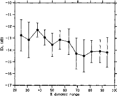
I
80
100
90
-12 -
-16-
17 t i t 1 i
20 30 40 50 60 70
% dynamic range
Figure 1. Intensity-discrimination limens (IDLs) as a function of stimulus level in cochlear implant listeners. The stimulus level is expressed as a percentage of the dynamic range on the abcissa. The mean IDLs across listeners are expressed as Weber fractions in decibels on the ordinate. The error bars represent the standard errors of the mean across listeners.
Weber fractions in decibels;' stimulus intensities are expressed on the abscissa as the percentages of dynamic range.2 The DL function could be fitted by a line with a slope of --0.03 (R2 = .73).
Figure 2 shows the average 1DL function measured in the 8 NH listeners. This function exhibited a clearly nonmono-
I I I I I I I I I I I I I 1
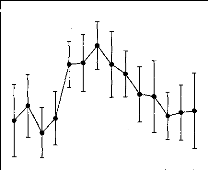
111111 I III 1111
6 12 18 24 30 36 42 48 54 60 66 72 78 84 90 Intensity (dB SL)
Figure 2. Intensity-discrimination limens (IDLs) as a function of stimulus level in normal-hearing listeners. The stimulus level is expressed in decibels SL on the abcissa. The mean IDLs across listeners are expressed as Weber fractions in decibels on the ordinate. The error bars represent the standard errors of the mean across listeners.
tonic shape characterized by a hump at intermediate stimulation levels. The statistical significance of this midlevel hump was indicated by a one-way repeated measures analysis of variance (ANOVA) performed on the data with the IDL as the dependent variable and the stimulus level as the independent variable, F(13, 91) = 2.02, p < .05. Post hoc comparisons performed using the Student's paired t test with a Bonferroni correction revealed that IDLs at 42 dB SL were significantly larger than IDLs at 18 dB SL, t(7) = 3.28, p = .013, and 72 dB SL, t (7 ) 8.06,p < .001.
Auditory Brainstem Responses
Figure 3 shows the peak amplitudes of ABR Waves II and III as a function of stimulus level in CI listeners. ABR Wave
II and Wave III amplitude increased with stimulus level. Repeated measures ANOVAs indicated a significant effect of stimulus level on ABR Wave II and Wave III amplitudes: F(50, 10) = 8.39, p < .001, for Wave II; F(50, 10) = 6.43, p < .001, for Wave III. The monotonic growth functions of the two waves could be fitted with lines (slope = 0.14, R2 = .96 for Wave II; slope = 0.23, R2 = .98 for Wave III). Figure 4 shows the latencies of Waves II and III in the CI listeners. No significant dependency of Wave II amplitude on stimulus level was observed. The latency of Wave III decreased slightly but significantly, F(50, 10) = 2.13, p < .05, as stimulus level increased.
Figure 5 shows the peak amplitudes of ABR Waves I and
III in the NH listeners. Contrary to what was observed in the CI listeners, in the NH listeners Wave I amplitude did not significantly increase with stimulus level. A significant dependency of Wave III amplitude on stimulus level was indicated by a repeated measure ANOVA, F(77, 11) = 10.81, p < .001. However, the growth function relating Wave III amplitude to stimulus level stagnated over a large range of intensities from 24 to 54 dB SL before showing a sharp increase. This was confirmed statistically using a repeated measures ANOVA, which indicated no significant differences between ABR Wave III amplitudes for stimulus intensities between 12 and 54 dB SL, no significant differ-
Various ways of expressing intensity-discrimination thresholds have been used in die literature. We used Weber fractions in decibels in this study because this metric was used in most of the studies concemed primarily with die departures from Weber's law. Furthermore, its adequacy for analyzing data from cochlear implant listeners has recently been demonstrated (Nelson, Schmitz, Donald- son, Viemeister, & Javel, 1996).
2 The specification of stimulus levels in terms of percentages of the dynamic range radier than in decibels SPL in cochlear implant listeners was motivated by results from the literature that suggest that die Weber fractions for electrical stimulation are a function of the level of the stimulus expressed in the percentage of dynamic range radier than in decibels SL (Nelson, Schmitz, Donaldson, Viemeister, & Javel, 1996).
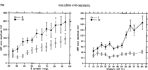
533 -
z
g 400'
w
267 -
ct
133 -
|
GALLÉGO AND MICHEYL |
|||||||||||||||||||||
|
I |
I I |
I |
I |
I |
I |
1 |
I |
I I 1 I I |
|||||||||||||
|
180 |
|||||||||||||||||||||
|
160- |
0- - - I 0- 111 |
||||||||||||||||||||
|
140- |
|||||||||||||||||||||
|
120- |
|||||||||||||||||||||
|
-o |
|||||||||||||||||||||
|
100- |
|||||||||||||||||||||
|
E |
|||||||||||||||||||||
|
w |
80- |
||||||||||||||||||||
|
60- |
|||||||||||||||||||||
|
40- |
|||||||||||||||||||||
|
20- |
|||||||||||||||||||||
|
I I |
0 |
1 |
1 1 |
I |
I |
I |
I |
I |
I |
1 1 1 1 1 |
|||||||||||
|
60 70 80 90 100 |
0 6 |
12 18 |
24 |
30 |
36 |
42 |
48 |
54 |
60 66 72 78 84 90 |
||||||||||||
Intensity (dB SL)
0
20
1 1 I
30 40 50
% dynamic range
796
800
667 -
o-11
·- - - 111
Figure 3. Auditory brainstem response (ABR) Waves II and Wave III amplitudes as a function of stimulus level in cochlear implant listeners. The stimulus levels expressed as percentages of the dynamic range on the abcissa are the same as in Figure 1. The mean amplitude of each wave across listeners is expressed in nanovolts on the ordinate. The hollow symbols correspond to Wave II. The filled symbols correspond to Wave III. The error bars represent die standard errors of die mean across listeners.
ences between ABR Wave III amplitudes for stimulus intensifies between 60 and 84 dB SL, but statistically significant differences between ABR Wave III amplitudes overall, F(11, 77) = 10.81, p < .001. Post hoc mean
Figure 5. Auditory brainstem response (ABR) Waves I and Wave III amplitudes as a function of stimulus level in normal-hearing listeners. The stimulus levels expressed in decibels SL on the abcissa are the sanie as in Figure 2. The mean amplitude of each wave across listeners is expressed in nanovolts on the ordinate. The hollow symbols correspond to Wave I. The filled symbols correspond to Wave III. The error bars represent die standard errors of die mean across listeners.
comparisons evidenced a significant difference between ABR Wave III amplitudes at 54 and 60 dB SL (Student's paired t test), t(7) = 4.94, p < .005.
Figure 6 shows the latencies of Waves I and III in die NH
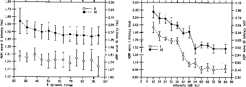
0 6 12 18 24 30 36 42 48 54 60 66 72 78 84
90
Intensif y (dB SL)
1.80
2.30
- 2.23
0- Il
1.73-
0- - - III
-2.16
-2.09
- 2.02 e, -1.95 _
1.60
20 30 40 50 60 70 80 90 100
dynamic range
7/1
I I I I I I I I I I I I I I
2.60
4.10
-3.92
-3.74
-3.56 -S
- 3.38
-3.20 .-
=
- 3.02
- 2.84 cc
co
- 2.66 -2.48
2.30
f
2.42-
Figure 4. Auditory brainstem response (ABR) Waves II and Wave III latencies as a function of stimulus level in cochlear implant listeners. The stimulus levels expressed as percentages of die dynamic range on the abcissa are die sanie as in Figures 1 and 3. Wave II mean latencies across listeners are indicated in milliseconds on the left ordinate. Wave III latencies are indicated on the right ordinate. The hollow symbols correspond to Wave II. The filled symbols correspond to Wave III. The error bars represent the standard errors of die mean across listeners.
Figure 6. Auditory brainstem response (ABR) Waves I and Wave III latencies as a function of stimulus level in normal-hearing listeners. The stimulus levels expressed in decibels SL on the abcissa are die same as in Figures 2 and 5. Wave I mean latencies across listeners are indicated in milliseconds on die left ordinate. Wave III latencies are indicated on die right ordinate. The hollow symbols correspond to Wave I. The filled symbols correspond to Wave III. The error bars represent die standard errors of the mean across listeners.
listeners. The latencies of the two waves both decreased highly significantly with increasing stimulus level: F(77, 11) = 25.02, p < .001, for Wave I; F(77, 11) = 14.75, p < .001 for Wave III.
Discussion
The main finding of this study came from the comparison of IDL functions between NH and CI listeners: Whereas in CI listeners IDL decreased overall slightly with increasing intensity, in NH listeners IDLs were found to be larger at midintensities. A second finding came from the comparison of the ABR amplitude functions between NH and CI listeners: Whereas in CI listeners the amplitude of ABR Waves II and III showed a grossly monotonie and regular dependence on stimulus level, in NH listeners ABR Waves I and III amplitudes did not significantly increase as a function of stimulus level over a large range of levels, although the latencies of the corresponding waves did significantly vary.
The observation that in CI listeners IDLs, expressed as Weber fractions, decreased when stimulus intensity was increased over the whole dynamic range is in overall agreement with results from several previous studies on intensity discrimination with electric stimulation in humans (Nelson et al., 1996; Shannon, 1983, 1992). Such a decrease in Weber fractions with increasing stimulus intensity was initially observed in NH listeners and dubbed a near-miss to Weber's law (McGill & Goldberg, 1968a, 1968b). The origin of the near-miss to Weber's law is unclear. One hypothesis is that it cornes from a broadening in the spread of excitation elicited in the peripheral auditory system as intensity is increased (Viemeister, 1983, 1988a, 1988b). In NH listeners, this level-dependent increase in the spread of excitation would occur because of nonlinear cochlear mechanisms. In CI listeners, although cochlear mechanisms are bypassed by direct electrical stimulation of the AN, some form of nonlinear spread of excitation might still occur because of spread of electrical current into the spiral ganglion (Nelson et al., 1996). In this respect, it is noteworthy that the ABR results obtained in our study, in agreement with the results from previous studies (Abbas & Brown, 1991), did not show the increase in the rate of growth of Wave II amplitude that might be expected if the rate of recruitment of AN fibers became larger at higher stimulus levels. However, because the measured peak amplitude depended not only on the number of units firing but also on the synchrony of the underlying neural events (Goldstein & Kiang, 1958), one cannot rule out the possibility that the expected increase in the rate of recruitment with increasing stimulus intensity was compensated by a lower increase in synchronization across units when more units were recruited.
A second important result of our study was the "midlevel hump" in the Weber function in NH but not in CI listeners. An increase in Weber fractions at midlevels comparable to the one observed in this study has been reported in previous studies on intensity discrimination for clicks (Avakyan & Radianova, 1963; Raab & Taub, 1969a).3 This effect,
however, failed to be replicated in a later study (Penner & Viemeister, 1973). In more recent studies, even larger increases in Weber fractions at midstimulation levels were found using short-duration, high-frequency tone bursts (Carlyon & Moore, 1984, 1986a, 1986b; Long & Cullen, 1986). Ultimately, large midlevel humps in intensity discrimination were observed with tone bursts in the condition of forward masking (Zeng et al., 1991). The origin of the increases in intensity discrimination thresholds observed in these varions studies remains unclear, and whether these effects share the same underlying mechanisms is uncertain. The psychophysical measures of IDLs obtained by Raab and Taub (1969a) were compared with recordings of the AN compound action potential in a companion study (Raab & Taub, 1969b). The results indicated that the effect was already present at the level of the AN, suggesting a peripheral origin. The studies by Carlyon and Moore (1984, 1986a, 1986b) brought forward several arguments suggesting that the midlevel hump observed with brief-duration, high-frequency tons originated at the auditory periphery. A later study of this effect further suggested that it could reflect the functioning of cochlear micromechanisms (Long & Cullen, 1986). On the contrary, the midlevel humps in intensity discrimination observed in nonsimultaneous masking conditions (Zeng & Turner, 1992; Zeng et al., 1991) were suggested to have a central origin (Plack & Viemeister, 1992a, 1992b; Zeng & Shannon, 1995). However, the relation of such effects to the effects obtained in unmasked conditions remain uncertain, and interpretations relative to their origin appear less relevant in the framework of this study. Therefore, to summarize, most, if not all, the data available in the literature on midlevel humps in unmasked conditions point to a peripheral origin.
The results of this study bring a new argument for this hypothesis. The observation of a midlevel hump in DL functions in NH listeners and the absence of this effect in CI listeners indeed suggests that the origin of this effect is to be
3 The fact that the size of the effect obtained in our study with click trains was comparable to that found in the previous study using clicks in isolation (Raab & Taub, 1969a) is noteworthy. This similarity of results suggests that the midlevel hump observed with isolated clicks was not overridden by integrative processes operating in the time domain when the stimulus was iterated. This result appears to be at variance with the hypothesis--which might be put forward to account for the fact that midlevel humps in intensitydiscrimination limens functions have generally been reported with transient or short-duration stimuli but not with longer stimuli (Carlyon & Moore, 1984)--that integrative processes operating with long-duration stimuli may compensate for the paucity of both spectral and temporal information present in short-duration stimuli, broad-bandwidth stimuli, or both. Nevertheless, the low stimulus rate used in our study leaves open the possibility that a multiple- looks mechanism, although possibly operating at higher rates, was reset from one click in the train to the other. It has been shown that clicks in a pair were integrated only when they were separated by less than about 10 ms (Viemeister & Wakefield, 1991), which is well below the 16.66-ms interval corresponding to the 60-Hz click train used in our study.
798 GALLÉGO AND MICHEYL
individual nor at the group level, this final hypothesis remains speculative.
4 The difference observed between the ranges of auditory brainstem response (ABR) wave amplitudes in cochlear implant (CI) and normal-hearing (NH) listeners may appear as a limitation to the validity of direct comparisons between the ABR growth functions obtained in the two types of listeners. However, note that the comparisons made in this study did not regard the absolute amplitude of these waves but the way they varied as a function of stimulus intensity throughout the perceptual dynamic range. The intensities used to evoke ABRs and measure Weber fractions spanned the perceptual dynamic range similarly in CI and NH listeners. The largest amplitudes obtained in CI listeners were likely to have been caused by the fact that direct electric stimulation of the AN elicited more synchronous discharges across AN fibers than acoustic stimulation (Hartmann, Topp, & Klinke, 1984; Javel, 1989; Parkins, 1989). It is not clear whether discharge synchrony across fibers is a factor of perceived intensity.
References
Abbas, P. J., & Brown, C. J. (1991). Electrically evoked auditory brainstem response: Growth of response with current level. Hearing Research, 51, 123-137.
Avakyan, R. V., & Radianova, E. A. (1963). The special features of differential intensity thresholds for a brief sound signal. Sovietic Physical Acoustics, 8, 320-323.
Beliaeff, M., Dubus, R, Leveau, J. M., Repetto, J. C., & Vincent, P. (1994). Sound signal processing and stimulation coding of the Digisonic DX10 15-channel cochlear implant. In I. J. HochmairDesoyer & E. S. Hochmair (Eds.), Advances in cochlear implants (pp. 198-203). Vienna, Austria: Manz.
Carlyon, R. R, & Moore, B. C. J. (1984). Intensity discrimination: A "severe departure" from Weber's law. Journal of the Acoustical Society ofAmerica, 76, 1369-1376.
Carlyon, R. P., & Moore, B. C. J. (1986a). Continuons versus gated pedestals and the "severe departure" from Weber's law. Journal of the Acoustical Society ofAmerica, 79, 453-460.
Carlyon, R. P., & Moore, B. C. J. (1986b). Detection of tones in noise and the "severe departure" from Weber's law. Journal of the Acoustical Society ofAmerica, 79, 461-464.
Delgutte, B. (1987). Peripheral processing of speech information: Implications from a physiological study of intensity discrimination. In M. E. H. Schouten (Ed.), Psychophysics and speech perception (pp. 333-353). Dordrecht, The Netherlands: Nijhoff.
Eggermont, J. J., & Don, M. (1980). Analysis of the click-evoked brainstem potentials in humans using high-pass noise masking: II. Effect of click intensity. Journal of the Acoustical Society of America, 68, 1671-1675.
Gallégo, S., Micheyl, C., Berger-Vachon, C., Truy, E., Morgon, A., & Collet, L. (1996). Ipsilateral ABR with cochlear implant. Acta Otolaryngologica (Stockholm), 116, 228-233.
Gallégo, S., Truy, E., Morgon, A., & Collet, L. (1997). EABRs and surface potentials with a transcutaneous multielectrode cochlear
implant. Acta Otolaryngologica (Stockholm), 117, 164-168. Goldstein, M. H. Jr., & Kiang, N. Y. S. (1958). Synchrony of neural activity in electric responses evoked by transient acoustic
stimuli. Journal of the Acoustical Society of America, 30,
107-114.
found at the level of peripheral auditory processes that are present in NH listeners and bypassed in CI listeners, namely cochlear mechanics and hair-cell transduction processes. A possible interpretation of the relationship between the worsening of intensity-discrimination performances at midintensities and the functioning of the cochlea cornes from indications that the amplitude of basilar membrane motion grows more slowly with acoustic stimulus amplitude at moderate than at low and high levels of stimulation (Robles, Ruggero, & Rich, 1986; Yates, 1990). If stimuli are discriminated in intensity on the basis of the difference in the discharge rates they evoke in auditory neurons, as suggested by several studies (Delgutte, 1987; Viemeister, 1983, 1988a, 1988b; Winslow & Sachs, 1988), the degraded intensitydiscrimination performances observed at midievels in the present and previous studies might be explainable in terms of cochlear mechanisms, as previously suggested (Long & Cullen, 1986). That would also explain that in CI listeners, cochlear mechanisms being bypassed by direct electrical stimulation of the AN, no such worsening in intensitydiscrimination performance was observed.
Another argument for a peripheral origin of the midlevel hump, which may tentatively be brought forward on the basis of the physiological results of our study, cornes from the observation of a difference between the ABR wave growth functions in NH and CI listeners. That is, whereas the amplitude of ABR Waves II and III increased regularly with stimulus level in CI listeners, in NH listeners no significant increase in the amplitude of the ABR waves was observed over a large range of moderate intensities.4 This stagnation in ABR amplitude appears to correspond to the initial saturation reported in a previous study on the dependence of ABR amplitude on stimulus level in NH listeners (Eggermont & Don, 1980). The exaggerated flatness of the growth functions shown here was attributable to the fact that near-zero ABR amplitudes at die lowest stimulus levels were not displayed and to the use of a linear y-axis scale radier than a logarithmic one, which would have expanded the rapid amplitude increase at low stimulus levels. The absence of a significant variation in ABR amplitude at moderate intensities in NH listeners could not simply be attributed to insufficient measurement sensitivity because marked variations in the latency of die same ABR waves over a corresponding range of stimulus levels were observed. Under the hypothesis that differences in stimulus intensity are encoded in the auditory system as differences in overall neural activity, reduced variations in compound neural responses should be related to reduced intensity discrimination performances. In this view, die reduced dependency of ABR amplitudes on stimulus level observed in NH listeners as compared with CI listeners may be tentatively related to the observation of reduced intensity-discrimination performance at moderate levels in these NH listeners. However, because no clear quantitative relationship between the slope of the ABR functions and the intensity discrimination thresholds could be established in our study, neither at the
Hartmann, R., Topp, G., & Klinke, R. (1984). Discharge patterns of cat primary auditory fibers with electrical stimulation of the cochlea. Hearing Research, 13, 47-62.
Javel, E. (1989). Acoustic and electrical encoding of temporal information. In J. Miller & F. A. Spelman (Eds.), Cochlear implants: Models of the electrically stimulated ear (pp. 247-
296). New York: Springer-Verlag.
Long, G. R., & Cullen, J. K. Jr. (1986). Intensity difference limens at high frequencies. Journal of the Acoustical Society ofAmerica, 78, 507-513.
McGill, W. J., & Goldberg, J. P. (1968a). A study of the near-miss involving Weber's law and pure-tone intensity discrimination.
Perception and Psychophysics, 4, 105-109.
McGill, W. J., & Goldberg, J. P. (1968b). Pure-tone intensity discrimination and energy detection. Journal of the Acoustical Society ofAmerica, 44, 576-581.
Moore, B. C. J., & Raab, D. H. (1974). Pure-tone intensity discrimination: Some experiments relating to the near-miss to
Weber's law. Journal of the Acoustical Society of America, 55,
1049-1054.
Nelson, D. A., Schmitz, J. L., Donaldson, G. S., Viemeister, N. F., & Javel, E. (1996). Intensity discrimination as a function of stimulus level with electric stimulation. Journal of the Acoustical Society of America, 100, 2393-2414.
Parkins, C. W. (1989). Temporal response patterns of AN fibers to electrical stimulation in deafened squirrel monkeys. Hearing Research, 41, 137-168.
Penner, M. J., & Viemeister, N. F. (1973). Intensity discrimination: The effects of click bandwidth and background noise. Journal of the Acoustical Society of America, 54, 1184-1188.
Phillips, D. P. (1987). Stimulus intensity and loudness recruitment: Neural correlates. Journal of the Acoustical Society of America, 82, 1-12.
Plack, C., & Viemeister, N. F. (1992a). The effects of notched noise on intensity discrimination under forward masking. Journal of the Acoustical Society of America, 92, 1902-1910.
Plack, C., & Viemeister, N. F. (1992b). Intensity discrimination under backward masking. Journal of the Acoustical Society of America, 92, 3097-3101.
Raab, D. H., & Taub, H. A. (1969a). Click-intensity discrimination with and without background masking noise. Journal of the Acoustical Society ofAmerica, 46, 965-968.
Raab, D. H., & Taub, H. A. (1969b). Fluctuations in N1 amplitude in relation to click-intensity discrimination. Journal of the Acoustical Society ofAmerica, 46, 969-978.
Robles, L., Ruggero, M. A., & Rich, N. C. (1986). Basilar
membrane mechanics at the base of the chinchilla cochlea.
Journal of the Acoustical Society of America, 80, 1364-1374.
Shannon, R. V. (1983). Multichannel electrical stimulation of the auditory nerve in man: I. Basic psychophysics. Hearing Research, 11, 157-189.
Shannon, R. V. (1992). Temporal modulation transfer function in patients with cochlear implants. Journal of the Acoustical Society of America, 91, 2156-2163.
Shannon, R. V., & Otto, S. R. (1990). Psychophysical measures from electrical stimulation of the human cochlear nucleus. Hearing Research, 47, 159-168.
Viemeister, N. F. (1983). Auditory intensity discrimination at high
frequencies in the presence of noise. Science, 221,
1206-1208.
Viemeister, N. E (1988a). Intensity coding and the dynamic
range
problem. Hearing Research, 34, 267-274.
Viemeister, N. F. (1988b). Psychophysical aspects of auditory intensity coding. In G. Edelman, W. E. Gall, & W. M. Cowan (Eds.), Auditory function (pp. 213-241). New York: Wiley.
Viemeister, N. F., & Wakefield, G. H. (1991). Temporal integration and multiple looks Journal of the Acoustical Society ofAmerica, 90, 858-865.
Winslow, R. L., & Sachs, M. B. (1988). Single-tone intensity discrimination based on AN rate responses in backgrounds of quiet, noise, and with stimulation of the crossed olivocochlear bundle. Hearing Research, 35, 165-190.
Yates, G. K. (1990). The basilar membrane input-output function. In W. L. Madison, R Dallos, C. D. Geisler, J. M. Matthews, M. A. Ruggero, & C. R. Steele (Eds.), The mechanics and biophysics of hearing (pp. 106-113). New York: SpringerVerlag.
Zeng, E-G., & Shannon, R. V. (1994). Loudness coding mechanisms inferred from electric stimulation of the human auditory system. Science, 264, 564-566.
Zeng, F.-G., & Shannon, R. V. (1995). Possible origins for the non-monotonic intensity discrimination function in forward masking. Hearing Research, 82, 216-224.
Zeng, E-G., & Turner, C. W. (1992). Intensity discrimination in forward masking. Journal of the Acoustical Society of America, 92, 782-787.
Zeng, E-G., Turner, C. W., & Relkin, E. M. (1991). Recovery from prior stimulation: H. Effects upon intensity discrimination. Hearing Research, 55, 223-230.
Received September 2, 1997 Revision received January 9, 1998 Accepted January 28, 1998
dl PEAEP et reconnaissance phonétique
Des travaux (Hermann et al, 1992 ; Gallégo et a1,1997, Groenen et al, 1997) ont montré qu'il était possible d'estimer une partie de la reconnaissance des sujets implantés cochléaires a partir de mesures électro-ph ysiolog igues.
Nous avons voulu évaluer la possible relation qu'il existe entre les PEAEP et le reconnaissance sans lecture labiale sur une population de 17 implantés cochléaires.
S. Gallégo, B. Frachet, C. Micheyl, E. Truy, L. Collet
Electroencephalography and clinical Neurophysiology, 1998, 108, 521-525
Nous avons comparé le pourcentage de reconnaissance sans lecture labiale avec les latences et intervalles des ondes II, III et V des PEAEP des 17 sujets.
Les résultats montrent de fortes corrélations entre la performance d'une part et, la latence de l'onde V (R=0.57 p=0.017), l'intervalle II-V (R=0.68 p=0.003), l'intervalle III-V (R=0.69 p=0.002) d'autre part. Nous avons ensuite modélisé ces corrélations par une fonction linéaire avec une régression linéaire multiple pas à pas. Seul l'intervalle III-V à été choisi comme modèle. La relation entre les deux paramètres est Intervalle III-V (ms) = 2.01 - 0.378 Reconnaissance (N=17 R= 0.69 p=0.002). Cette relation explique 48 % de la variance (R2).
La relation qui existe entre l'intervalle III-V et la reconnaissance de la liste de mots sans lecture labiale peut s'expliquer de la manière suivante. Un allongement anormal du temps de propagation entre l'onde III (reflétant principalement l'activité du noyau cochléaire homolatéral) et le complexe IV-V (reflétant principalement l'activité du colliculus controlatéral) se traduit par une mauvaise compréhension de la parole.
Le fait que le modèle linéaire décrivant les relations entre l'intervalle III-V et les performances des sujets porteurs de l'implant cochléaire sans lecture labiale explique environ 48 % de la variance est intéressant. La mise en place de la technique de recueil de PEAEP avant l'implantation (avec une électrode temporaire sur le promontoire ou sur la fenêtre ronde) permettrait de pouvoir estimer les performances des sujets après l'implantation.
|
ELSEVIER |
Electroencephalography and clinical Neurophysiology 108 (1998) 521-525 |
Cochlear implant performance and electrically-evoked auditory
brain-stem
response characteristics
S. Gallégo"1", B. Frachetc, C Micheyla, E. Truya'd, L. Collet"
dUPRESA--CNRS 5020, Pavillon U,
Hôpital E. Herriot, 3 place d'Arsonval, 69437 Lyon,
France
bLaboratoires MXM, 2720 chem. St Bernard, Vallauris,
France
`Service ORL, Hôpital Avicenne, Bobigny,
France
dService ORL., Pavillon U, Hôpital E. Herriot, Lyon,
France
Accepted for publication: 27 March 1998
Abstract
Objectives: The purpose of this study was to find a correlation between cochlear implant performances in phoneme discrimination and activity of the brain-stem.
Methods: Electrically-evoked auditory brain-stem responses (EABRs) and speech recognition performances were measured in 17 patients implanted with an MXM Digisonic DX10 cochlear implant. Speech recognition performances without lip-reading were tested using lists of isolated French words containing 3 phonemes.
Results: The results indicated statistically significant correlations between phoneme correct-identification scores and the following EABR variables: wave V latency, wave II-V latency interval and wave latency interval. These results, indicate that up to about 48% of the variance in isolated word recognition without lip-reading can be accounted for by EABR variables.
Conclusion: The quality of brain-stem functioning influences central processes in phoneme discrimination. (c) 1998 Elsevier Science Ireland Ltd. All rights reserved
Keywords: Cochlear implant; Electrically evoked auditory brain-stem response; Speech recognition
1. Introduction
Speech recognition performances are largely variable across cochlear implant (CI) subjects: while some patients can understand running speech in noisy backgrounds without the aid of lip-reading, others cannot recognize simple sentences spoken slowly and quietly. The speech recognition performances of a given CI subject may depend on variable factors, such as the etiology of deafness, the duration of sensory deprivation, and the language-acquisition level before implantation and motivation, and it is difficult to find a reliable predictor. The physiological state of auditory system structures appears to be an important underlying factor of overall performance with the implant. The number
* Corresponding author. UPRESA--CNRS 5020, Pavillon U, Hôpital E. Herriot, 3 place d'Arsonval, 69437 Lyon, France. Tel.: +33 4 72110530; fax: +33 4 72110504. of surviving cells in the spiral ganglion, which generaily correlates well with the duration of deafness (Otte et al., 1978; Schmidt, 1985), has been pointed out as a possible factor, not only of thresholds for electrical stimulation (Pfingst et al., 1980; Shannon, 1983; Pfingst, 1984), but also of speech recognition performances (Pauler et al., 1986) in CI subjects.
However, although results in the literature support the notion that neural survival might be reflected in the growth of electrically evoked brain-stem responses (EABRs) (Smith and Simmons, 1983; Lusted et al., 1984; Brightwell et al., 1985; Hall, 1990), the results of studies in which relationships between speech recognition performances and measures derived from EABR amplitudes, such as threshold, response growth, refractoriness and strengthduration functions have been investigated, have failed to evidence strong correlations (Abbas and Brown, 1991a,b). The results of recent studies suggest that other estimates of the neurophysiological state of peripheral and intermediate
auditory nervous structures, which are related to speech recognition performances, might be derived from late EABR wave latencies (Herman and Thornton, 1992; Gallégo et al., 1997a).
The present study sought to characterize further the relationship between speech recognition performances and EABR wave latencies in subjects implanted with the Digisonic DX10 cochlear implant.
2. Material and methods 2.1. Subjects
Seventeen adult subjects (10 female, 7 male; aged between 24 and 67 years), implanted with an MXM Digisonic DX10 cochlear implant, participated in the study. Except for the fact that a minimum of 12 out of the 15 electrodes of the implant had to be active, i.e. to elicit auditory sensations when stimulated, no particular inclusion criterion was defined regarding the etiology of deafness, the duration of deafness and the time since implantation, so as to allow for a wide range of speech recognition performances in the study sample.
2.2. The MXM Digisonic DX10 cochlear implant
The MXM Digisonic DX10 (Fig. 1) is a multi-electrode transcutaneous cochlear implant (Beliaeff et al., 1994). The implanted part of the device consists of a coil receiver and 15 0.5 mm diameter electrodes spaced 0.7 mm apart. The electrode carrier is inserted surgically along the first turn of the cochlea, generally between the 5th and the 20th mm of the basal extremity. The stimulation mode used was the `common ground' mode in which one electrode is activated at a time, all the others being connected to the ground.
Stimuli used for ABR recordings were generated using an MXM Digistim portable stimulator powered with batteries and run from a PC optically coupled to a serial port. The stimulus generator contained in this system can produce electric pulses having an intensity of up to 3 mA with a 2
load (Gallégo et al., 1998a); in the present study, the pulse amplitude was generally fixed to 1 mA. Pulse durations were varied and ranged from 5 to 310 fis. The pulses were biphasic, the positive and negative phases being asymmetric.
Each stimulation channel can be modeled as a capacitor and a resistor in series. Precise setting of the capacitor allows accurate equilibration of the positive and negative charges, which is important in order to preserve the physiological integrity of the stimulated tissues (Gallégo et al., 1998b). EABR recordings were synchronized on the stimulus using the trigger signal provided by the stimulation system.
2.3. EABR recording
An ipsilateral 3-electrode A1/2-Fpz set-up was used, with the earth electrode placed onto the contralateral ear lobe. The stimulation and recording techniques differed slightly from those used for acoustically evoked auditory brain-stem responses. The stimulation rate was 60 Hz; though such a rate would be too high for acoustically evoked auditory brain-stem responses (Suzuki et al., 1986), it has been shown to be adequate for EABRs (Gallégo and Micheyl, 1998).
The stimuli were delivered to 4 different electrodes; generally, electrode numbers 4, 7, 10 and 13. Eight stimulation levels were used; as the threshold and maximum comfort levels for electrical stimulation may vary widely across electrodes and patients, these levels were specified as percentages of the dynamic range of the tested electrode, rather

External
antenna
Skin
Implanter' electrodes
DWD
1 Internai
receiver
Behind the ear device

Microphone --\
--r

·
y

Processing and
coding
Fig. 1. Block diagram of the DX10 Digisonic cochlear implant.
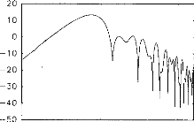
high-frequency filtering is used for the early waves whilst low-frequency filtering is used for the late waves. Fig. 2 shows the filter transfer function for the 2 ms latency wave. An algorithm for automatic wave-latency measurement based on the search for inflection points in the first derivative of the signal, combined with knowledge-based rules (Gabriel et al., 1980; Fridman et al., 1982), was then applied. Waves II, III and V latencies and the interval between waves II and III, III and V, and II and V, were considered.
2.5. Speech recognition test
To assess phonemic recognition performances, lists of 34 3-phoneme French words (`Listes cochleaires de Lafon') were used. The words recorded on CD were generated using a CD-player and presented via speakers located about 50 cm from the implant microphone. Each word was presented only once and the subject had to repeat what he/she had heard. The number of phonemes correctly identified was counted by the experimenter and expressed in percentages.
cr)
C
o
100 1000 1 000 0
Frequency (Hz)
Fig. 2. Example of digital filter transfer function used for the processing of EABR signais.
than as absolute intensities. They corresponded to 5%, 10%, 20%, 30%, 40%, 50%, 70% and 90% of the dynamic range, defined as the difference between the intensities corresponding to maximum comfort and threshold level, respectively.
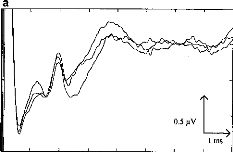
o 2 3 4 5 6 7 8
b
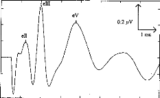
eII
o 2 3 4 5 6 7 e
Fig. 3. EABRs before (a) and after (b) digital processing. The automatic wave-latency estimation program indicated: LII = 1.22 ms, LIII = 1.98 ms, LV = 3.74 ms.
The full-scale range used for EABR recording was #177;50 p.V. Responses were filtered using a wide band (0.1-8000 Hz) analog bandpass filter. The averaging involved 1024 sweeps. In order to estimate test/re-test reproducibility, EABRs were recorded 3 times at each stimulation level. EABR reproducibility for a given stimulus intensity and electrode was calculated as the inter-correlation between 3 averages from 1 to 7 ms. EABR traces were considered reliable when the resulting inter-correlation coefficient was superior or equal to 0.15 and significant (P < 0.01); otherwise, the traces were rejected and another recording was performed.
2.4. Digital processing of EABR recordings
Following recording, the EABR traces were submitted to further analysis consisting of digital signal processing. A first problem, which is particularly acute in the case of electrically evoked ABRs, is that of the stimulus artifact, the amplitude of which can be a million-fold larger than that of the response to be measured. Therefore, special care must be taken to avoid the saturation of the pre-amplification stage. A second general problem with EABR recordings is the fact that ABR are of very small amplitude (in the sub-microvolt range), and thus generally vulnerable to interference from a variety of physical and physiological sources of noise.
Digital filters can improve greatly the ABR signal-tonoise ratio (Urbach and Pratt, 1986; Moller, 1988), with the advantage of zero phase-shift (Boston and Ainslie, 1980). In the present study, the quality of ABR traces was enhanced using an original digital-processing scheme described in a previous paper (Gallégo et al., 1997b, 1998c). This scheme is based on the use of filters with different transfer functions; for each of the ABR waves
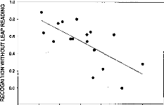
1.5 1.6 1.7 1.8 1.9 2.0 2.1 22
III-V INTERVAL (ms)
Fig. 4. Relationship between EABR wave III--V latency interval and speech-recognition scores.
3. Results 3.1. EABRs
Fig. 2 shows examples of EABR traces. The 3 upper curves (Fig. 3a) correspond to recordings prior to digital processing; the lower curve (Fig. 3b) represents the EABR after filtering and summing. Waves II, III and V can easily be identified.
3.2. Relationships between EABR variables and speech recognition performances
Using the Kolmogorov-Smirnov normality test, the wave latencies and latency intervals, averaged across electrodes and levels in each patient, were found to be normally distributed; therefore, Pearson' s parametric correlation was used to test for relationships between correct phoneme identification scores and EABR wave latencies. Significant cor- relations were found between correct phoneme recognition scores and wave V latency (r = 0.57, P < 0.05, n = 17), wave II--V latency interval (r = 0.68, P < 0.005, n = 17) and wave III--V latency interval (r = 0.69, P < 0.005, n = 17). Wave V latency and wave II--V latency interval proved to be highly correlated with wave III--V latency interval (r = 0.77 and r = 0.90, respectively; P < 0.001 and n = 17 in both cases).
Stepwise multiple regression analysis involving all EABR variables indicated wave III--V latency interval as a powerful predictor of speech recognition scores, being able to account for about 48% of the variance in the data (r = 0.69, P < 0.005, n = 17) (Fig. 4). The two variables were related by the following equation: y = 2.83 -- 1.27x, where x and y correspond to the latency interval in ms and to the speech recognition score in percentages. Another expression for the relationship between the two variables was found to be: y = 1 -- 1.27(x -- 1.44); according to this equation, the speech recognition score was 100% when the
wave III--V latency interval was as small as 1.44, and it decreased towards 0% as the interval increased up to 2.33 ms.
4. Discussion
The EABR wave latency values obtained in this study are in agreement with those available in the literature (Abbas and Brown, 1988). The variable-filter processing scheme used in the present and previous studies (Gallégo et al., 1996, 1997a) leads to clear EABR traces, allowing for accu- rate estimation of EABR wave latencies using an automatic detection algorithm.
The main result of the present study consists in a relationship between correct phoneme recognition scores on the one hand, and the latency of EABR wave V and the intervals between this latency and that of the two previous waves (II and III). The strongest predictor of speech recognition performances proved to be the wave III--V latency interval. These results generally agree with results from previous studies: in particular, Herman and Thornton (1992) evidenced a relationship between phoneme recognition performances and EABR wave V latency. More recently, Gallégo et al. (1997a) evidenced a correlation between speech recognition and wave III and V intervals.
One interpretation of the observed relationship between correct phoneme recognition percentages and EABR wave III--V latency intervals is that poor speech comprehension is connected with abnormal lengthening of the propagation time between the nervous structures that generate waves III and V. Wave III is commonly associated with the activity of the ipsilateral cochlear nucleus, while the generator of wave IV--V complex is thought to be more diffuse, involving in particular the contralateral inferior colliculus activity. A likely origin for such a lengthening in neural propagation time consists of neural degeneration. However, the fact that a relationship between EABR wave latencies and speech recognition performances was obtained specifically with wave V latency and the wave III--V latency inter- val, and not with earlier latencies or latency intervals, suggests a specific origin of the wave III--V latency interval increase. One such origin might be a reduced temporal synchrony of neural discharges at the output of the cochlear nucleus, leading to reduced temporal summation of inputs by inferior colliculus units, and consequently, increased response latencies of these units. The present results cannot be interpreted as an indication for the fact that the neurophysiological state of structures before the level of the cochlear nucleus is not an important factor of speech recognition performances in CI subjects; simply, the latencies of EABR waves associated to structures below the cochlear nucleus do not appear as a significant predictor of speech recognition performances. Because of the complexity of the neural processes involved in speech processing, relationships between electrophysiological variables and speech
recognition performances are more likely to be found at higher than at lower levels of the auditory system. Relationships between phoneme recognition performances and electrically evoked middle latency responses have recently been evidenced (Groenen et al., 1997); the results of the present study suggest that such relationships might find their origin at lower levels.
Whatever the mechanisms underlying the observed relationship between EABR wave V latency and wave III--V latency interval, the results of the present study indicate that speech recognition performances can be predicted to some extent by EABR variables. A possible application of these results might consist of pre-implantation prognostic of post- implantation speech recognition performances (Gallégo et al., 1998d). However, given that EABR characteristics appear to vary with the duration of implantation in both animais (Miller et al., 1995) and humans (Gallégo et al., 1998d), nothing yet warrants that EABR characteristics obtained using a temporary electrode installed on the promontorium or on the round window will show similar relationships with speech recognition performances.
References
Abbas, P.J. and Brown, C.J. Electrically evoked brainstem potentials in cochlear implant patients with multi-electrode stimulation. Hear. Res., 1988, 36: 153-162.
Abbas, P.J. and Brown, C.J. Electrically evoked auditory brainstem response: growth of response with current level. Hear. Res., 1991a, 51: 123-138.
Abbas, P.J. and Brown, C.J. Electrically evoked auditory brainstem response: refractory properties and strength-duration functions. Hear. Res., 1991b, 51: 139-148.
Beliaeff, M., Dubus, P., Leveau, J.M., Repetto, J.C. and Vincent, P. Sound processing and stimulation coding of Digisonic DX10 15-channel cochlear implant. In: I.N. Hochmair (Ed.), Advances in Cochlear Implant. Proceedings of the 3rd International Cochlear Implant Conference, Innsbruck, 1994, pp. 198-203.
Boston, J.R. and Ainslie, P.J. Effects of analog and digital filtering on brain stem auditory evoked potentials. Electroenceph. clin. Neurophysiol., 1980, 48: 361-364.
Brightwell, A., Rothera, M., Conway, M. and Graham, J. Evaluation of status of the auditory nerve: psychophysical test and ABR. In: R.A. Schindler and M.M. Merzenich (Eds.), Cochlear Implants. Raven, New York, 1985, pp. 343-349.
Fridman, J., John, E.R., Bergelson, M., Kaiser, J.B. and Baird, H.W. Application of digital filtering and automatic peak detection to brain stem auditory evoked potential. Electroenceph. clin. Neurophysiol., 1982, 53: 405-416.
Gabriel, S., Durrant, J.D., Dickter, A.E. and Kephart, J.E. Computer identification of waves in auditory brainstem evoked potentials. Electroenceph. clin. Neurophysiol., 1980, 49: 421-425.
Gallego, S., Micheyl, C., Berger-Vachon, C., Truy, E., Morgon, A. and Collet, L. Ipsilateral ABR with cochlear implant. Acta Otolaryngol. (Stockh.), 1996, 116: 228-233.
Gallégo, S., Truy, E., Morgon, A. and Collet, L. EABRs and surface potentials with a transcutaneous multielectrode cochlear implant. Acta Otolaryngol. (Stockh.), 1997a, 117: 164-168.
Gallégo, S., Collet, L. and Berger-Vachon, C. Electrically auditory brainstem responses (EABR): contribution of a filter adapted to the auditory system. J. Int. Fed. Med. Biol. Eng., 1997b, 35 (suppl. 1): 304.
Gallégo, S. and Micheyl, C. Relationship between auditory brainstem responses and intensity discrimination in cochlear implant patients. Behav. Neurosci., 1998 (in press).
Gallégo, S., Luu, B.L. and Berger-Vachon, C. Modelling of the electrical stimulation delivered by the Digisonic Multichannel cochlear implant. Adv. Modelling Anal., 1998a, 39(1): 39-53.
Gallégo, S., Beliaeff, M., Frachet, B., Ouayoun, M., Berger-Vachon, C. and Collet, L. Long-term change in threshold and comfort levels and dynamics in Digisonic cochlear implant bearers. 1998b (submitted).
Gallégo, S., Durrant, J., Collet, L. and Berger-Vachon, C. Numeric timevariant filters adapted to the recording of electrically evoked auditory brainstem responses (EABR). 1998c (submitted).
Gallégo, S., Truy, E., Berger-Vachon, C. and Collet, L. Electrically auditory brainstem responses in cochlear implant assessment: possibility and interest. 1998d (submitted).
Groenen, P., Snik, A. and van den Broek, P. Electrically evoked auditory middle latency responses versus perception abilities in cochlear implant users. Audiology, 1997, 36: 83-97.
Hall, R.D. Estimation of surviving spiral ganglion cells in the deaf rat using the electrically evoked auditory brainstem response. Hear. Res., 1990, 45: 123-136.
Herman, B. and Thornton, A. Electrically evoked-evoked auditory brainstem responses in cochlear implanted subjects (abstract). In: The Second International Cochlear Implant Symposium, Iowa City, IA, 1992, p. 57.
Lusted, H., Shelton, C. and Simmons, S. Comparison of electrode sites in electrical stimulation of the cochlea. Laryngoscope, 1984, 94: 878882.
Miller, C.A., Faulkner, M.J. and Pfingst, B.E. Functional responses from guinea pigs with cochlear implants. II. Changes in electrophysiological and psychophysical measures over time. Hear. Res., 1995, 92: 100-111.
Moller, A.R. Use of zero-phase digital filters to enhance brain-stem auditory evoked potentials (BAEPs). Electroenceph. clin. Neurophysiol., 1988, 71: 226-232.
Otte, J., Schuknecht, H. and Kerr, A. Ganglion cell populations in normal and pathological human cochleae. Implications for cochlear implantation. Laryngoscope, 1978, 88: 1231-1246.
Pauler, M., Schuknecht, H. and Thornton, R. Correlative studies of cochlear neuronal loss with speech discrimination and pure-tone thresholds. Arch. Otorhinolaryngol., 1986, 243: 200-206.
Pfingst, B. Operating ranges and intensity psychophysics for cochlear implants. Arch. Otolaryngol., 1984, 110: 140-144.
Pfingst, B., Telman, S. and Sutton, D. Operating ranges for cochlear implants. Ann. Otol. Rhinol. Laryngol., 1980, 89 (suppl. 66): 1-4. Schmidt, J. Cochlear neuronal populations in developmental defects of the inner ear: implications for cochlear implantation. Acta Otolaryngol. (Stockholm), 1985, 99: 14-20.
Shannon, R.V. Multichannel electrical stimulation of the auditory nerve in man. I. Basic psychophysics. Hear. Res., 1983, 11: 157-189.
Smith, L. and Simmons, F.B. Estimating eighth nerve survival by electrical stimulation. Ann. Otol. Rhinol. Laryngol., 1983, 92: 19-23.
Suzuki, T., Kobayashi, K. and Takagi, N. Effects of stimulus repetition rate on slow and fast components of auditory brainstem responses. Electroenceph. clin. Neurophysiol., 1986, 65: 150-156.
Urbach, D. and Pratt, H. Application of finite impulse response digital filters to auditory brain-stem evoked potentials. Electroenceph. clin. Neurophysiol., 1986, 64: 269-273.
Conclusion et perspectives
Les performances auditives des sujets porteurs d'un implant cochléaire présentent une grande variabilité. Les facteurs intervenant dans le succès de l'implantation sont le caractère pré- ou post- lingual de la surdité, le type de surdité, l'état de la cochlée, le nombre de fibres nerveuses survivantes, les capacités psychophysiques. La grande diversité des résultats peut également résulter de différences dans les capacités d'adaptation à la stimulation électrique, mais aussi dans les capacités cognitives des implantés.
La perception d'infimes différences auditives, essentielle pour adapter le traitement des signaux de parole, est sans doute un facteur primordial dans le succès d'une implantation cochléaire. L'utilisation de mesures électrophysiologiques qui évaluent les capacités de discrimination sont très intéressantes pour obtenir une adaptation objective de l'implant cochléaire aux capacités du sujet.
a- PEAEP
L'objectif principal des études précédentes a été d'évaluer l'intérêt des PEAEP en routine clinique pour aider au réglage de l'implant cochléaire. Il est vrai que les PEAEP ne sont pas les uniques et les plus fiables mesures électrophysiologiques qui permettent d'évaluer les caractéristiques psycho-physiques de chaque sujet implanté testé. Ils ont néanmoins l'avantage d'être fiables, robustes et rapides à obtenir.
Nous avons chercher à relier les caractéristiques des PEAEP à des seuils de détection, des seuils de confort, des discriminations en intensité et des reconnaissances phonétiques. Des études en cours, non présentés dans ce mémoire tentent de corréler des mesures de la tonie temporelle et de la tonotopie avec des recueils de PEAEP.
Les PEAEP sont des indicateurs partiels des certains paramètres tels que la tonie, l'intégration temporelle et la reconnaissance de la parole qui font intervenir des traitements plus complexes du système auditif. Les PEAEP doivent donc être couplées dans certains cas à d'autres mesures électrophysiologiques pour arriver à obtenir des estimations fiables des caractéristiques psycho- physiques.
b- PEA de latences moyennes
L'utilisation des latences moyennes a montré leur intérêt chez le normo-entendant (Bertrand et al, 1991) et chez le sujet implanté cochléaire (Polelar J et al, 1995) lorsque l'on veut mesurer la tonotopie. Certains auteurs (Groenen et al, 1997) trouvent même desrelations entre les MLR et la perception de la parole. Néanmoins ces mesures restent peu fiables et difficiles à obtenir de manière reproductible chez des sujets implantés cochléaires (Shallop et al, 1990).
c- PEA Tardifs
L'utilisation des potentiels évoqués auditifs tardifs est tout aussi possible en routine clinique que les PEAEP:
L'amplitude des ondes N1P2 est ample (plusieurs pV), reproductible et assez robuste ; le nombre de stimulation nécessaire pour avoir une courbe fiable ne dépasse pas les 100, ce qui correspond à une durée d'environ 1 min 30 s.
Des études ont montré qu'il était possible d'estimer les performances des sujets implantés cochléaires avec l'analyse des ondes tardives (ref.).
J. Wable, S. Gallégo, A.M. Jonas, I. Roussillon, E.
Truy, Y. Ormezzano, B. Frachet, L. Collet
Proceeding du Congrès de la
Société Française d'Audiologie, Clermont-Ferant,
décembre 1998
L'objectif a été d'analyser, pour une population 20 sujets implantés cochléaires Digisonic, les relations entre les caractéristiques des potentiels évoqués auditifs tardifs et les performances de reconnaissance phonétique. Contrairement à la littérature et aux PEAEP, l'étude n'a pas trouvé de liens statistiques entre la reconnaissance de la parole et les ondes de latences tardives.
Les PEAEP sont donc de meilleurs indicateurs que les PEA tardifs.
Existe-t-il une relation entre les potentiels évoqués de latence tardive et la reconnaissance de la parole chez les implantes cochléaires ?
Jocelyne Wable, Stéphane Gallégo* #, Anne-Marie Jonas, Isabelle Roussillon, Eric Truy*, Yves Ormezzano, Bruno Frachet, et Lionel Collet*.
CRISTAL, Hôpital Avicenne, Service ORL, 125 rue de Stalingrad, 93009 Bobigny, France.
* Laboratoire Perception et Mécanismes Auditifs, CNRS ESA 5020, Hôpital E. Herriot, Place d'Arsonval, 69437 Lyon.
MKM 2720 Chemin St Bernard F-06224 Vallauris Cedex, France.
Introduction
Les performances de reconnaissance de la parole sont très variables selon les sujets implantés cochléaires. Celles-ci dépendent de l'étiologie, de la durée de la surdité, de l'état du système auditif. Diverses mesures électrophysiologiques permettent d'évaluer l'intégrité du système auditif des implantés cochléaires. Les potentiels évoqués auditifs électriques de latence précoce, reflétant l'activité du tronc cérébral, ont été abondamment étudiés. De récentes études ont mis en évidence une relation entre la latence des ondes précoces et les performances (Hermann et al., 1990 ; Gallégo et al., 1998 ; Groenen et al., 1997). Les potentiels de latence tardives (N100, MMN, P300) ont reçu jusqu'à présent beaucoup moins d'attention. Ces potentiels s'avèrent intéressants dans le cadre de l'étude des processus neurophysiologiques impliqués dans la perception auditive et dans l'évaluation des dysfonctionnements (Kraus et al, 1995). Leur caractérisation chez les implantés devrait fournir un outil d'évaluation des capacités cognitives (Kraus et al., 1993).
L'objectif de notre étude est de recueillir les potentiels évoqués de latence tardive chez les implantés cochléaires pour en mesurer la latence et l'amplitude, et de confronter des données relatives à leur latence, leur amplitude avec les performances des sujets à des tests phonétiques.
Matériel et méthodes Sujets
L'étude s'est déroulée dans deux centres d'implantation. Elle concerne 20 sujets porteurs de l'implant Digisonic.
Potentiels évoqués
Les potentiels évoqués ont été évalués par stimulation de l'électrode 14 (apicale). Le stimulus consiste en une impulsion dont la durée correspond à 70 % de la dynamique du sujet. La cadence de stimulation est de 1 Hz. Les potentiels sont analysés sur une durée de 300 ms, avec un filtrage des réponses entre 1 Hz et 25 Hz. Trois enregistrements de 200 tracés sont effectués.
Tests phonétiques
La reconnaissance de la parole a été évaluée grâce à divers tests : listes de Lafon avec ou sans l'aide de la lecture labiale, avec ou sans l'implant (1 liste, 51 phonème), liste de mots monosyllabiques (10 mots), listes de phrases courtes (15 phrases), texte (durée : 5 mn)
Analyse statistique
Deux types d'analyses ont été effectuées :
· d'éventuelles corrélations entre les valeurs de latence des différentes ondes (P1, N1, P2, N2) et d'amplitude (P1N1, N1P2, P2N2) et les taux de reconnaissance (% de phonèmes reconnus ou mots/mn pour la répétition de texte) ont été recherchées.
· Les valeurs de la tence et d'amplitude des potentiels évoqués de deux groupes de patients repartis selon leurs performances ont été comparées. Pour chaque test phonétique, la population a été séparée en deux groupes en fonction des performances (50 % meilleurs,50 % moins bons).
Résultats Potentiels évoqués
Le tableau ci-dessous répertorie les différentes valeurs de latence et d'amplitude observées :
|
Latence (ms) |
Valeur |
Ecart-type |
|
P1 |
72 |
19 |
|
N1 |
105 |
19 |
|
P2 |
194 |
31 |
|
N2 |
252 |
22 |
Tests phonétiques
|
Amplitude (uV) |
Valeur |
Ecart-type |
|
P1N1 |
0.88 |
0.62 |
|
N1P2 |
1.87 |
0.98 |
|
P2N2 |
1.21 |
0.67 |
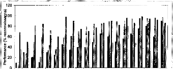
1 2 3 4 5 6 7 8 9 10 11 12 13 14 15 16 17 18 19 20
Sujets
Mots monosyllabiques ta Phrases Lafon IC Lafon IC + LL Lafon LL

Figure 1- Taux de reconnaissance des sujets aux tests
phonétiques
IC: avec implant cochléaire ; LL : avec lecture
labiale
Relation entre les potentiels évoqués et la reconnaissance de la parole
Aucune corrélation entre les taux de reconnaissance et les valeurs de latences ou d'amplitude des différentes ondes n'a été mise en évidence de manière statistique.
Lorsque les sujets sont séparés en deux groupes en fonction de leur performance, la seule différence significative est obtenue pour les latences de P2 et de N2 lorsque les sujets sont distingués en fonction de leurs performances en lecture labiale seule. Les ondes des meilleurs sujets présentent une latence plus courte (figure 2).
050 % moins bons
· 50% meilleurs
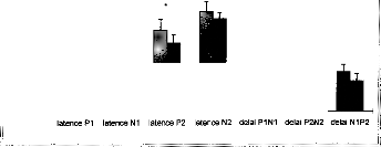

250 --
c
t 200 -- 'o
Q.
0 150 -- H
el I I I II là é I I 11111
* 100 --
I I
Lafon LL
Figure 2-
Comparaison entre les latences et intervalles
des différentes ondes de potentiels évoqués des deux
groupes de
sujets. Le test phonétique est une liste de Lafon
présentée dans la condition "lecture labiale seule". Les
deux
groupes sont bien distincts (colonnes de gauche). Les valeurs de
latences de P2 et N2 diffèrent (* p< 0.05)
Discussion
Notre étude n'a pas mis en évidence de corrélation entre les variables des potentiels évoqués tardifs et les performances de reconnaissance à la différence de Makhdoum et al. (1997). Ces auteurs observèrent une corrélation positive entre les taux de reconnaissance et les valeurs d'amplitude de l'onde N1P2, ainsi qu'une corrélation négative avec les valeurs de latence du pic P2.
En ce qui concerne les comparaisons entre les groupes de sujets distingués selon leurs performances, la seule différence de latence est obtenue dans le test de Lafon dans la condition de lecture labiale seule. Les meilleurs sujets présentent des latences plus courtes. Aucune différence relative aux amplitudes n'est observée entre les groupes. Parfois la variabilité est plus importance dans le groupes des sujets les moins bons.
Bibliographie
Gallégo S., Frachet, B., Micheyl C., Truy E., and Collet L. (1999) Cochlear implant performance and electrically evoked auditory brainstem response characteristics. EEGJ (in press).
Groenen P.A.P., Makhdoum M., Van Den Brink J.L., Stollman M.H.P., Snik A.F.M., Van Den Broek P. (1996), The relation between electric auditory brain stem and cognitive responses and speech perception in cochlear implant users. Acta Otolaryngologica, 116, 785-790.
Herman B., Thornton A. (1992) Electrically-evoked auditory brainstem responses in cochlear implanted subjects (abstr). Second International Cochlear Implant Symposium, Iowa City, IA pp 57.
Kraus N., McGee T., Carrell T., and Sharma A. (1995) Neurophysiologie bases of speech discrimination. Ear & Hearing, 16, 19-37.
Kraus N., Micco A.G., Koch D.B., McGee T., Carrell T., Sharma A., Wiet R.J., and Weingarten C.Z. (1993) The mismatch negativity cortical evoked potential elicited by speech in cochlear-implant users. Hearing Research, 65, 118-124.
Makhdoum M.J., Groenen P. AP., Snik A. FM., and van den Broek P. (1997) Intra- and interindividual correlation between auditory evoked potentials and speech perception in cochlear implant users. Scandinavian Audiology, 27, 13-20.
d- PEA Tardifs dans un protocole Rare/Fréquent
Une méthode objective utilisant les potentiels évoqués de latence tardive et permettant d'évaluer objectivement les capacités de discrimination a été développée récemment (Donchin & coll., 1978 ; Fitzgerald & Picton, 1983 ; Nââtânen & coll., 1978, 1980). Le principe de la méthode repose sur le recueil des potentiels évoqués par deux types de stimuli : l'un, dit stimulus standard, présenté de manière répétitive ; l'autre, dit stimulus déviant, présenté de manière aléatoire et rare au sein de la séquence de stimuli standards. La différence entre les potentiels évoqués par les deux types de stimuli présente une négativité aux environs de 200 ms appelée Mismatch Negativity (Nââtânen & coll., 1978, 1980) ou négativité de discordance. L'apparition de l'onde de discordance, liée à la détection automatique d'une différence, précède tout traitement linguistique du signal.
Kraus et al. (1993) ont mis en évidence l'onde de discordance lors d'une stimulation électrique chez les implantés cochléaires. En utilisant des signaux de parole synthétisée de 100 ms, /da/ et /tai ils observent une réponse similaire à celle recueillie chez des sujets normo-entendants. L'utilisation clinique de cette technique dans le domaine de l'implant permettrait d'évaluer l'intégrité du système auditif, les capacités de discrimination (Kraus & coll., 1993 ; Ponton & Don, 1995), de suivre l'évolution des capacités au cours de la rééducation des sujets (Tremblay & coll;, 1997 ; Kraus & coll., 1998).
Une utilisation clinique de l'onde de discordance nécessite tout d'abord une caractérisation de cette onde. Nous avons souhaité mettre en évidence et analyser l'onde de discordance chez les implantés lors de la stimulation de deux électrodes avec un même stimulus, ceci dans le but de comparer les ondes en fonction des paramètres expérimentaux (occurrence, position des électrodes).
J. Wable, T. van den Abbeele, S. Gallégo, B.
Frachet
Accepté dans Electroencephalography and clinical
Neurophysiology
Cette étude met en évidence un effet de la cadence de stimulation sur l'amplitude des potentiels évoqués de latence tardive avec une réponse P1N1 plus ample pour les stimuli déviants que pour les stimuli standards.
Une onde de discordance est obtenue lors de la stimulation de deux électrodes différentes, l'une de manière fréquente, l'autre de manière rare. Une négativité est observée lorsque la différence des potentiels est effectuée entre celui évoqué par le stimulus déviant et celui évoqué par le stimulus standard lorsqu'ils sont physiquement différents mais également lorsqu'ils sont physiquement identiques. Aucun effet sur la latence ou l'amplitude de la négativité en fonction de l'éloignement à l'électrode de référence n'est mis en évidence, ce qui suggère que les différentes taches présentent la même difficulté. La latence de la MMN est précoce comparée aux données de Kraus et al. (1993b), ce qui peut s'expliquer par les différences de stimulation (champ libre / stimulation directe de l'implant) ou par un traitement central moins complexe dans le cas de stimulations localisées que dans le cas de sons de parole.
Mismatch negativity: a tool for the assessment of stimuli discrimination in cochlear implant subjects.
Jocelyne Wable 1, Thierry van den Abbeele 2, Stéphane Gallégo 3, Bruno Frachet 1
Centre de Recherche et d'Ingénierie des Sciences et Techniques de l'Audition et du Langage (CRISTAL),
Université Paris 13, Hôpital Avicenne, Service ORL, 125 rue de Stalingrad, 93009 Bobigny.
2 Hôpital Robert Debré, service ORL, 48 Boulevard Serurier, 75019 Paris, France.
3 MXM 2720 Chemin St Bernard F-06224 Vallauris Cedex, France.
Correspondence:
Jocelyne Wable, CRISTAL, Hôpital Avicenne, Service ORL, 125
rue de Stalingrad, 93009 Bobigny. Tel: (33) 1 48 95 59 07, fax: (33) 1 48 95 52
02, e-mail
·
jocelyne.wable@avc.ap-hop-paris.fr
keywords: event-related electrically evoked auditory potentials, mismatch negativity, cochlear implant, electrical stimulation, discrimination, speech perception, human.
Abstract
Among cochlear implant users performance vary a lot. Cognitive abilities may be involved in this variability. The mismatch negativity should provide an index of discrimination in cochlear implantees (Kraus et al., 1993b). Our aim was to analyze MMN in cochlear implant (Digisonic) subjects to assess electrode discrimination and to study the relationship between MMN and speech performance. The mismatch was elicited by stimulating three pairs of different electrodes. Two sessions were performed with both standard and deviant stimuli reversed. Speech recognition abilities were evaluated using four speech tests. The statistics included the results of 6 subjects. They indicated that MMN may be obtained when stimulating two different electrodes. A difference occurred between standard and deviant stimuli within a session but also when the response to the deviant stimulus was compared to the response of the same stimulus in a standard condition, validating the discrimination process. MMN latency was about 140 ms, and amplitude about --2.8 i.tV. No differences were shown in respect to the electrodes spacing. No relationship between MMN and speech performance was found. The clinical application of this method might be to assess the auditory processing of electrical stimuli in congenitally deaf subjects at a preimplantation stage.
Introduction
A cochlear implant consists of an electrode array placed in the scala tympani. It delivers electrical stimulation to the remaining auditory nerve fibers of deaf patients. Non-invasive and objective tools have been developed to assess auditory nerve and central auditory system functioning before and after implantation. Auditory evoked potentials have been widely used as much for evaluating the excitability of the auditory nerve before implantation and the integrity of the implant, as for facilitating the device parameters setting (Pelizone et al., 1989; Oviatt and Kileny, 1991).
Cochlear implantation success lies on speech intelligibility and speech production abilities of the patient. Implant users vary greatly in their performance. The poorer performers could benefit from parameters setting optimization at an individual level. Differences between subjects may not be entirely explained in ternis of device, ear status or number of surviving neurons. Abilities to adapt to electrical
stimulation, discrimination of stimuli, as well as cognitive capacities may be involved. Recently, relationships were found between electrically evoked brainstem responses (EABR) and speech performances (Hermann and Thornton, 1990 ; Gallégo et al., 1998 ; Groenen et al., 1997). The ability in discriminating small acoustic differences is very important for the perception and processing of speech signais. The Mismatch Negativity (MMN) method is an objective tool that provides a measure of automatic stimuli discrimination. (Nit âtânen et al., 1978; Nââtânen and Michs 1979; Nââtânen and Picton, 1987; Sams et al., 1985). This method seems likely to be interesting in the study of neurophysiologic processes of stimulus change occurring during normal perception or in pathological situations (Kraus et ai, 1993a, 1995a). MMN should provide an index of discrimination abilities.
Kraus et al. (1993b) demonstrated that MMN may be obtained in patients with cochlear implant. With 100 ms synthesized speech stimuli /da/ and /ta/, they observed some response patterns similar to those obtained in normal-hearing subjects. Ponton and Don (1995) demonstrated that the activation of two clifferent electrode pairs along the implant array elicited an MMN response. They found, with a 1-pulse stimulation, a larger and earlier MMN response for the apical electrodes than for the basal ones. Kileny et al. (1997) investigated late and cognitive evoked potentials in children with cochlear implants. They found that for the frequency contrast, shorter and stronger P3 and MMN were associated with high sentence recognition scores. Cochlear implantees may benefit from this technique in terms of electrode functioning, auditory system integrity, discrimination abilities (Kraus et al., 1993b; Ponton and Don, 1995). Moreover, it may assess evolution of capacities along training (Tremblay et al, 1997 ; Kraus et al., 1998, 1995b).
Our aim was to put forward and analyze MMN in cochlear implant subjects to assess electrode discrimination along the implant array. The main objectives were to compare event-related auditoryevoked potentials (ERPs) waves and difference waves as a fonction of the following experimental parameters: occurrence of the stimulus and stimulated electrodes. A second objective was to study the relationship between MMN and speech perception performance.
Our experiments were performed with users of Digisonic DX10 multi-electrode cochlear implant.
Material and methods
Subjects
Eight subjects were included in the experiment, ranging in age from 40 to 71 years, having been deaf from 1 to 13 years, and having been implanted from 4 to 36 months. They were all post-lingually deafened. Details concerning etiologies, length of deafness, implant experience and stimulus parameters used in this study are displayed in Table I. All subjects wore a DIGISONIC DX 10 cochlear implant (MXM).
Digisonic DX 10 system
The DX 10 Digisonic processor signal processing consists (Beliaeff et al., 1994) in assigning to the 15 implanted electrodes 15 frequency bands ranging from 100 to 7800 Hz. The signal spectral analysis relies on a Fast Fourier Transform. Each sweep, six electrodes are stimulated, corresponding to the louder bands of the spectral analysis. The amplitude of the spectral peaks determines the amount of current delivered to the corresponding electrode, i.e., the pulse duration. The frequency bands assigned to these electrodes are spaced with a linear or a logarithmic scale. Overlapping or reassigning the frequency bands is possible. The highest pitch corresponds to the first electrode and the lowest one to the 15`h.
Event-related evoked-potentials
During measurements the subjects were seated in a comfortable chair and were asked to relax with their eyes closed, but not to go to sleep. They were instructed not to pay attention to the stimuli. Stimulation
The stimuli did not go through the implant processor but were directly delivered through a Digisonic interface, the Digistim. Stimuli were presented using a passive oddball paradigm. Attention is directed away from the acoustic stimuli with an explicit instruction to ignore all auditory stimuli. Standard (n=850) and deviant (n=150) stimuli were presented in a pseudo-random sequence with at least three standard stimuli between two deviant ones.
The mismatch was elicited by stimulating two different electrodes. Three pairs of electrodes were tested : (13, 12), (13, 10), (13, 8). In order to avoid overlapping of the MMN with the waveform
components related to the physical difference between stimuli, two sessions were performed for each pair : the first session with stimulus 1 the repetitive standard and stimulus 2 the randomly interspersed deviant one, and the contra protocol with both stimuli reversed (Ponton and Don, 1995). The order of the sessions was randomized between subjects. The order of pairs and electrodes was randomized as well.
Both stimuli were 100 ms long, with 3 ms inter-pulse duration. The stimuli interval was 1 second. Stimulus level was set at about 70 % of the dynamic range. The subjects discriminated these stimuli behaviorally. An equal level of loudness of the electrodes 13 to 8 was researched before testing at this adjusted level. At the beginning of the electrophysiological measurements it was verified that the subjects detected all stimuli and that the loudness was comfortable.
Recording
The potentials were recorded from forehead/mastoid contralateral to the implant with the ground electrode on the chin. In this work, we used only this recording position, which is known to be a good location to measure MMN. The recordings were controlled using a home-made software. The recording window included 500 ms of post-stimulus time with 250 sampang points per sweep. The responses were amplified and analog bandpass filtered on-line from 0.1 Hz to 30 Hz with a CyberAmp 320 (Axon Instruments, Foster City). Using an automatic artifact rejection algorithm, the sweeps containing activity that exceeded #177;75 jiV were excluded from subsequent averaging. ERPs from deviant and standard stimuli were averaged separately for on-line visualization of the responses. However, each ERP was also stored separately to allow off-line analysis.
Derivation of the MMN
Averaged ERPs from standard and from deviant stimuli were obtained from the recording. ERPs from standard stimuli following deviant ones were not included in the averaging. The MMN, which overlaps the N1 and P2 event-related potentials components, was measured from a difference wave obtained by subtracting the response evoked by the standard stimulus from the response evoked by the deviant stimulus. Two difference waveforms were obtained: the intra-session in which stimuli were physically different (two electrodes stimulated) and the inter-session involving physically identical stimuli presented in different contexts (randomized and rare in one session vs. repetitive and frequent in
the other one). The resulting waveforms should reflect stimulus-related activities and contextual differences for the first wave, and only contextual differences for the second one. However, the contextual difference means not only deviant vs. standard stimulation but also repetition rates and number of waveforms involved (Picton et al., 1974). A lower N1 amplitude is to be expected in the case of a standard stimulation compared to a deviant one.
Speech recognition
Four tests were administered to evaluate speech recognition abilities (Table II). For each test, the stimuli were presented in random order, at a comfortable listening level with the processor set at a normal-use setting. No lip-reading help and no feedback were provided. The VCV test assesses the ability to identify consonants. Sixteen consonants were presented through a computer with a 16-bit sound card, three Urnes each, using the vowel /a/. The subject had to choose between 16 responses presented on the computer screen. The Lafon test assesses recognition of monosyllabic words. A list contants 17 words of three phonemes. A list of 75 familiar monosyllabic words was also presented. Thirty five short sentences with 119 familiar key-words was used to assess phonetic and cognitive skills. The stimuli were presented once, in an open-set condition. The percentage of consonants, phonemes, words and keywords
recognition was evaluated, respectively.
Statistics
Statistics only concemed the 6 subjects for whom the three pair discriminations were evaluated. The P1-N1-P2 wave was identified for each evoked potential. The N1 latencies were measured at the trough. The amplitudes were evaluated based upon the difference between P1 peak and Ni trough. The MMN waves were identified in both difference waves. The MMN latencies were measured at the trough. If there were two troughs in the difference waveform, one at the Ni latency and one later, the second one was taken as the MMN (Scherg et al., 1989). The amplitudes were evaluated based upon the difference between MMN onset and MMN trough. Frequency of occurrence, session and electrode effects on latency or amplitude values were tested using ANOVAs. Moreover, the morphologies of ERP evoked by the standard and deviant stimuli were examined. Ten periods of 50 ms long were defined. In each period, the responses to standard and deviant stimuli were compared as a fonction of âme. For each electrode, for
each temporal domain, the ERPs evoked by the standard stimuli or by the deviant ones were compared using an ANOVA analysis with subjects, condition, and occurrence as factors. The factor condition represented a value of 6 dimensions (3 electrodes * 2 sessions). Correlations between MMN latency or amplitude and speech recognition were tested using a Pearson coefficient.
Results
All subjects perceived the differences between the stimuli. The data set consisted of responses from 100 to 150 deviant stimuli and from 484 to 729 standard stimuli.
Event-related evoked potential pealcs analysis
Fig 1-a shows the averaged response to the standard stimulus for a representative subject. The classic P1-N1-P2 wave is obvions, with Ni latency at about 100 ms. Fig 1-b displays the grand mean averaged responses from the stimulation of electrode 13, 12, 10 and 8 as standard stimuli.
Statistical analysis (occurrence*electrode ANOVA on repeated measures, N=6) did not show any effect of occurrence or electrode on the N1 or P2 latencies. N1 occurs around 117 ms (SD=12) and P2 around 217 ms (SD=21).
Figure 2 shows the mean P IN I amplitude (a) and the mean N1P2 amplitude (b) for the standard and deviant stimuli. As no effect of the session was found, data relative to the same electrodes were gathered between sessions. The occurrence*electrode ANOVA on repeated measures on the averaged values demonstrates an effect of occurrence (F1=19.4, p1=0.007; F2=10.7, p2=0.022) and an effect of electrode (F1=4.4, p1=0.042) with interaction (F1=5.5, p1=0.024; F2=5.4, p2=0.026) on die PiN1 and N1P2 amplitudes, respectively. The post-hoc analysis, using the Student-Newman-Keuls test shows a difference between amplitude of deviants of pairs 2 and 3 vs. pair 1. For standard stimuli no differences were found. Mean PINI amplitude equals -4.3 gV (SD 1.3), and mean N1P2 amplitude equals 4.7 (SD 1.7 p.V).
Morphology analysis
The analysis of variance with condition and occurrence as factors indicates a condition effect, above all from 100 ms to 450 ms, an occurrence effect from 100 to 300 ms with a lower value for deviant stimuli in the 100-200 ms interval and a higher value in die 200-300 ms interval, and no interaction
between the condition and the occurrence. Figure 3 displays the mean ERP gathering all condition values for the standard and deviant stimuli by 50 ms periods.
Difference waves analysis
Missing values (6/72) do not allow to performe two way ANOVA tests.
Infra-session différence
Fig 4a shows the averaged responses to the standard stimulus (stimulation of electrode 13), the averaged responses to the deviant stimulus (stimulation of electrode 12), and the difference wave for a representative subject. The MMN deflection is obvious in the response to the deviant stimulus, overlapping the N1-P2 wave.
The paired t-tests did not show any differences between sessions on MMN latency (N=16, mean=145.4 ms, SD=20.4 for the first session; mean=134.4 ms, SD=26.1 for the second session) or amplitude (N=16, mean=-3.1 SD=2.4 for the first session; mean=-2.8, SD=1.0 for the second session). However, the test power was very low. One way ANOVAs on repeated measures did not show any differences between electrodes on the latency or amplitude values. The mean MMN latency is 139 ms (SD=23). Its amplitude equals -2.911V (SD=1.8). Fig 4b displays the mean MMN infra-session difference wave (N=6) for the three pairs of electrodes.
Inter-session difference
Fig 5a shows the averaged responses to die standard stimulus
(stimulation of electrode 12), the averaged responses to the deviant stimulus
(stimulation of electrode 12), and the difference wave for a representative
subject. A negativity is obvions in this difference wave. One way ANOVAs on
repeated measures did not show any differences between electrodes on the
latency or amplitude values. The mean MMN latency of 142 ms (SD=22) and
amplitude ofs -2.8 (SD=1.4) are die same as the MMN in the
Mea-session
difference. Fig 5b displays the mean MMN intra-session difference wave (N=6)
for the three pairs of electrodes.
Speech performance
Table III reports the speech tests results. The correlation analysis did not emphasize a relationship between MivLN amplitude or latency and speech performance, regardless what the speech test was. However, the low power of the correlation test did not allow to conclude to an absence of relationship.
Discussion
The aim of the study was to characterize MMN recorded from electrical stimulation of Digisonic cochlear implant subjects. A multi-electrode implant consists of several electrodes spaced along the cochlea. By stimulating neural ganglia at more-or-less specific location through these implanted electrodes, some sensation of pitch may be restored. Activation of adjacent electrode can be discriminated behaviorally. The recording of MMN by stimulating two different electrodes may be related to the measure of frequency discrimination in normal-hearing subjects. Ponton and Don (1995), comparing responses to electrode pair stimulation in cochlear implant subjects and responses to tone burst stimulation in normal-hearing subjects, found earlier MMN waves with electrical stimulation (169 ms and 155 ms for 2 kHz and 1 kHz stimuli, respectively, vs. 114 ms and 89 ms for the basal and apical pairs, respectively) which may be explained by a more synchronized activation of neurons in the case of electrical stimulation. The stimulation of the apically located electrode pairs lead to larger responses than stimulation of the basally located electrode pairs. We found a mean MMN latency of about 140 ms for apical electrode stimulation essentially. The difference in latency with the Ponton and Don (1995) study can be due to the difference in the stimulation characteristics between the two cochlear implants: adjacent electrode pair in the Ponton and Don study, one array electrode vs. adjacent electrodes and common electrode in the Digisonic implant concerned in the present study. The latter mode of stimulation may
lead to a larger spread of current and a less synchronized activation. We found a shorter MMN latency than Kraus et al. (1993b). With 100 ms synthesized stimuli /da/ (standard) and /ta/ (deviant), they found a MMN latency of 220 ms, a duration of 121 ms, and an amplitude from onset to trough of -1.7 jtV. A similar MMN occurs when the /ta/-alone waveform was taken as standard reference. The difference between the two studies earlier and greater MMN in the present may be explained by the differences in stimuli used: phonemes in free field presentation vs. direct and localized electrode stimulation which may provide a more synchronized and replicable activation of the neurons. Indeed, stimulating bypassing
the speech processor allows precise and replicable activation of specific electrodes along the implant array. Moreover, the delay observed in case of speech discrimination may be the consequence of a longer speech processing compared to the non speech processing. The difference in MMN amplitude may also be due to the difference in the recording electrode position: FÉearlobe in the Kraus et al. (1993b) study, forehead/mastoid in this one.
Several studies showed that MMN peak latency increases as the standard deviant discrimination becomes more difficult (Sam et a1.,1985, Kakauranta et al., 1989, Scherg et al.,1989). The absence of electrode effect on MMN latency or amplitude suggests that the three tasks were as difficult, i.e., electrode 8 is not easier to discriminate from electrode 13 than electrodel2.
The evoked potentials recordings airns are also to try to predict speech recognition performance. Using the Digisonic cohlear implant, Gallégo et al. (1998) found a correlation between brainstem evoked potential wave III to wave V delay and speech recognition score (r=0.69; p<0.005) with a shorter interval linked with a higher recognition score. Groenen et al. (1997) found a relationship between phoneme recognition and middle latency responses. Makhdoum et al. (1997) demonstrated a positive correlation between cortical response (N1P2 amplitude) and speech performance in cochlear implant users, and a negative correlation with P2 latency. Kileny et al. (1997) investigated late and cognitive evoked potentials in children with cochlear implants. They studied the relationship between amplitude and latency of the cognitive response and speech recognition abilities. The latency tended to be shorter for the frequency contrast than for the loudness contrast which in turn tended to be shorter than for the speech contrast. In frequency, the discrimination showed shorter and stronger P3 and MMN that were associated with high sentence recognition scores. However, our study failed to show a relationship between latency or amplitude of MMN and speech recognition abilities. This might be due to the low power of the statistical test.
Acknowledgements
The authors wish to thank the Assistance Publique --Hôpitaux de Paris for their grant (PHRC n° 094034) and the MXM Laboratory for their fmancial support. The authors also wish to thank D. Moyse for helping with the statistics, S. Labassi for editing the manuscript, and the patients who volunteered for the experiments.
References
Beliaeff M, Dubus P, Leveau J-M, Repetto J-C, and Vincent P. Sound signal processing and stimulation coding of die Digisonic DX10 15-channel cochlear implant. In Advances in Cochlear Implants. Hochmair-Desoyer I.J. and hochmair E.S. (Eds), Manz, Wien, 1994:198-203.
Gallego S, Frachet, B, Micheyl C, Truy E, and Collet L. Cochlear implant performance and electrically evoked auditory brainstem response characteristics. Electroenceph. clin. Neurophysiol. 1998;108:521-525.
Groenen P.A.P, Makhdoum M, Van Den Brink J.L, Stollman M.H.P, Snik A.F.M, and van den Broek P. The relation between electric auditory brain stem and cognitive responses and speech perception in cochlear implant users. Acta Otolaryngol. (Stockh.), 1996;116:785-790.
Groenen P.A.P, Snik A.F.M, and van den Broek P. Electrically evoked auditory middle latency responses versus perception abilities in cochlear implant users. Audiology. 1997;36:83-97.
Herman B, and Thornton A. Electrically-evoked auditory brainstem responses in cochlear implanted subjects (abstr). Second International Cochlear Implant Symposium, Iowa City, IA 1992:57.
Kaukoranta E, Sams M, Hari R, Hâmâlâinen M, and Nââtânen R. (1989) Reactions of human auditory cortex to a change in tone duration. Hear. Res.. 1989;41:15-22.
Kileny P.R, Boerst A, and Zwolan T. Cognitive evoked potentials to speech and tonal stimuli in children with implants. Otolaryngol. Head Neck Surg. 1997;117:161-169.
Kraus N, McGee T, Micco A, Sharma A, Carrel T, and Nicot T. Mismatch negativity in school-age children to speech stimuli that are just perceptibly different. Electroenceph. clin. Neurophysiol. 1993b;88:123-130.
Kraus N, Micco A.G, Koch D.B, McGee T, Carrell T, Sharma A, Wiet R.J, and Weingarten C.Z. The mismatch negativity cortical evoked potential elicited by speech in cochlear-implant users. Hear. Res. 1993a;65:118-124.
Kraus N, McGee T, Carrell T, and Sharma A. Neurophysiologie bases of speech discrimination. Ear Hear. 1995b;16:19-37.
Kraus N, McGee T, Carrel T, King C, Tremblay K, and Nicol T. Central auditory system plasticity associated with speech discrimination training. J. Cogn. Neurosci., 1995b;7(1):25-32.
Kraus N, McGee T.J, and Koch D.B. Speech sound representation, perception, and plasticity : a neurophysiologie perspective. Audiology Neuro-Otology. 1998;3:168-182.
Makhdoum M.J, Groenen P. AP, Snik A. FM, and van den Broek P. Infra- and interindividual correlation between auditory evoked potentials and speech perception in cochlear implant users. Scand. Audiol. 1997;27:13-20.
Nââtânen R, Gaillard A.W.K, and Mântysalo S. Early selective attention effect on evoked potential reinterpreted. Acta Psychologica. 1978;42:313-329.
Nââtânen R., and Michie P.T. Early selective attention effects on the evoked potential. A critical review and reinterpretation. Biol. Psychol. 1979;8:81-136.
Nââtânen R., and Picton T. The NI wave of the human electric and magnetic response to sound : a review and an analysis of the component structure. Psychophysiology. 1987;24:375-425.
Oviatt D. and Kileny P. Auditory event-related potentials elicited from cochlear implant recipients and hearing subjects. Am. J. Audiol. 1991;1:48-55.
Pelizzone M, Kasper A, and Montandon P. Electrically evoked responses in cochlear implant patients. Audiology, 1989;28:230-238.
Picton T.W., Hillyard S.A., and Krausz HI., and Galambos R. Human auditory evoked potentials. I: evaluation of components. Electroenceph. clin. Neurophysiol. 1974;36:179-190.
Ponton C. W, and Don M The mismatch negativity in cochlear implant users. Ear Hear. 1995;16:131-146.
Sams M, Hâmâlâinen M, Antervo A, Kaukoranta E, Reinikainen K, and Han R. Cerebral neuromagnetic responses evoked by short auditory stimuli. Electroenceph. clin. Neurophysiol., 1985;61:254-266.
Scherg M, Vajsar J, and Picton T.W. A source analysis of the late human auditory evoked potentials. J.Cogn. Neurosci. 1989;1:336-355.
Tremblay K, Kraus N, Carrell T.D, and McGee T. Central auditory system plasticity : generalization to novel stimuli following training. J. Acoust. Soc. Am. 1997;102:3762-3773.
Table I- Age, etiology, deprivation duration, implantation duration and electrode tested for the subjects evaluated. Pulse duration were set to deliver stimuli at about 70% of the dynamic range.
|
Subject |
Age |
Etiology |
Total deaf duration (yr) |
Implantation |
Electrode pairs tested |
|
JL |
59 |
otosclerosis |
4 |
8 |
13:33, 12:35, 10:31, 8:26 |
|
AN |
40 |
meningitis |
6 |
4 |
13:64, 12:66, 10:68, 8:68 |
|
HB |
69 |
chronic otitis |
2 |
21 |
13:22, 12:26, 10:29, 8:36 |
|
SO |
71 |
otosclerosis |
1 |
8 |
13:31,10:44, 8:38 |
|
MI |
55 |
sudden deafness |
1 |
6 |
13:16, 12:18, 10:18, 8:16 |
|
AZ |
53 |
sudden, meningitis |
7 |
12 |
13::14, 12:14, 10:16, 8:18 |
|
-SP |
65 |
sudden deafness |
13 |
28 |
13:24, 12:28 |
|
AC |
59 |
progressive deafness |
3 |
14 |
13:23, 12:25, 10:24, 8:27 |
Table II- Characteristics and evaluation criterion of speech tests.
Test Characteristics level of evaluation
VCV 16 consonants, 3 times each consonant /48
Lafon 17 monosyllabic words of three phonemes /51
phonemes
words 75 familiar monosyllabic words words /75
sentences 35 sentences, 119 key words key words /119
Table III- Speech test performance for the six subjects included in the statistical analysis.
|
Subject |
VCV |
Words |
Sentences |
Lafon IC |
||
|
ac |
42 |
57 |
80 |
82 |
||
|
an |
27 |
20 |
21 |
50 |
||
|
az |
48 |
45 |
58 |
63 |
||
|
hb |
65 |
41 |
81 |
75 |
||
|
il |
46 |
49 |
84 |
45 |
||
|
mi |
42 |
11 |
21 |
59 |
||
|
S cl) p 15. â |
||||||
0 100 200 300
Time (ms)
Figure 1-a
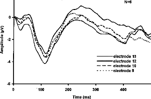
0
100
400
200 300
Time (ms)
2
electrode 13 electrode 12
-- -- -- electrode 10 electrode 8
N=6
Figure 1-b
|
pair 1 pair 2 pair 3
Electrode pairs
Figure 2a
|
standard |
pair 1 pair 2 pair 3
Electrode pairs
Figure 2b
4
2
·
·
·
n
·
·n
-4-
·** * * * ** * * * * * *
n standard
· devient
|
hO |
hO 00
|
e b' |
Time intervals (ms)
Figure 3
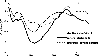
0
100
200
300
2-
li
standard : electrode 13 deviant : electrode 12 difference : deviant-standard
Time (ms)
Figure 4-a
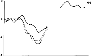

.--
...
r \
/ ...
i .p.egrfe.*1
r .s.
·
·
·
i ,
·e.
· IN
i ...%
I ;
· :114.: `
*
·
0
·
·
1,..;
deviant 12 - standard 13 -- -- -- deviant 10 - standard 13 deviant 8 - standard 13
0 100 200 300
Time (ms)
Figure 4-b

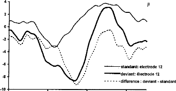
-standard: electrode 12 deviant: électrode 12 difference : deviant - standard
0 100 200 300
Time (ms)
Figure 5-a
4
deviant 12 - standard 12 -- -- -- deviant 10 - standard 10
deviant 8 - standard 8
|
2 |
I
/ % ` e -.5
..
· N
f"
·
·
·
·
· ,...,
%...'"«....
·r..,
i .."0 '
....s s. ''. 1. _.. /--«y
I . . ,.. .
.-------,s\ I ,' ...
·
·...
. ` / .....
. \
.. .".
·... / :
N=6
.. ...... .
|
100 200 300 Time (ms) |
||
|
0 |
||
Figure 5-b
Legend of figures
Figure 1- a- Averaged response of the standard stimulus for a representative subject. The classic PI-NI - P2 wave is obvions, with N1 at about 100 ms. b- grand mean averaged responses from stimulation of electrode 13, 12, 10 and 8 as standard stimuli.
Figure 2- Mean P1N1 amplitude (a) and mean N1P2 amplitude (b) for standard and deviant stimuli in respect to electrode pairs.
Figure 3- Mean ERP values for standard and deviant stimuli by 50 ms periods. The stars indicate the signification level of the comparison for each interval. *: p<0.05, **: p<0.01, ***: p<0.001.
Figure 4-a- Averaged responses of the stimulation of electrode 12 as standard stimulus, as deviant stimulus, and difference wave for a representative subject. The MMN deflection is obvions in the response of the deviant stimulus, overlapping the N1-P2 wave. b- Grand mean MMN intra-session difference wave (N=6) for the three pairs of electrodes.
Figure 5-a- Averaged responses of the standard stimulus (stimulation of electrode 12), of the deviant stimulus (stimulation of electrode 12), and difference wave for a representative subject. A negativity is obvions in this difference wave. b- Mean MMN nitra-session difference wave (N=6) for the three pairs of electrodes.
Références
Abbas PJ, Brown CJ. Electrically evoked auditory brainstem response: Growth of the response with current level. Hear Res 1991a 51:123-137
Abbas PJ, Brown CJ. Electrically evoked auditory brainstem response: Refractory properties and strength duration fonctions. Hear Res1991b 51:138-148.
Abbas PJ, Brown CJ. Electrically evoked brainstem potentials in cochlear implant patients with multi-electrode stimulation. Hear Res 1988 36:153-162
Allen JB, Hall JL, Jeng PS. Loudness grwth in 1/2 octave bands (LGOB) a procedure for the assessment of loudness. J Acous Soc Am 1990, 88 745-753
Beliaeff M, Dubus P, Leveau JM, Repetto JC, Vincent P. Sound processing and stimulation coding of Digisonic DX10 15-channel cochlear implant. Hochmair IN, ed. Advances in cochlear implant. Innsbruck: Verlag. 1994 198-203
Berger-Vachon C., Gallégo S., A. Morgon, Truy E.. Analytical Importance of the coding features for the discrimination of wovels in the cochlear implant signal. An Otol Rhinol Laryngol (1995), sup.166,104,9,2, 351353
Berger-Vachon C., Gallégo S., J.C. Bera, E. Arnoux, C. Kissac. A model of vowel representation using a cochlear implant. Proc. Inter. AMSE Symposium. Regio Calabria, (Italie), Sept 11-13 1997
Bertrand O, Perrin O, Pernier J. Evidence for a tonotopic organization of the auditory cortex observed with auditory evoked potential. Acta Otolaryngol (Sotckh) 1991, 491 116-123
Blamey PJ, Dooley GJ, Parisi ESP, Clark GM. Pitch comparison of acoustically and electrically evoked auditory sensation. Hear Res, 1996, 99 139-150
Bregman AS, Levitan R, Liao C. Fusion of auditory components. Effects of frequency of amplitude modulation. Perception and Psychophysics, 1990, 47, 68-73
Brightwell A, Rothera M, Conway M, Graham J. Evaluation of status of the auditory nerve: psychophysical test and
ABR. Eds RA Schindler & MM Merzenich Cochlear Implants Raven Press New York 1985 343-9
Brimacombe JA, Eisenberg LS. Tone decay in subjects with the single channel cochlear implant. Audiology 1984,
23 321-332
Brown CJ, Hughes ML, Lopez SM, Abbas PJ. Relationship between EABR thresholds and levels used to program the Clarion speech processor. Ann Otol Rhinol Laryngol, 1999, 108 50-57
Brown JB, Abbas PJ, Fryauf-Bertschy H, Kelsay D, Gantz BJ. Intraoperative and Postoperative Electrically Evoked Auditory Brain Stem Responses in Nucleus Cochlear Implant Users: Implications for the Fitting Process. Ear Hear 1994 15:168-176
Busby PA, Clark GM. Electrode discrimination by early-deafened cochlear implant patients. Audiology 1996 35:8- 22
Calliope. La parole et son traitement automatique. Ed Masson, 1989
Cazal Y, Pelizzone M, Kasper A, Montandon M. Indication of a relation between speech perception and temporal resolution for cochlear implantees. Ann Otol Rhinol Laryngol 1991 100:893-895
Cazal Y, Pelizzone M, Saudan O, Boex C. Amplitude modulation transfer fonctions associated with speech recognition for Ineraid cochlear implantees. Hochmair IN, ed. Advances in cochlear implant. Innsbruck: Verlag. 1994 321-325
Clark G, Shepherd R, Franz B, Dowell R, Tong Y et al. The histopathology of the human temporal bone and auditory central nervous system following cochlear implantation in patient. Acta Otolaryngol (Stockh) 1988 (suppl 448):165
Clark GM, Tong YC, Martin LFA. A multiple-charnel cochlear implant: an evaluation using closed-set spondaic words. J Laryngol 1981 95:461-464
Cohen LT, Busby PA, Whitford LA, Clark GM. Cochlear implant place psychophysics. Audiol Neurootol 1996, 1 265-277
de Sauvage RC, da Costa DL, Erre JP, Aran JM. Electrical and physiological changes during short-terni and chronic electrical stimulation of the normal cochlea. Hea Res 1997, 110 119-134
Deguine O. Implants cochléaires. Acquisition et controverses. Thèse de médecine, 1990
Dobie RA, Kimm J Brainstem responses to electrical stimulation of the cochlea. Arch Otolaryngol 1980, 106 573577
Don M, Eggermont JJ. Analyses of click-evoked brainstem potentials in man using high-pass noise masking. J Acoust Soc Am 1978 63(4):1084-1098
Donchin E., Ritter W., & McCallum C.W. (1978). Cognitive Psychophysiology : the endogenous components of the ERP. In E. Callaway, P.
Dorman MF, Loizou PC, Fitzke J, Tu Z. The recognition of sentences in noise by normal-hearing listeners using
simulations of cochlear implant signal processors with 6-20
channels. J Ascous Soc Am 1998, 104 3583-3585
Dorman MF, Smith M, Smith L,
Parkin JL. The pitch of electrically presented sinusoids. J Acous Soc Am
1994
95(3): 1677-1679
Doumèche P. L'accès au lexique chez le sujet porteur d'un implant cochléaire. Mémoire d'orthophonie, Paris, 1997 Dynes SBC, Delgutte B. Phase-locking of auditory-nerve discharges to sinusoïdal electrical stimulation of the cochlea. Hear Res 1992, 58 79-90
Eddington DK. Speech discrimination in deaf subjects with cochlear implants. J Acoust Soc Ain 1980 51:885-891 Eggermont JJ. Peripheral auditory adaptation and fatigue : a model oriented review. Hear Res 1985, 18 57-71
Fifer RC, Novak MA. Myogenic Influences on the Electrical Auditory Brainstem Response (EABR) in Humans.
Laryngoscope 1990 100:1180-1184
Fitzgerald P. and Picton T.W. (1983) Event-related potentials recorded during the discrimination of improbable stimuli. Biological Psychology, 17, 241-276.
Friesen LM, Shannon RV, Slattery WH. Speech recognition in noise as fonction of the number of electrodes used in the speak, SAS and CIS speech processors. Confrence on Implantable Auditory Prostheses, Asilomar, August 29 -- September 3, 1999.
Frijns JHM, Snoo SL, ten Kate JH. Spatial selectivity in a rotationally symmetric model of the electrically stimulated cochlea. Hear Res 1996, 95 33-48
Fu QJ, Shannon RV. Effects of amplitude nonlinearity on phoneme recognition by cochlear implant users and normal-hearing listeners. J Ascous Soc Am 1998, 104 2570-2577
Gallégo S. Préservation de l'enveloppe temporelle pour la compression du signal de parole. IVe C F Audiologie 7-8 décembre 1998, Clermont-Ferrand. Sous- presse
Gallégo S. Utilisation de la psycho-acoustique pour le réglage de l'implant cochléaire Digisonic. Conférencié invité au IVe C F Audiologie 7-8 décembre 1998, Clermont-Ferrand. Sous-presse
Gallégo S., B Frachet, Truy E., L Collet. Modification des seuils en fonction des caractéristiques du patient implanté cochléaire. IVe C F Audiologie 7-8 décembre 1998, Clermont-Ferrand. Sous-presse
Gallégo S., B. Frachet, Truy E., Collet L.. Cochlear implant performance and electrically auditory brainstem response characteristics. Electroencephalography & clin neurophysiol. (1998), 108:521-525
Gallégo S., Ba Lê Luu, Berger-Vachon C.. Modelling of the electrical stimulation delivered by the Digisonic Multichannel cochlear implant. AMSE (1998), 39, 1, 39-54
Gallégo S., C. Micheyl, Berger-Vachon C., Truy E., A. Morgon, Collet L.. Ipsilateral ABR with cochlear implant. Acta Oto-Laryngologica. (Stockholm) (1996), 116, 228-233
Gallégo S., C. Micheyl. Intensity discrimination and auditory brainstem responses in cochlear implant and normalhearing subjects. Behaviorial Neuroscience (1998), 112, 4, 793-799
Gallégo S., Collet L., Berger-Vachon C.. A model of electrical stimulation delivered by the Digisonic cochlear implant. World Congress on Medical Physics and Biomedical Engineering, Nice, 14-19 september, 1997. J Int Federation for Medical & Biological Engineering, 35 (suppl), 1, 300
Gallégo S., Collet L., Berger-Vachon C.. Electrically auditory brainstem responses (EABR): contribution of a filter adapted to the auditory system. World Congress on Medical Physics and Biomedical Engineering, Nice, 14-19 september, 1997. J Int Federation for Medical & Biological Engineering, 35 (suppl), 1, 304
Gallégo S., Collet L.. Les méthodes objectives: Potentiels evoqués auditifs électriques précoces pré et post implantation, test d'intégrité. Dossier Entendre n° 7: La réhabilitation des surdités profondes par l'implant cochléaire, 33-40.
Gallégo S., E. Perrin, Berger-Vachon C., Truy E.. Recognition of vowels by cochlear implant using a Fuzzy logic. Proc. Inter. AMSE Symposium `Fuzzy Systems & Neural Networks'. Lyon (France), July 4-6 1994. (AMSE Press) 103-116
Gallégo S., Garnier S., Berger-Vachon C.. Traitement du signal de parole pour sourds-profonds: L'implant cochléaire. revue d'électricité et d'électronique (1997), 8, 50-53
Gallégo S., Garnier S., C. Micheyl, Truy E., A. Morgon, Collet L.. Loudness growth functions and EABR characteristics in Digisonic cochlear implant. Acta Otolaryngol (Stocldi) (1999)
Gallégo S., J. Durrant, Collet L., Berger-Vachon C.. Numeric time-variant filters adapted to the recording of electrically auditory brainstem responses (E-ABR). soumis
Gallégo S., J. Durrant, Truy E., Berger-Vachon C., Collet L.. Effect of stimulation intensity and intracochlear site on electrical auditory brainstem responses in human using a multichannel cochlear implant with a variable duration pulse. soumis
Gallégo S., M. Beliaeff, B. Frachet, M. Ouayoun, Berger-Vachon C., Collet L.. Long-term change in threshold and comfort levels and dynamics in Digisonic cochlear implant bearers. soumis
Gallégo S., M. Beliaeff, Collet L.. EABR with Digisonic cochlear implant: an indispensable objective method for fitting children. Digisonic News, number 2, June 1996
Gallégo S., M. Beliaeff. The long-terra evolution of cochlear implant thresholds. Digisonic News, number 4
Gallégo S., Truy E., A. Morgon, Berger-Vachon C., Collet L.. Les potentiels évoqués auditifs électriques précoces
(PEAEP) sur implant cochléaire: Caractérisation et applications cliniques. 4ème congrès français d'Acoustique.
14-18 avril 1997, Marseille, Vol 1, 463-466
Gallégo S., Truy E., A. Morgon, Collet L.. EABRS and surface potentials with a transcutaneous multielectrode cochlear implant. Acta Oto-Laryngologica. (Stockholm) (1997), 117(2), 164-168
Gallégo S., Truy E., Berger-Vachon C., Collet L.. Electrically auditory brainstem responses in cochlear implant assessment: possibility and interest. soumis
Gallégo S., Truy E., Berger-Vachon C., Collet L.. Electrically auditory brainstem responses in cochlear implant as évoqués auditifs électriques précoces (PEAEP) sur implant cochléaire: Caractérisation et applications cliniques. 4ème congrès français d'Acoustique. 14-18 avril 1997, Marseille, Vol 1, 463-466
Gallégo S., Truy E., Berger-Vachon C., Collet L.. Electrically auditory brainstem responses in cochlear implant assessment: possibility and interest. soumis
Garnier S., Gallégo S., Berger-Vachon C., A. Morgon, Collet L.. Application des techniques de codage de l'implant cochléaire à la prothèse auditive conventionnelle. 4ème congrès français d'Acoustique. 14-18 avril 1997, Marseille, Vol 1, 551-554
Garnier S., Gallégo S., Collet L.. Simulation acoustique du message delivré par l'implant cochléaire digisonic de MXM. Cahier de l'audition, 10, 6, 22-24
Garnier S., Gallégo S., V. Ziempfer, Berger-Vachon C.. Simulaton of an hearing aid based on cochlear implant coding. AMSE (1997), 37,1-2, 37-44
Gelis C. Bases techniques et principes d'application de la prothèse auditive. Ed Sauramps. 1993
Gorga MP, Kaminski JR, Beauchaine KA, Jesteadt W. Auditory brainstem responses to tone bursts in normally hearing subjects. J Speech Hear Res 1988 31:87-97
Groen PAP, Makhdoum M, van den Brink, Stollman MHP, Snik AFM, van den Broek. The relation between electric auditory brainstem and cognitive responses and speech perception in cochlear implant users. Acta otolaryngol (Stockh) 1996, 116 786-790
Groenen P, Snik A, van den Broek P. Electrically evoked auditory middle latency responses versus perception abilities in cochlear implant users. Audiology 1997, 36 83-97
Grônfors T. Novel methods of syntactic pattern recognition for peak detection of auditory brainstem responses. Thèse de physique. Kuopio, 1994
Gyo K, Yanagihara N. Electrically and acoustically evoked brainstem responses in guinea pig. Acta Otolaryngol (Stockh) 1980 90:25-31.
Hall RD. Estimation of surviving spiral ganglion cells in the deaf rat using the electrically evoked auditory brainstem
response. Hear Res 1990 of an hearing aid based on cochlear implant coding. AMSE (1997), 37,1-2, 37-44 Hellman R, Miskiewicz A, Scharf B. Loudness adaptation and excitation patterns : effects of frequency and level. J
Acous Soc Am 1997, 101 2176-2185
Herman B, Thornton A. Electrically evoked auditory brainstem responses in cochlear implanted subjects. IInd International Cochlear implant symposium, Iowa city 1992
Hinojosa R, Seligsohn R, Lerner S. Ganglion cell counts in the cochleae of patients with normal audiograms. Acta Otolaryngol (Stockh) 1985 99:8-13
Honert van den C, Stypulkowski PH. Characterization of the electrically evoked auditory brainstem response (ABR) in cats and humans. Hear Res 1986 21:109-126
Honert van den C, Stypulkowski PH. Physiological properties of the electrically stimulated auditory nerve.II. Single fiber recording. Hear Res 1984 14:225-243
House WF, Berliner K, Crary W, Graham M, Luckey R, Norton N, Selters W, Tobin H, Urban J, Wexler M. Cochlear implants. An Otol Rhinol Laryngol 1976 85(suppl 27):1-93
Jewett DL, Williston JS. Auditory evoked far-fields averaged from the scalp of humans. Brain 1971 94:681-96 Kasper A, Pelizzone M, Montandon P. Electrically Evoked Auditory Brainstem Responses in Cochlear Implant Patients. ORL 1992 54:285-294
Kiang NYS et al. Discharge patterns of single fibers in cat's auditory nerve. MIT Res monograph No 35. MIT press, Cambridge, MA, 1965
Kiang NYS, Moxon EC. Physiological considerations in artificial stimulation of the inner ear. Ann Otol Rhinol Laryngol 1972 81:714-731
Kiang NYS. Stimulus coding in the auditory nerve and cochlear nucleus. Acta Oto Laryngol 1965 59:186-200 Kohlrausch A. Comment on 'Temporal modulation transfer functions in patients with cochlear imlants'. J Acous Soc Am, 1993, 93, 1649-1650
Killian MJP, Klis SFL, Smoorenburg GF. Adaptation in the compound action potential response of the guinea pig VIIIth nerve to electrical stimulation. Hear Res 1994, 81 66-82
Kraus N., McGee T., Carrel T., King C., Tremblay K., and Nicol T. (1995) Central auditory system plasticity associated with speech discrimination training. Journal of Cognitive Neuroscience, 7, 1, 25-32.
Kraus N., McGee T., Micco A., Sharma A., Carrel T., and Nicol T. (1993a) Mismatch negativity in school-age children to speech stimuli that are just perceptibly different. Electroencephalography and Clinical Neurophysiology, 88, 123-130.
Kraus N., McGee T.J., and Koch D.B. (1998) Speech sound representation, perception, and plasticity : a neurophysiologie perspective. Audiology Neuro-Otlogy, 3, 168-182.
Kraus N., Micco A.G., Koch D.B., McGee T., Carrell T., Sharma A., Wiet R.J., and Weingarten C.Z. (1993b) The mismatch negativity cortical evoked potential elicited by speech in cochlear-implant users. Hearing Research, 65,118-124.
Leipp E. La machine à écouter. Essai de psycho-acoustique. Ed Masson. 1977
Liberman MC. Auditory-nerve responses from cats raised in a low-noise chamber. J Acous Soc Am 1978 63:442455
Lina-Granade G. L'adaptation du système auditif périphérique chez l'humain. Thèse de Neurosciences, Lyon, 1996 Lorenzi C., Gallégo S., R.D. Patterson. Amplitude compression in cochlear implants artificially restricts the perception of temporal asymmetry. Brit J Audiol (1999)
Lorenzi C., Gallégo S., R.D. Patterson. Discrimination of temporal asymmetry in cochlear implantees. J Acoust Soc Am (1997), 102, 482-485
Lusted H, Shelton C, Simmons S. Comparison of electrode sites in electrical stimulation of the cochlea. Laryngoscope 1984 94:878-882
Mason S, Sheppard S, Garnham C, Lutman M, O'Donoghue, Gibbin K. Improving the relationship of intraoperative EABR threshold to T-level in young children receiving the Nucleus cochlear implant. ed. Advances in cochlear implant. Innsbruck: Verlag. 1994 44-49
Mc Dermott HJ, Mc Kay CM. Pitch ranking with nonsimultaneus dual-electrode electrical stimulation of the cochlea. J Acous Soc Am 1994, 96 155-162
Michelson RP. Electrical stimulation of human cochlear: A preliminary report. Arch Otolaryngol 1971 93(3):317 Miller CA, Abbas PJ, Brown CJ. Electrically evoked auditory brainstem response to stimulation of different sites in the cochlea. Hear Res 1993 66:130-42
Miller CA, Faulkner MJ, Pfingst BE. Functional responses from guinea pigs with cochlear implants. II Changes in electrophysiological and psychophysical measures over time. Hear Res 1995, 92 100-111
Miller CA, Woodruff KE, Pfingst BE. Functional responses from guinea pigs with cochlear implants. I Electrophysiological and psychophysical measures. Hear Res 1995, 92 85-99
Miskiewicz A, Scharf B, Hellman R, Meiselman C. Loudness adaptation at high frequencies. J Acous Soc Am 1993, 94 1281-1286
Moore BCJ, Glasberg BR. Gap detection with sinusoïds and noise in normal, impaired and electrically stimulated ears. J Acous Soc Am 1988 83:1093-1101
Moore JK. The human auditory brainstem as a generator of auditory evoked potentials. Hear Res 1987b 29:33-43 Moore JK. The human auditory brainstem: A comparative view. Hear Res 1987a 29:1-32
Morgon A, Aran JM, Collet L, Dauman R, Fraysse B, Freyss G, Pujol R, Sens A, Sterkers O, Pujol R. Le traitement de du son dans l'oreille interne. Pour la science, 1990, 154, 20-29
Moxon EC. Neural and mechanical responses to electric stimulation of cat's inner ear. Thesis. MIT. Cambridge, Mass, 1971
Nââtânen R. & Picton T. (1987) The N1 wave of the human electric and magnetic response to sound : a review and an analysis of the component structure. Psychophysiology 24, 375-425.
Nââtânen R., Gaillard A. and Mântysalo S. (1978) Early selective attention effect on evoked potential reinterpreted. Acta Psychologica 42, 313-329.
Nelson DA, Scmitz JL, Donaldson GS, Veimester NF, Javel E. Intensity discrimination as a fonction of stimulus level with electrical stimulation. J Acous Soc Am 1996 100:2393-2414
Oayoun MC. Traitement phonetique de la parole pour implants cochléaires. Thèse d'automatisme et traitement du signal, Paris, 1997
Patterson RD. The sound of a sinusoid : Spectral models. J Acous Soc Am 1994, 96 1409-1418
Patterson RD. The sound of a sinusoid : Time-interval models. J Acous Soc Am 1994, 96 1419-1428
Pfmgst B, Telman S, Sutton D. Operating ranges for cochlear implants. Mn Otol Rhinol Laryngol 1980 89(sup 66): 1-4
Pfingst B. Operating ranges and intensity psychophysics for cochlear implants. Arch Otolaryngol 1984 110:140-144 Pfmgst BE, Burnett PA, Sutton D. Intensity discrimination with cochlear implants. J Acous Soc Am 1993 94(3):1287-1294
Pfmgst BE, De Han DR,Holloway LA. Stimulus features affecting psychophysical detection thresholds for electrical
stimulation of the cochlea. I : Phase duration and stimulus duration. J Acous Soc Am 1991 90 1857-1866
Pfingst BE, Morris DJ, Miller AL. Effects of electrode configuration on threshold functions for electrical stimulation
of the cochlea. Hear Res 1995 85:76-84
Phillips AJ, Thornton ARD. Isochronic mapping of the auditory brainstem response : normative results. Brit J Audiol 1995, 29 335-346
Popelar J, Hartmann R, Syka J, Klinde R. Middle latency responses to electrical stimulation of the cochlea in cats. Hear Res 1995, 92 63-77
Ponton C.W., and Don M (1995) The mismatch negativity in cochlear implant users. Ear & Hearing, 16, 131-146. Ponton C.W., Don M., Waring M.D., Eggermont J.J., and Masuda A. (1993) Spatio-temporal source modeling of
evoked potentials to acoustic and cochlear implant stimulation. Electroencephalography and Clinical
Neurophysiology, 88, 478-493.
Raab DH, Taub HA. Click intensity discrimination with and without background masking noise. J Acous Soc Am 1969, 46, 965-968
Raab DH, Taub HA. Fluctuations in N1 amplitude in relation to click-intensity discrimination. J Acous Soc Am 1969, 46, 969-978
Rohen JW, Yokochi C. Anatomie Humaine. Atlas photographique de l'anatomie systématique et topographique. Vigot, 1991
Rose JE, Hind JE, Anderson DJ, Brugge JF. Phase-locked responses to low frequency tones in single auditory nerve fibers of squirrel monkeys. J Neurophysiol 1967 30:769-793
Rouanet H, le Roux B. Analyse des données multidimensionnelles. Ed Dunod. 1993
Sachs MB, Abbas PJ. Rate versus level functions for auditory-nerve fibers in cat: tone burst stimuli. J Acous Soc Am 1974 56:1835-1847
Sachs MB, Young ED. Encoding a stady-state vowels in the auditory-nerve :Representation in terms of discharge rate. J Acous Soc Am 1979 66, 470-479
Shallop JK, Beiter AL, Goin DW, Mischke RE. Electrically evoked auditory brain stem responses (EABR) and middle latency responses (EMLR) obtained from patient with the nucleus multichannel cochlear implant. Ear Hear 1990, 11 5-15
Shallop JK, VanDyke L, Goin DW, Mischke RE. Prediction of behavioral threshold and confort values for Nucleus 22-channel implant patients from electrical auditory brain stem response test results. Ann Otol Rhinol Laryngol 1991 100:896-898
Shallop JK. Objective electrophysiological measures from cochlear implants patients. Ear Hear 1993 14:58-63 Shannon RV, Zeng FG, Kamath V, Wygonski J, Ekelid M. Speech recognition with primarily temporal cues. Science, 1995, 270, 303-304
Shannon RV. A model of threshold for pulsatile electrical stimulation of cochlear implants. Hear Res 1989 40:197204
Shannon RV. Detection of gap in sinusoïds and biphasic pulse trains by patients with cochlear implant. J Acous Soc Am 1989 85:2587-2592
Shannon RV. Multichannel electrical stimulation of the auditory nerve in man.I. Basic psychophysics. Hear Res 1983 11:157-189
Shannon RV. Temporal modulation transfer fonctions in patients with cochlear implants. J Acous Soc Am 1991 91:1256-1264
Simmons FB. Electrical stimulation of the auditory nerve in man. Arch Otolaryngol 1966 84:2-54
Smith DW, Finley CC, Honert C van den, Olszyk VB, Konrad KEM. Behavioral and electrophysiological responses to electrical stimulation in the cat.I. Absolute thresholds. Hear Res 1994 81:1-10
Smith L, Simmons FB. Estimating eighth nerve survival by electrical stimulation. Ann Otol Rhinol Laryngol 1983 92:19-23
Sohmer H, Feinmesser M. Cochlear action potentials recorded from the external ear in man. Ann Otol Rhinol Laryngol 1967 76:427-435
Spoendlin H, Schrott A. Analysis of the human auditory nerve. Hear Res 1989 43:25-38
Spoendlin H, Schrott A. The Spiral Ganglion and the Innervation of the Human Organ of Corti. Acta Otolaryngol (Stockh) 1988 105:403-410
Starr A, Brackman DE. Brainstem potentials evoked by electrical stimulation of the cochlea in human subjects. Ann Otol Rhinol Laryngol 1979 88:550-560
Stypulkowski PH, van den Honert C. Physiological properties of ellectrically stimulated auditory nerve. I Compound action potential recording. Hear Res 1984, 14 205-223
Tong YC, Clark GM. Absolute identification of electrical pulses rates and electrode positions by cochlear implant patients. J Acous Soc Am 1985 77(5):1881-1888
Townshend B, Coter N, van Compernolle D, White RL. Pitch perception by cochlear implant subjects. J Acous Soc Am 1987, 82 106-115
Tremblay K., Kraus N., Carrell T.D., and McGee T. (1997) Central auditory system plasticity : generalization to
novel stimuli following training. The Journal of the Acoustical Society of America, 102, 3762-3773.
Truy E., Gallégo S., Berger-Vachon C., A. Morgon. Multichannel cochlear implant in patients with ossified cochlea. Interest of the optimization of frequential selectivity of speech signal with Digisonic device. Proc. of IIIrd int. Symp. Transplants and Implants in Otology. Bordeaux (France), June 10-14 1995. (M. Portmann, P. Boudard, D. Portmann) 399-402
Truy E., Gallégo S., J.M. Chanal, Collet L., A. Morgon. Correlation between electrical ABR and perceptual thresholds in Digisonic cochlear implants users. Laryngoscope (1998), 108, 554-559
Truy E., Gallégo S., J.M. Chanal, Collet L., A. Morgon. Intérêt des potentiels évoqués auditifs électriques du tronc cérébral chez les patients porteurs de l'implant cochléaire Digisonic. Ann Otolaryngol Chir Cervicofac (1997), 114, 116-124
Truy E., JM Chanal, S Gallégo. Réglage des électrodes de l'enfant et de l'adulte. Rapport sur la prothèse auditive: Suppléance instrumentale de la surdité : les aides auditives (ed. SFORL), (1998), pp 361-372
Turner CW, Zwislocki JJ, Filion PR. Intensity discrimination determined with two paradigms in normal and hearingimpaired subjects. J Acous Soc Am 1989 86:109-115
Tyler RS, Parkinson AJ, Woodworth GG, Lowder MW, Gantz BJ. Performance over time of adult patients using the Inaired or Nucleus cochlear implant. J Acous Soc Am, 1997, 102, 508-522
Viemeister NF. Temporal modulation transfer fonctions based upon modulation thresholds. J Acous Soc Am, 1979, 66, 1364-1380
Wable J., S Gallégo, AM Jonas, I Roussillon, E Truy, Y Ormezzano, B Frachet, L Collet. Existe-t-il une relation entre les potentiels évoqués de latence tardive et la reconnaissance de la parole chez les implantés cochléaires? IVe C F Audiologie 7-8 décembre 1998, Clermont-Ferrand. Sous-presse
Wable J., S Gallégo, B Frachet. Adaptation chez les sujets porteurs d'un implant Digisonic. IVe C F Audiologie 7-8 décembre 1998, Clermont-Ferrand. Sous-presse
Wable J., T van Abbele, S Gallégo, Y Ormezzano, E Harboun-Cohen, M Papermann, I Roussillon, B Frachet. Evaluation des capacités de discrimination des implantés cochléaires à l'aide des potentiels évoqués de latence tartive. Sous-presse
Wable J., T. van Abbeele, Gallégo S., B. Frachet. Mismatch negativity: a tool for the assessment of stimuli discrimination in cochlear implant subjects. Accepté dans EEG Journal.
Waring MD. Auditory brain-stem responses by electrical stimulation of the cochlear nucleus in human subjects. Electroenceph clin Neurophysiol 1995 96:338-47
Waring MD. Electrically evoked auditory brainstem response monotoring of auditory brainstem implant integrity during facial nerve tumor surgery. Laryngoscope 1992 102:1293-5
Waring MD. Properties of auditory brainstem responses evoked by intra-operative stimulation of the cochlear nucleus in human subjects. Electroenceph clin Neurophysiol 1996 100 538-548
Zeng FG, Shannon RV.Loudness coding mechanisms inferred from electrical stimulation of the auditory system. Science 1994, 264 564-566
Zeng FG, Shannon RV.Loudness Growht in electrical stimulation. ed. Advances in cochlear implant. Innsbruck: Verlag. 1994 339-341