ANNEXE
39
40
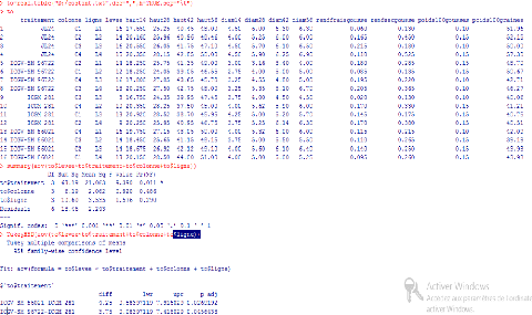
summary(aov(to$111.aut14---to$traitement+to$colonne+to$ligne)j
Df Sum Sq Mean Sq F value Pr(7F) to$traitemernt 3 2.616 .8719
0.340 0.797
to$colonne 3 0.650 0.2166 0.085 0.966
to$ligne 3 6.018 2.0060 0.783 0.545
Residuals 6 15.367 2.5612
7 Tu]ceyHSD(eov(to$Yaaut14--to$traitement+to$colonue+to$ligrne)
)
Tnkey multiple comparisons of means 95% family-wise confidence
level
Fit: aov(formula = to$haut14 -- to$traitement + to$colonne +
to$ligne}
$'to$traiteraent'
di ff lwr upr p ad]
ICGV-SM 86021-ICGM 281 -0.31125 -4.22866 3.60616 0.9919805
TCGV-SM 96722-ICGM 281 -0.93000 -4.84741 2.98741 0.8425268
JT.24-ICGM 281 0.11000 -3.80741 4.02741 0.9996327
ICGV-SM 96722-ICGV-SM 85021 -0.61875 -4.53516 3.29855
0.9440941
JL24-ICGV-SM 86021 0.42125 -3.49616 4.33866 0.9807909
J1.24-ICGV-SM 96722 1.04000 -2.87741 4.95741 0.7964442
S `to$colorine `
di ff lwr upr p ad]
-C1 0.09125 -3.82616 4.00855 0.9987900
C3-C1 -0.24250 -4.15991 3.67491 0.9961443 C4-C1 0.32000 -3.59741 4.23741
0.9913056 C3- -0.33375 -4.25116 3.58355 0.9901740 C4- 0.22875 -3.68866 4.14616
0.9967546 C4-C3 0.56250 -3.35491 4.47991 0.9568408
$ to$ligne`
6374434
di ff lwr upr p adj
1.2-1.1 0.753125 -3.478162 4.984412
0.9232532 1.3-1.1 0.390000 -3.555884 4.435884 0.9859568 1-4-1-1 1.700525
-2.530662 5.931912 0.5468995 1.3-1.2 -0.353125 -4.079507 3.353257 0.9853985
1.4-1-2 0.947500 -2.969910 4.864910 0.8354758 1.4-1.3 1.310625 -2.405757
5.027007 0.
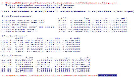
summary(aov(to$191aut28--to$traitement+to$colonne+to$1igne)}
Df Sum Sq Mean Sq F value Pr(7Y) to$traitement 3 1.572 0.524
0.237 0.867
to$colonne 3 9.106 3.035 1.374 0.338
ta$ligne 3 7.406 2.469 1.117 0.413
Residuals 6 13.258 2.210
7 Tu]ceyHS0(aov(to$liaut28-to$traitement+to$colonne+to$ligne)j
Tuke y multiple comparisons of means 95% family-wise confidence
level
Fit: aov(formula = to$haut28 -- to$traitement + to$colonne +
to$ligne) S'to$traitement'
di ff lwr upr p adj
ICGV-SM 86021-ICGM 281 0.2875 -3.351109 3.926109 0.9921091
ICGV-SM 96722-1CGM 281 -0.4800 -4.118509 3.158609 0.9558429
J1.24-ICGM 281 -0.4150 -4.053509 3.223609 0.9772932
ICGV-SM 96722-ICGV-SM 86021 -0.7675 -4.406109 2.871109
0.8817034
J1.24-ICGV-SM 86021 -0.7025 -4.341109 2.935109 0.9053114
JL24-ICGV-SM 96722 0.0650 -3.573509 3.703609 0.9999051
S'to$colonne'
cliff lwr upr p ad]
-C1 -0.4350 -4.073509 3.203509
0.9740653 C3-C1 -0.6925 -4.331109 2.946109 0.9087212 C4-C1 1.2700 -2.358509
4.908509 0.6442196 C3- -0.2575 -3.896109 3.381109 0.9942840 C4- 1.7050
-1.933609 5.343609 0.4338747 C4-C3 1.9525 -1.676109 5.601109 0.3318308
$'to$ligne'
cliff 1wr up= p adj
L2-L1 0.1195833 -3.810563 4.049730
0.9995331 L3-L1 0.9953333 -2.752605 4.753272 0.7975033 1.4-1.1 1.6670833
-2.253063 5.597230 0.5076144 L3-L2 0.8757500 -2.575137 4.327637 0.8152554
1.4-1.2 1.5475000 -2.091109 5.186109 0.5056721 1.4-1.3 0.6717500 -2.780137
4.123637 0. 9433799
41
7
summary(aov(to$19..aut42--to$traitement+to$colonne+to$ligue)}
|
Df Sum Sq
|
Mean Sq F value
|
Pr(7E)
|
|
|
|
|
|
|
|
to$traitement
|
3 23.740
|
7.913 10.113
|
0.00922
|
w w
|
|
|
|
|
|
|
to$colonne
|
3 3.133
|
1.044 1.335
|
0.34818
|
|
|
|
|
|
|
|
to$ligne
|
3 18.737
|
6.246 7.982
|
0.01622
|
|
|
|
|
|
|
|
Residuals
|
6 4.695
|
0.782
|
|
|
|
|
|
|
|
|
Signif. codes:
|
0
|
0.001 'k,' 0.01
|
`w: 0.05
|
L.P.
|
|
0.1
|
`
|
'
|
1
|
7 TukeyHSD(aav(ta$naut42--to$traitement+ta$colonne+ta$ligne)}
Tukey multiple comparisons of means 95% family-wise confidence
level
Fit: aov(fat-ncila = to$baut42 -- to$traitement +
to$colonne + to$ligne}
$ ' t o $ t rai t ement '
cliff lwr upr p adj
|
ICGV-SM 86021-ICGM 281
|
|
3.3050
|
1.13970527
|
5.470295
|
0.0074346
|
|
ICGV-SM 96722-ICGM 281
|
|
2.4250
|
0.25970527
|
4.590295
|
0.0312651
|
|
JL.24-ICGM 281
|
|
2.2275
|
0.06220527
|
4.392795
|
0.0446031
|
|
ICGV-SM 96722-ICGV-SM
|
86021
|
-0.8800
|
-3.04529473
|
1.285295
|
0.5388629
|
|
JL24-ICGV-SM 06021
|
|
-1.0775
|
-3.24279473
|
1.087795
|
0.3895739
|
|
JL24-ICGV-SM 96722
|
|
-0.1975
|
-2.36279473
|
1.967795
|
0.9880262
|
|
$ to$calann.e'
di ff
|
lwr
|
upr
|
p adj
|
|
-C1
|
0.7950
|
-1.3702947
|
2.960295
|
0.6104511
|
|
C3-C1
|
0.8500
|
-1.3152947
|
3.015295
|
0.5637882
|
|
C4-C1
|
1.2125
|
-0.9527947
|
3.377795
|
0.3059285
|
|
C3-
|
0.0550
|
-2.1102947
|
2.220295
|
0.9997279
|
|
C4-
|
0.4175
|
-1.7477947
|
2.582795
|
0.9056290
|
|
C4-C3
|
0.3625
|
-1.8027947
|
2.527795
|
0.9346887
|
|
$ to$ligne'
cliff
|
lwr
|
upr
|
p adj
|
|
1.2-1.1
|
-1.33375
|
-3.€725356
|
2.005036
|
0.2936252
|
|
1.3-1.1
|
0.60600
|
-1.6303068
|
2.842307
|
0.7869761
|
|
1.4-1-1
|
1.63875
|
-0.700035€
|
3.977536
|
0.1719055
|
|
L3-L2
|
1.93975
|
-0.1144289
|
3.993929
|
0. 0625766
|
{
7
summary(aov(to$11..aut56--to$traitement+to$colonne+to$ligrie)}
|
Df Sum Sq
|
Mean Sq F
|
value
|
Pr (7F).
|
|
|
|
|
|
ta$traitement
|
3 23.795
|
7.932
|
5.947
|
0.0314
|
|
|
|
|
|
ta$colonne
|
3 1.136
|
0.379
|
0.284
|
0.8355
|
|
|
|
|
|
to$ligne
|
3 9.580
|
3.193
|
2.394
|
0.1670
|
|
|
|
|
|
Residuals
|
6 8.002
|
1.334
|
|
|
|
|
|
|
|
Signif. codes:
|
0 swww:
|
0.001 'ww'
|
0.01
|
`w' 0.05
|
0.1
|
'
|
·
|
1
|
7 TukeyISD(aov(to$11aut56---to$traitement+to$colonrie+to$ligne)
Tukey nuiltiple comparisons of means 95% family-wise confidence level
|
Fit: aov ( forriui1a = to$baut56 -- to$traitement
di ff
$ ` t o $ t rai t ement `
|
+ ta$colonne
|
+ to$ligne)
|
|
ICGV-SM 86021-ICGM 281
|
3.2750
|
mw=-
wr3.2750 0.4481427
|
upr
6.1018573
|
p adj
0.0269967
|
|
ICGV-SM 96722-ICGM 281
|
1.0250
|
-1.8018573
|
3.8518573
|
0.6189278
|
|
TL24-ICGM 281
|
2.1025
|
-0.7243573
|
4.9293573
|
0.1435777
|
|
ICGV-SM 96722-ICGV-SM 86021
|
-2.2500
|
-5.0768573
|
0.5768573
|
0.1154299
|
|
TL24-ICGV-SM 86021
|
-1.1725
|
-3.9993573
|
1.6543573
|
0.5240506
|
|
.31.24-ICGV-SM 96722
|
1.0775
|
-1.7493573
|
3.9043573
|
0.5845832
|
|
$`to$colonne`
di ff
|
lwr
|
upr
|
p adj
|
|
-C1
|
0.4525
|
-2.374357
|
3.279357
|
0.9420534
|
|
C3-C1
|
-0.2000
|
-3.026857
|
2.626857
|
0.9942885
|
|
C4-C1
|
-0.2000
|
-3.026857
|
2.626857
|
0.9942885
|
|
C3-
|
-0.6525
|
-3.479357
|
2.174357
|
0.8526935
|
|
C4-
|
-0.6525
|
-3.479357
|
2.174357
|
0.8526935
|
|
C4-C3
|
0.0000
|
-2.826857
|
2.826857
|
1.0000000
|
$`to$ligne`
|
di ff
|
lwr
|
upr
|
p adj
|
|
L2-L1
|
-1.3554167
|
-4.4087715
|
1.697938
|
0.4740169
|
|
L3-L1
|
-0.9726667
|
-3.8922323
|
1.946899
|
0.6739070
|
|
L4-L1
|
0.5420833
|
-2.5112715
|
3.595438
|
0.9237623
|
|
L3-L2
|
0.3827500
|
-2.2990423
|
3.064542
|
0.952
|
42
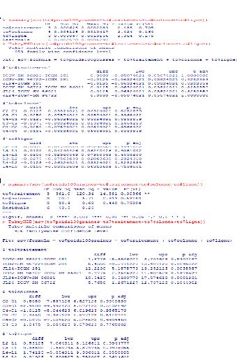
summary(aov(to$diam14--to$traitemeut+to$colonne+to$lzgrae) Df Sum
Sq Mean Sq F value Pr(7E)
to$traztement 3 3.637 1.2222 34.912 0.000341 WWW
to$colonne 3 0.137 0.0456 1.313 0.354231
to$1zgne 3 0.233 0.0777 2.238 0.184413
Residuals 6 0.208 0.0347
Siquif. codes: ',r
x,r. 0.001 0.01 -f.. 0.05 0.1 1
7 TulceyHSD(sov(to$diaml4--to$traitemeot+to$colonue+to$lique)j
rake y multiple conpart s ans of means 95% family-wise confidence 1 eve 1
Fit: aov (fo rmnl a = t o $ di aml 4 -- t o $ t raz t emeut +
to$colonne + t o $ 1 z gne )
$'to$traitement'
di ff 1wr upr p adj
ICGV-SM 86021-ICGM 281 0.0000 -0.45612052 0.4561205 1.0000000
ICGV-SM 96722-ICGM 281 -0.8750 -1.33112052 -0.4188795
0.0023016
1.24-ICGM 281 0.4375 -0.01862052 0.8936205 0.0589150
ICGV-SM 96722-ICGV-SM 86021 -0.8750 -1.33112052 -0.4188795
0.0023016
.71-24-ICGV-SM 86025 0.4375 -0.01862052 0.8936205 0.0589150
.71-1.24-ICGV-SM 96722 1.3125 0.85637948 1.7686205
0.0002477
S`to$colonne'
cliff 1wr upr p adj
-C1 -0.1875 -0.6436205 0.2686205
0.5305761 C3-C1 -0.0625 -0.5186205 0.3936205 0.9620537 C4-C1 0.0625 -0.3936205
0.5186205 0.9620537 C3- 0.1250 -0.3311205 0.5811205 0.7816426 C4- 0.2500
-0.2061205 0.7061205 0.3206306 C4-C3 0.1250 -0.3311205 0.5811205 0.7816426
S`to$lzgne`
di ff 1wr upr p adj
1.2-1.1 -0.23958333 -0.7322498 0.2530831 0.4064571 1-3-1.1
0.06666667 -0.4044126 0.5377459 0.9585268 1-4-1-1 0.01041667 -0.4822498
0.5030831 0.9998428 1.3-1.2 0.30625000 -0.1264639 0.7389639 0.1669139
7 summary (ao T(to$dlr~m78-to$traite]Rent+to$color me+to$] igme )
Df Sum Sq Mean Sq F value Pr(7F)
t otraitement 3 4.377 1.4589 2.554 0.143
to$colonne 3 0.590 0.1966 0.358 0.786
t o$ligne 3 0.687 0.2289 0.416 0.748
Residuals 6 3.299 0.5498
TukeyISD(aov(ta$dlam28-to$traitement+to$calonne+to$llgne)j
Tukey multiple comparisons of means 95% family-wise
confidence level
Fit: aov(formonila = to$diam28 ^- to$traiterit + tocolonue +
to$ligne}
$-to$traitement`
duff lwr upr p adj
ICGV-SM 86021-ICGM 281 0.2625 -1.5524342 2.0774342 0.9559766
ICGV-SM 96722-ICGM 281 -0.7025 -2.5174342 1.1124342 0.5737798
SL24-ICGM 281 0.7450 -1.0699342 2.5599342 0.5316254
ICGM-SM 96722-ICGV-SM 86021 -0.9650 -2.7799342 0.8499342
0.3418899
J7.24-ICGV-SM 86021 0.4825 -1.3324342 2.2974342 0.7958142
JI.24-ICGV-SM 96722 1.4475 -0.3674342 3.2624342 0.1146552
$'-to$colonne'
cliff lwr upr p adj
-C1 -0.1850 -1.999934 1.629934
0.9835134 C3-C1 0.0125 -1.802434 1.827434 0.9999946 C4-C1 0.3475 -1.467434
2.162434 0.9073055 C3- 0.1975 -1.617434 2.012434 0.9801291 C4- 0.5325 -1.282434
2.347434 0.7472488 C4-C3 0.3350 -1.479934 2.149934 0.9156441
$'to$lign
duff lwr upr p adj
L2-L1 0.1766667 -1.78368E 2.137020
0.9884361 L3-1.1 0.2006667 -1.673789 2.075123 0.9810341 L4-L1 0.5841667
-1.376186 2.544520 0.7389248 L3-L2 0.0240000 -1.697798 1.745798 0.9999549 L4-L2
0.4075000 -1.407434 2.222434 0.8621654 L4-L3 0.3835000 -1.338298 2.105298
0.8648165
43
7 summarr(aov(to$diam42-to$traitement+to$colonne+to$ligrie)j
t o $ t rai t eurent t o$ col ohne t o$ 1 i gne Residuals
Of
|
Sum Sq
|
Mean Sq F
|
value
|
Pr (7F)
|
|
3
|
5.254
|
1.7512
|
3.068
|
0.113
|
|
3
|
0.449
|
0.1497
|
0.262
|
0.850
|
|
3
|
0_483
|
0.1510
|
O_282
|
0.837
|
|
6
|
3.425
|
0.5709
|
|
|
7 TulceyHSD(aov(to$diam42-to$traitement+to$colonne+to$ligme))
Tulcey rain t iple comparisons of means 95%
faxai 1 y-wise confidence 1 eve 1
Fit: aov(forxmula to$diara42 -- to$traitement + to$colonne +
to$ligne}
$ - t o $ t rai t ement
I CGV- SM 8 6 0 2 1 -ICGM 281 I CGV- SM 9 6 7 2 2 -ICGM 281
al.24-ICGM 281
I CGV- SM 0 6 7 2 2- ICGV- SM 01T.24-ICGV-SM 86021
01T.24-ICGV-SM 96722
|
cliff
|
1wr
|
upr
|
p adj
|
|
0.2150
|
-1.6344422
|
2.0644422
|
0.9760343
|
|
-0.8600
|
-2.7094422
|
0.9894422
|
0.4395623
|
|
0.7275
|
-1.1219422
|
2.576-9422
|
0.5623271
|
|
8.6021
|
-1.0750
|
-2.9244422
|
0.7744422
|
0.2809791
|
|
0.5125
|
-1.3369422
|
2.3619422
|
0.7762867
|
|
1.5875
|
-0.2619422
|
3.4359422
|
0.0890269
|
lwr
- 1.814442
- 1.924442
- 1.48.5942
- 1.959442
- 1.521942
- 1.411942
.-C1
.C3-C1
.C4-C1
C3 -
C4-
C4 -C3
$`to$colonne'
cliff
0.0350
- 0.0750 0.3625
- 0.1100 0.3275 0.4375
|
upr
|
p adj
|
|
1.884442
|
0.9998872
|
|
1.774442
|
0.9989001
|
|
2.211942
|
0.9015007
|
|
1.739442
|
0.9965734
|
|
2.176942
|
0.9242741
|
|
2.286942
|
0.8438455
|
$ `to$ligrne `
|
L2-1.1 L3 -L1 L4-1-1 L3-L2 L4-L2 L4-L3
|
cliff 0.4254167 0.2005667 0.4479167
- O.2247500 0.0225000 0.2472500
|
lwr
- 1_572209
- 1.709429
- 1.549709
- 1.979285
- 1.825942
- 1.507285
|
upr g adj
2.423043 0_8788701 2.110762 0.9820266 2.445543 0.8525126 1.529785
0.9685273 1.871942 0.9999700 2.001785 0.9590069
|
} Summary(ao(to$dlam56-to$traitement+to$colonne+to$11gue) Df Sum
Sq Mean Sq F value Pr (7F)
t o$traitement 3 3.213 1.0710 1.334 0.348
t o$colonne 3 0.375 0.1252 0.156 0.922
t o$ligne 3 1.662 0.5540 0.690 0.591
Residuals 6 4.817 0.8028
7 TukeyHSD(aov(to $diam56-to$traitement+to$colonne+to$ligne) }
Tukey multiple comparisons of means 95% family-wi se confidence
level
Fit: aov(formula = to$diam56 -- to$traitement + to$colonne +
to$ligne} $'to$traitemient'
dlff
ICGV-SM 86021-ICGM 281 0.1625
ICGV-SM 96722-ICGM 281 -0.4500
Jî.24-ICGM 281 0.8000
ICGV-SM 96722-ICGV-SM 86021 -0.6125
J1.24-ICGV-SM 86021 0.6375
J1..24-ICGV-SM 96722 1.2500
lwr
- 2.0307414
- 2.6432414
- 1.3932414
- 2.8057414
- 1.5557414
- 0.9432414
upr p adj
|
2.355741
|
0.9934614
|
|
1.743241
|
0.8895773
|
|
2.993241
|
0.6149053
|
|
1.580741
|
0.7724921
|
|
2.830741
|
0.7521779
|
|
3.443241
|
0.2940266
|
$`to$colonne'
cliff lwr upr p adj
-C1 0.1125 -2.080741 2.305741 0.9977887
C3-C1 0.2375 -1.955741 2.430741 0.9804045 C4-C1 0.4125 -1.780741 2.605741
0.9114576 C3- 0.1250 -2.068241 2.318241 0.9969792 C4- 0.3000 -1.893241 2.493241
0.9622380 C4-C3 0.1750 -2.018241 2.368241 0.9918807
$`ta$ligne`
diff lwr upr p adj
L2-L1 0.21875 -2.150222 2.587722
0.9875933 L3-L1 0.23000 -2.035170 2.495170 0.9836955 L4-L1 0.88125 -1.487722
3.250222 0.6014814 L3-L2 0.01125 -2.069442 2.091942 0.9999974 L4-L2 0.66250
-1.530741 2.855741 0.7314969 L4-L3 0.65125 -1.429442 2.731942 0.7113970
44
| 

