
KIGALI INDEPENDENT UNIVERSITY (ULK)
SCHOOL OF ECONOMICS AND BUSINESS STUDIES
DEPARTMENT OF ECONOMICS
POBox: 2288 KIGALI-RWANDA
AFFECTING AGGREGATE CONSUMPTION
EXPENDITURE IN RWANDA
PERIOD: 1995-2015
WELFARE
DETERMINANTS
A research thesis submitted in the partial fulfillment of the
requirements of the award of bachelor's degree in economics
Submitted by: -NIZEYIMANA Alphonse: 31075
SUPERVISOR: Prof. Dr. RUFUS Jeyakumar
Kigali, September, 2016
III
DECLARATION
I, NIZEYIMANA Alphonse hereby declare that this dissertation
entitled «Welfare implication of determinants affecting aggregate
consumption expenditure in Rwanda: 1995-2015» is my own work and
it has not been submitted anywhere for the award of any degree.

NIZEYIMANA Alphonse
Tel: +250788851921/+250787077701
Email:
nzmnalphonse@gmail.com
iv
APPROVAL
This is to certify that this dissertation work entitled
«Welfare implication of determinants affecting aggregate
consumption expenditure in Rwanda 1995-2015» is original research
conducted by Mr. NIZEYIMANA Alphonse under my supervision and
Guidance as a University full lecturer.

Supervisor: Prof. Dr. RUFUS Jeyakumar
Full Professor and Dean of the School of Economics and Business
Studies at Kigali Independent University (ULK)
Email: deanfebskigali@ulk.ac.rw
Tel: +250788303668/+250788620205

To my brothers, sisters,
friends and beloved
relatives
To my parents with my
whole family for their
endless
affection,
DEDICATION
V
AKNOWLEDGMENT
I would like first to acknowledge and thank God for loving and
blessing me since my birth until now.
I thank particularly Prof. Dr. RUFUS Jeyakumar
who devoted part of his time to the supervision of this work. His
invaluable guidance contributed to the successful completion of this
research.
I would like to expand my thanks to my beloved HABIMANA
Canisius's whole family.
I would like to expand my thanks to brothers and best friends:
Mr. NSABIMANA Amiable, Mr. HATEGEKIMANA Jean Baptiste,
Mr. HAREMIMANA Joseph, Mr. NGIRIMANA Benjamin and their
families who more contributed to the achievement of this work.
Thanks go to my beloved family Mme
NYIRAMBARUSHIMANA Alexandrine and my first bone BUSINGYE Thea
Isabelle who all encouraged me during my studies. Thanks go to my
friends, colleagues and classmates precisely in the department of economics for
making my student life enjoyable.
vi
May God bless them!
VII
LIST OF ACCRONYMS AND ABBREVIATIONS
%: Percentage
AD: Aggregate Demand
ADF: Augmented Dickey-Fuller
APC: Average Propensity to Consume
APC: Average Propensity to Consume
AS: Aggregate Supply
BNR: Bank National du Rwanda
Co: Autonomous Consumption
CPI: Consumer Price Index
DHS: Demographic Health Survey
?: Change (increase or decrease)
e: nominal exchange rate
EXCHR: Exchange rate
Frw: Rwandan Francs
GCE: Gross Consumption Expenditures
GDP: Gross Domestic Product
GNP: Gross National Product
i.e.: It means
INF: Inflation rate
INT: interest rate
LDC: Less Developed Country
LM: Lagrange Multiplier
MPC: Marginal Propensity to Consume
NDP: Net Domestic Product
VIII
NNP: Net National Product
OLS: Ordinary Least square
PCE: Personal consumption expenditures
PP: Philip-Peron Calculated value
R2: R-square
SACCOs: Savings and Credit Cooperative
Organizations
U L K: Kigali independent university
WWW: World Wide Web
X-M: Export minus Import
Yd: Disposable income
å: Real exchange rate
ix
ABSTRACT:
The research on welfare implication of determinants affecting
aggregate consumption expenditure was conducted by taking Rwanda as an area of
study, period 1995- 2015. The researcher's main purpose was to evaluate the
impact of gross domestic product, lending interest rate, inflation rate and
exchange rate on consumption expenditure in economy. To achieve the desired
objectives, the researcher analyzed how independent variables of the Gross
consumption expenditure (GDP, Lending Interest rate, Inflation rate and
Exchange Rate) work and how they affect the dependent variable (GCE). Augmented
Dickey-Fuller (ADF) and Phillips- Peron (PP) tests were used for stationarity
test. Engle- Granger two steps procedure and the Johansen Maximum Likelihood
Methodology were used to see whether variables are co-integrated or not. The
series analysis was done using Eviews 8 Software. Those tests revealed that
there is co-integration among variables. The researcher found that the economic
authorities in Rwanda use different tools of monetary policy and fiscal policy
in order to stabilize the economy, using determinants such as: money supply,
government spending, credit control, interest rates and other monetary and
fiscal measures can be manipulated by the economic authorities of Rwanda to
maintain welfare of the society.
Keywords:
Gross consumption expenditure(GCE), Inflation rate
measured by Consumer Price Indices(CPI), Exchange rate, Lending interest rate,
, Gross domestic product(GDP).
X
LIST OF TABLES
Table 1: Status and trends of gross
consumption expenditure, Gross domestic product, Interest rate 29
Table 2: Stationarity at Level 39
Table 3: Stationarity at first difference
40
Table 4: Stationarity at second difference
41
Table 5: Long run Johansen Co-integration
test output 55
Table 6: Long run output effect of changes in
GDP, INT, INF, and EXCHR on Gross 56
Table 7: Short run relationship effect of
changes in GDP, INT, INF, and EXCHR on Gross 57
Table 8: Serial correlation tests 60
Table 9: Heteroscedasticity Test 60
Table 10: Ramsey reset Test 61
xi
LIST OF FIGURES
Figure 1: Inflation Keynesian View 23
Figure 2: Status and trends of gross
consumption expenditure, Gross domestic product, Interest rate 30
Figure 3: Jarque-bera Test output 59
Figure 4: Cusum test 62
XII
TABLE OF CONTENTS
APPROVAL iv
LIST OF TABLES x
LIST OF FIGURES xi
GENERAL INTRODUCTION 1
1.Background of the study 1
2.Significance of the study 2
3.Scope and period of the study 3
4.Problem statement 3
5.Hypothesis 5
6.Objectives of the study 6
6.1General objectives 6
6.2Specific objectives 6
7.Research methodology 6
7.1Techniques 6
7.1.a. Documentary technique 7
7.1.b. Interview technique 7
7.2 Methods 7
7.2.a. Statistical method 7
7.2.b. Analytical method 7
7.2.c Historical method 8
7.2.d Comparative method 8
7.2.e. Econometric method 8
8. Organization of the study 8
CHAP I: REVIEW OF LITERATURE 9
INTRODUCTION 9
Definition of the key concepts 9
1.1 Welfare: 9
1.1.a. The Genesis of the Welfare State 9
1.2 Consumption 10
1.2. a. Autonomous consumption 11
XIII
1.2. b. Marginal propensity to consume 11
1.2. c Disposable income 12
1.3 National income 13
1.3.a. Definitions of National Income: 13
1.3.b Concepts of National Income: 16
1.4 Interest rate 19
1.4. a. Nominal Interest Rate 19
1.4.b Real Interest Rate 20
1.4. c Effective interest rate 20
1.5. Inflation rate 20
1.5.1. Causes of inflation 21
1.5.1.a. The cost push-inflation (On the supply side) 21
1.5.1. b Demand-Pull Inflation (On the demand side) 22
1.5.2 Keynesian inflation theory 23
1.6. Exchange rates 24
1.6. a. Nominal exchange rate (e) 24
1.6.b. Real exchange rate (å) 24
CHAPTER 2 ANALYSIS OF THE STATUS AND TRENDS OF
DETERMINANTS 27
INTRODUCTION 27
2.1. Evolution of gross consumption expenditure in Rwanda
1995-2015 27
CHAPTER 3 ECONOMETRIC ANALYSIS OF THE RELATIONSHIP OF
35
INTRODUCTION 35
3.1 Model specification 35
3.1.1 Hypothesis of the model 36
3.1.2. Expected signs 37
3.1.3 Test and analysis of the data 37
3.2. Data processing 37
3.2.1. Unit root tests 37
3.2.1.a. Why testing stationarity? 37
3.2.1.b. Interpretation of stationarity test 53
3.3 Estimation of long run model 53
xiv
3.3.1 Co-integration test 53
3.3.2 Interpretation of Johansen Co-integration test output
55
3.3.3 Long run output 56
3.4 DIAGNOSTIC TESTS 58
3.4.1 Jarque-bera test (Normality test) 59
3.4.2 Breusch-Godfrey test (Serial correlation LM test)
60
3.4.3 Heteroscedasticity Test (Breusch Pagan Godfrey) 60
3.5 STABILITY TESTS 61
3.5.1 Ramsey reset test 61
3.5.2 Recursive estimates (OLS only): Cusum test 61
CONCLUSION ..64
SUGGESTIONS 64
REFERENCES ..66
APPENDICES 68
APPENDICES I 69
APPENDICES II 71
1
GENERAL INTRODUCTION 1.Background of the
study
In Rwandan economy as other economic systems of different
countries, among several key macroeconomic variables that determine aggregate
output, aggregate consumption appears to be an output determining variable that
has attracted a lot of attentions and studies. As one of the fundamental
components of gross national product (GNP) & gross domestic product (GDP)
and a major variable for measuring economic growth, consumption expenditure and
the nature of the consumption function have engaged much of the macroeconomic
debate dating back to John Stuart Mills and the classical economists of the
18th & 19th centuries, J.M. Keynes, Milton Friedman,
Franco Modigliani, James Duesenberry, Simon Kuznet etc. in the early to
mid-19th century.
This is so because consumption expenditure accounts for about
2/3of aggregate expenditure in virtually all economies. Consumption
according to (Blanchard O. 2003) is the act of using goods and services for the
purpose of satisfying man's innumerable needs. This encompasses the importance
of consumption in welfare. The aggregate consumption expenditure level which
includes expenditure on durable and nondurable goods shows the general position
of an economy. Neoclassical economists generally consider consumption to be the
final purpose of economic activity and thus, the level of consumption per
person is viewed as a central measure of an economic productive success. The
study of consumption behavior plays a central role in both macroeconomics and
microeconomics. Macroeconomists are interested in aggregate consumption for two
reasons. First aggregate consumption determines aggregate saving because
aggregate saving defined as the portion of income not consumed, flows through
the financial system to create the national supply of capital.
It follows that the aggregate consumption and saving behavior
have a powerful influence on economy's long term productive capacity. Second,
since consumption expenditure accounts for most of national output,
understanding the dynamic of aggregate consumption expenditure is essential to
understanding macroeconomic fluctuation and the business cycle. Microeconomists
have studied consumption behavior for many reasons such as using consumption
data to measure poverty, to examine the household's preparedness for retirement
or to test theories of competition in retail industries. A rich variety of
household level data sources in Rwanda allowed the researcher in this work to
examine household spending behavior, which has also been utilized to examine
interactions between
2
consumption and other economic behaviors such as job seeking
or educational attainment in Rwanda. From the foregoing, it is important to
point out that both the government of Rwanda and household sectors of the
economy engage in consumption expenditure. The determinants of consumption
expenditure have been influenced by a number of other economic variables. To
study factors both quantitative and qualitative such as income, wealth,
interest rate, capital gain, liquid assets, etc. that can influence
consumption, as whatever influences consumption expenditure, plays a major role
in the process of economic growth in every economy and that of Rwanda as well.
Consumption decision and behavior is crucial for both short run and long run
analysis because of its role in determining aggregate output.
2.Significance of the study
The general interest of this study is to conduct a research
and the report can help understand the content of welfare implication of
determinants affecting aggregate consumption expenditure in Rwanda. It is very
important to understand household consumption and its determinants because
consumption and saving behavior have a powerful influence on economy's long
term productive capacity. It can help the society of Rwanda to know the effects
and the level of consumption expenditure so that they can manipulate it.
To the researcher
This study helped the researcher to be more acquaint with the
important role of income, interest rate, inflation rate as well as exchange
rate in influencing consumption decision. This can help also to know that as
increase in income encourages consumption as well as savings. As Rwandan who
has observed different problem in our society, a researcher has been interested
to undertake this work.
To Rwanda community
It can help the community to know how to behave in daily life;
therefore it helps to know how the income determines the level of consumption.
It helps educated people to take seat and introspect to which extent the level
of savings can really be in order to enhance the level of economic growth. This
study viewed as source of documentation to the future researchers and to
students taking similar field.
To ULK
This study also served to the Kigali Independent University
economic Students when they will be choosing their topics to prepare their
dissertations in coming days. The realization of this work complies
3
with the academic requirement by which any student completing
the provided undergraduate program of course has to conduct a research, compile
and present a dissertation in order to be awarded a bachelor's degree.
3.Scope and period of the study
This study is addressing on assessment on welfare implication
of determinants affecting aggregate consumption expenditure in Rwanda. We
normally assessed the level of aggregate consumption as a function of income,
interest rate, inflation rate and exchange rate as well such the Rwanda, after
1994 Genocide, the economy was really in recessionary period so that it was not
easy for the community to produce and consume. The research dated from
15st March 2016 and ended on 15th August, 2016 and then
presented on September 06th, 2016.
4.Problem statement
Rwandan economy is struggling for balance of payment deficit
because of high level of imports and lower level of export, the Rwanda currency
which is depreciating day to day, a continuous increase of prices as well as
the high level of lending interest rate. The level of income is normally lower
because of lower level of return of wages and many other factors. This study,
therefore, aims at finding out the trends of key macroeconomic variables that
determine aggregate consumption expenditure in Rwanda from 1995 to 2015. The
theory underpinning this study stems from the nature and relationship between
consumption and income. The most undeniable attention to what has come to be
called the consumption function was first well thought out by John
Maynard Keynes. In less developed counties (LDC) like Rwanda,
consumption expenditures are based on actual income, not full employment or
equilibrium income, important savings and investment determinants include
income, expectations, and other influence beyond the interest rate. These
assumptions imply that the economy can achieve a short-run equilibrium at less
than full-employment production. According to Keynesian theory, changes in
aggregate demand, whether anticipated or unanticipated have their greatest
short run impact on real output and employment, not on price. Rationalizing
rigid prices is hard to do because according to standard microeconomics theory,
real supplies and demands do not change if all nominal prices rise or fall
proportionally. If government spending increases, for example, all other
components of spending remain constant, then output will increase.
Therefore, J.M Keynes's absolute income hypothesis didn't give
account. Milton Friedman emphasized that consumers smooth their expenditure by
borrowing and
4
lending. He posited that consumption is determined by long
term expected income rather than current level of income. He argued that
consumption in one day is determined not by income received on that day but on
the average daily income received for a period. Income consist of a permanent
(anticipated and planned) component and a transitory (windfall gain/unexpected)
component (Anyanwu, 1993). Milton Friedman noted that permanent income or
expected long average income is earned from both human and non-human wealth
consisting of labor income, saved money, debentures, equity shares, and real
estate and consumer durables goods like cars, refrigerators, air conditioner,
TV sets etc. This theory made an important contribution by laying stress on
changes in interest rate and wealth as well as the desire to add to one's
wealth (Forgha, 2008). Many economists have posited that consumption depends on
a person's lifetime income. Franco Modigliani emphasized that income varies
systematically over people's lives and savings allow consumers to move income
from the time in life when income is high to low income lifetime period in
order to smoothen consumption. The life cycle hypothesis is based on household
utility maximizing behavior defined on present and future consumption subject
to a lifetime resources constraint. It assumes that price is constant, interest
rate is stable and consumers do not inherit any asset and as such the wealth
owned by a consumer are his own. It also indicates that consumption in a period
depends on the total resources (wealth) one has to spend over his remaining
lifetime which composes of initial wealth and expected earnings at late stage
in life. (Onuchuku, 1998).
Keynes in his book «The General Theory of
Employment, Interest rate and Money» published in 1936 laid the
foundation of modern consumption theories. Keynes mentioned several subjective
and objective factors which determine the consumption of a society. However, of
all factors, he posited that the level of income determines the consumption of
an individual and the society. He laid stress on the absolute income of an
individual as the major determinant of consumption and as such, his theory was
regarded as the absolute income hypothesis. His theory centered on the
relationship between the Marginal Propensity to Consume (MPC) and
Average Propensity to Consume (APC).
Further, Keynes put forth the fundamental «psychological
law of consumption» according to which he propounded that as income
increases, consumption increases, though not by as much as the increase in
income. In other words, the marginal propensity to consume is less than 1,
means that 0<MPC<1.
Keynes made 3 salient points from his proposition. First,
consumption expenditure depends mainly on absolute income of the current
period. Second, consumption is a positive function of absolute level of current
income and third, the more income derived, the more the consumption expenditure
in that period (Jhingan, 2002).
5
Keynes posited that interest rate does not have an important
role in influencing consumption decision. This stood in stark contrast to the
classical economist who believed that a higher interest rate encourages savings
and discourages consumption (Blare, 1978). Based on conjectures, Keynesian
consumption function is given as C= C0 + bYd, a>0, where C is the
consumption, Yd is disposable income; C0 is consumption when income
is zero (autonomous consumption) and b is the rate of change of consumption due
to change in income called the marginal propensity to consume (MPC). While this
theory has success modeling consumption in the short run, attempt to apply this
model over a long time frame proved less successful. This led to the emergence
of other consumption theories put forth by several economists based on other
key factors which is believed to determine consumption other than income. From
all the reason above the researcher has to conduct this study basing on the
following two questions:
? What is the status and trends of gross consumption
expenditure, income, interest rate, inflation rate and exchange rate from 1995
up to 2015 in Rwanda?
? Is there any relationship between consumption, income,
interest rate, inflation rate and exchange rate from 1995-2015 in Rwanda?
5.Hypothesis
In order to respond to the above mentioned questions in this
statement of the problem, same hypothesis were indicated to guide the
researcher for positive or negative conclusion that can be explained like
anticipation or opinion regarding the result of the study. Another fact is
prediction regarding the possible outcomes from the study in term of the
variable that hypothesis is tentative proposition which is subject verification
through subsequent investigation (CRAWITZ, 2001-198). So the provisionary
answers from the above mentioned questions are the following:
? Trends positions of gross consumption expenditure that is
relative to its associates to which it belongs in Rwanda are upward sloping.
? There is a long run relationship between gross consumption
expenditure and its associates in Rwanda.
6
6.Objectives of the study
This research aims at general and specific objectives and, which
give a sense to the general objective 6.1General objectives
The general objective of this study is to verify the impact of
income, interest rate, inflation rate and exchange rate on gross consumption
expenditure in Rwanda.
6.2Specific objectives
This study pursues the following specifics objectives:
? To identify the relationship between explained and explanatory
variables of the above
mentioned model in Rwanda
? To study and examine the trends of that model.
? To give suggestions to policymakers
7.Research methodology
Research methodology is the general approach which will be
used while conducting the present study. This research methodology refers
systematically to solve the research problem above mentioned. It can be also
defined as analysis of principles of methods rules and postulates employed by a
discipline, and the systematic study of methods that are the main intention of
the research to find out how change can be implemented effectively within an
organization and to suggest some solutions to correct wrong issues (KHOTAR,
2004)
7.1Techniques
In research, techniques are the way used to collect data from
the field. There are many ways of collecting data such as sample size,
questionnaire, documentary, interview and so on. During this work, techniques
that helped the researcher are the following:
7
7.1.a. Documentary technique
This technique is used to collect information from written
sources related to the topic like: Books, Journals, Brochures, Internet,
Reports, archives and so on.
7.1.b. Interview technique
This technique use face to face or telephone by asking
prepared questions to persons from the targeted institutions or groups. These
questions are related to the research that is being undertaken.
7.2 Methods
The method is a set of intellectual operations which enable to
analyze, to understand and to explain the analyzed reality or to structure the
research. To conduct this research, the following methods used:
7.2.a. Statistical method
Statistical method is the application of statistical and
mathematical methods in the field of economics to analyze and describe the
numerical relationship between key economic variables (KHOTAR, 2005). The
results of analysis are tables and figures estimated by a method of ordinary
least squares (OLS), from the parameters of the model that we have
identified.
7.2.b. Analytical method
The analytical method is a generic process combining the power of
the Scientific Method with the use of
formal process to solve any type of problem. It has these nine
steps:
+ Identify the problem to solve.
+ Choose an appropriate process.
+ Use the process to hypothesize analysis or solution
elements.
+ Design an experiment(s) to test the hypothesis.
+ Perform the experiment(s).
+ Accept, reject, or modify the hypothesis.
+ Repeat steps 3, 4, 5, and 6 until the hypothesis is
accepted.
+ Implement the solution.
+ Continuously improve the process as opportunities arise.
8
This method have been used to analyze the data collected,
other information applied to the research and to understanding theoretical
relationship between consumption, income, interest rate, inflation rate and
exchange rate.
7.2.c Historical method
We have used data from recent years and have been able to
interpret them based on historical evidences. Without history and research
materials in the past, this work would not have been able to succeed.
7.2.d Comparative method
In this research, different ways already available to help in
comparing data have been very helpful in analyzing the data in the period under
study.
7.2.e. Econometric method
Econometrics method is the application of mathematics,
statistics and computer science to economic data and is described as the branch
of economic that aims to give empirical content to economic relations.
This method has been used to compute some parameters with E-views
software and have been used in testing the hypotheses in order to determine the
level of significance. Econometrics is the application of mathematical and
statistical methods to economic data and is described as the branch of
economics that aims to give empirical content to economic relations.
8. Organization of the study
This study is composed of the introduction, three chapters and
conclusion. General introduction includes a brief detail of the above mentioned
point from the back ground to the selected methods to be used:
? The first chapter is the literature review
of the key concept, this means all theories related to the topic of
economics.
? The second chapter presents the analysis of
evolution of trends of consumption, income, interest rate, inflation rate and
the exchange rate.
? The third chapter focuses on the
econometric analysis of the impact of income, interest rate, inflation rate and
exchange rate on aggregate consumption expenditure in Rwanda. Finally, there is
conclusion of the work and suggestions to policymakers.
9
CHAP I: REVIEW OF LITERATURE INTRODUCTION
The theoretical framework of this chapter is the theoretical
literatures which explain in deep the different variables of the used model.
The presentation of different researches which was conducted using the same
variables showing the empirical evidences therefore the researcher focused on
the summary of the gaps to fill in the study.
Definition of the key concepts
1.1 Welfare: In this research, a discussion
on welfare occurred to know whether any allocation of resources is efficient or
not. By efficiency in economics a researcher mean whether any state or
situation regarding resource allocation maximizes social welfare. In welfare
economics attempt is made to establish criteria or norms with which to judge or
evaluate alternative economic states and policies from the viewpoint of
efficiency or social welfare. These criteria or norms serve as a basis for
recommending economic policies which will increase social welfare. Thus the
norms established by welfare economics are supposed to guarantee the optimal
allocation of economic resources of the society. Welfare in economics is
defined as a branch of economics that studies how the distribution of income,
resources and goods affects the economic well-being of the community. An
example of welfare economics is the study of how certain health services help
bridge the barrier between different classes of people.
1.1.a. The Genesis of Welfare State
According to Barr 2004, the Welfare State «defies precise
definition». The main reasons are that welfare derives from other sources
besides state activity and there are various modes of delivery of the services
made available to citizens. Some are funded but not produced by the State, some
publicly produced and delivered free of charge, some bought by the private
sector, and some acquired by individuals with the money handed on to them by
the State. Although its boundaries are not well defined, the Welfare State is
used as «shorthand for the state's activities in four broad areas: cash
benefits; health care; education and food, housing, and other welfare
services» (Barr 2004:21). The objectives of the Welfare in economics can
be grouped under four general headings. It should support living standards and
reduce inequality, and in so doing it should avoid costs explosion and deter
behavior conducive to moral hazard and adverse selection. All these objectives
should be achieved minimizing administrative costs and the abuse of power by
those in charge of running it.
10
1.2 Consumption
Consumption is defined as the use of goods and services by
consumer purchasing or in the production of goods. Personal consumption
expenditures (PCE) are measures of price changes in consumer
goods and services. Consumption refers to the expenditures of goods and
services that give satisfaction in the present time. It is the use of resources
to satisfy human needs. Gross consumption expenditure is the use of resources
used to satisfy human needs at current price. Goods that human always use to
satisfy their needs are therefore divided into subcategories.
Durable goods: These are products that are
not quickly consumed and can be conserved along time. These are tangible goods
that tend to last for more than a year. Common examples are cars, furniture,
and appliances. Durable goods constitute about 10-15 percent of consumption
expenditures.
Non-durable goods: These are products that
are consumed immediately which mean they have a short lifespan. These are
tangible goods that tend to last for less than a year. Common examples are
clothing, food, and gasoline. Non-durable goods constitute about 25-30 percent
of consumption expenditures. Services: A type of economic
activity that is intangible not stored and does not result in ownership. A
service is consumed at the point of sale. Services are one of the two key
components of economics, the other being goods. These are intangible activities
that provide direct satisfaction to consumers at the time of purchase. Common
examples include health care, entertainment, and education. Services constitute
about 55-60 percent of consumption expenditures.
This function is used to calculate the amount of total
consumption in the economy. It is made up by autonomous that is not influenced
by current income and induced consumption that is influenced by economy's level
of income. In its most general form, the household's lifetime value function
can be: consumption in `youth' while the second
argument represents consumption in `old age'. Simply,
this function can be written in variety of ways for example, it can be
expressed as C=a+b(Y-T). Again, it can be expressed as C=C0+C1Yd
Where:
C: total consumption
C0: Autonomous consumption
C1: Marginal propensity to consume
Yd: Disposable income (This is the income after
Government taxes and transfer payment)
11
1.2. a. Autonomous consumption
Autonomous consumption also known as exogenous consumption is
defined as expenditures taking place when disposable income levels are at zero.
This consumption is typically used to fund consumer necessities, but causes
consumers to borrow money or withdraw from savings accounts. It is the
consumption expenditure that occurs when income levels are zero. Such
consumption is considered autonomous of income only when expenditure on these
consumables does not vary with changes in income; generally, it may be required
to fund necessities and debt obligations. In the above mentioned function, the
autonomous consumption is shown by C0.
1.2. b. Marginal propensity to consume
In economics, the marginal propensity to consume (MPC) is a
metric that quantifies induced consumption, the concept that the increase in
personal consumer spending (consumption) occurs with an increase in disposable
income (income after taxes and transfers); therefore it is the slope of
consumption function. Because this metric is assumed to be positive, thus a
positive relationship between consumption and income occurs and if income
increases, the level of consumption increases too. However, Keynes mentioned
that the increase of income and consumption is not equal. The Keynesian
consumption function is also known as the absolute income hypothesis as it is
only based on current income and ignores potential future income.
Criticisms of this consumption led to the development of
Milton Friedman's permanent income hypothesis ad Franco Modigliani' lifecycle
hypothesis. The marginal propensity to consume (MPC) cannot be calculated
without disposable income. In the classic Keynesian framework, disposable
income is the income left over after taxes and is divided between consumption
and investment. Suppose that an individual receives an extra 2000 0 Frw and
spends 18000Frw, saving the remaining 2000 Frw. His MPC is 0.9, or
18000/20000.
The effect is said to be marginal because it assumes new
income being introduced to a previously static state. The marginal propensity
to consume was presented in John Maynard Keynes' work "The General Theory of
Employment, Interest, and Money." Keynes titled this work to evoke comparisons
between his general theory of economics and Albert Einstein's theory of general
relativity. Keynes believed his work was as seminal to mathematical economics
as Einstein's was to mathematical physics. MPC was the starting point to
Keynes' central mathematical arguments. Keynes noted that individual
consumption is divided between consumption and investment. He expressed this
argument as Y = C + I. He further
12
stipulated that any marginal increase in income would be
divided between consumption and investment, or OY = OC + OI. Keynes then
extrapolated from this that communities would have a general tendency to spend
a fraction of its new income. He shows this with OC/OY, or marginal consumption
divided by marginal income. The only thing left over from his formula,
investment, would receive the rest. Later on in "The General Theory of
Employment, Interest, and Money," Keynes manipulated the relationship between
income, consumption and investment to justify his multiplier. Later Keynesians
have argued that this multiplier effect is greater for poorer communities,
since they have many goods and services to buy; their marginal propensity to
consume is larger.
1.2. c Disposable income
People can either spend or save their disposable income. When
people are very poor, they cannot afford to save. All of their disposable
income will be spent on buying basic necessities to survive. In fact, some may
have to spend more of their income in order to be able to buy enough food and
clothing and pay for housing.
When people spend more than their income, they are said to be
dissaving. This is because they are either drawing on their past saving or more
likely, borrowing other people's savings. As income rises people are able, to
both spend and save more. As people become richer they buy more and better
quality products. It is interesting to note, however, that whilst the total
amount spent rises with income, the proportion spent tends to fall. For
example: A top class footballer in Rwanda may earn a disposable income of
150,000 Frw a month whilst an unemployed person in Rwanda may live on benefits
of 15,000 Frw a month.
The unemployed person may spend all of the 15000 Frw. The
footballer can clearly afford to spend more and is likely to do so. However,
even if he has a very luxurious lifestyle, it is unlikely that he will spend
all of the 150,000 Frw. If he spends 100,000Frw (a huge amount) he will only be
spending 80% of his disposable income, whilst the unemployed person is spending
100% of his income.
The proportion of income which people spend is sometimes
referred to as the average propensity to consume (APC). It is calculated by
dividing consumption by disposable income. As income rises, expenditure
increases but the APC falls.
13
1.3 National income
National income is an uncertain term which is used
interchangeably with national dividend, national output and national
expenditure. On this basis, national income has been defined in a number of
ways. Commonly, national income means the total value of goods and services
produced annually in a country. In other words, the total amount of income
accruing to a country from economic activities in a year's time is known as
national income.
It includes payments made to all resources in the form of
wages, interest, rent and profits. In this variable, we shall be giving the
detail containing, definitions of national income, concepts of national income,
methods of measuring, national income, difficulties or limitations in measuring
national income, importance of, national income analysis as well as the
inter-relationship among different concept of national Income.
1.3.a. Definitions of National Income:
The definitions of national income can be grouped into two
classes: One, the traditional definitions advanced by Marshall, Pigou and
Fisher; and two, modern definitions. According to Marshall «The agents of
production: Land, labor and capital and organization a country acting on its
natural resources produce annually a certain net aggregate of commodities,
material and immaterial including services of all kinds. This is the true net
annual income or revenue of the country or national dividend.» In this
definition, the word `net' refers to deductions from the gross national income
in respect of depreciation and wearing out of machines. And to this, must be
added income from abroad.
Though the definition advanced by Marshall is simple and
comprehensive, yet it suffers from a number of limitations. First, in the
present day world, so varied and numerous are the goods and services produced
that it is very difficult to have a correct estimation of them. Consequently,
the national income cannot be calculated correctly. Second, there always exists
the fear of the mistake of double counting, and hence the national income
cannot be correctly estimated. Double counting means that a particular
commodity or service like raw material or labor, etc. might get included in the
national income twice or more than twice.
For example, a peasant sells wheat worth .200,000 frw to a
flour mill which sells wheat flour to the wholesaler and the wholesaler sells
it to the retailer who, in turn, sells it to the customers. If each time, this
wheat or its flour is taken into consideration, it will work out to Rs.800, 000
Frw, whereas, in actuality, there is only an increase of .200, 000 Frw in the
national income. Third, it is again not possible
14
to have a correct estimation of national income because many
of the commodities produced are not marketed and the producer either keeps the
production for self-consumption or exchanges it for other commodities.
The Pigouvian Definition:
Arthur Cecil Pigou in the field of Welfare economics
has, in his definition of national income, included that income which
can be measured in terms of money. In the words of Pigou, «National income
is that part of objective income of the community, including of course income
derived from abroad which can be measured in money. This definition is better
than the Marshallian definition. It has proved to be more practical also. While
calculating the national income nowadays, estimates are prepared in accordance
with the two criteria laid down in this definition. First, avoiding double
counting, the goods and services which can be measured in money are included in
national income. Second, income received on account of investment in foreign
countries is included in national income. The Pigouvian definition is precise,
simple and practical but it is not free from criticism. First, in the light of
the definition put forth by Pigou, we have to unnecessarily differentiate
between commodities which can and which cannot be exchanged for money.
Nevertheless, actually there is no difference in the
fundamental forms of such commodities; no matter they can be exchanged for
money. Second, according to this definition when only such commodities as can
be exchanged for money are included in estimation of national income, the
national income cannot be correctly measured. According to Pigou, a woman's
services as a nurse would be included in national income but excluded when she
worked in the home to look after her children because she did not receive any
salary for it. Similarly, Pigou is of the view that if a man marries his lady
secretary, the national income diminishes as he has no longer to pay for her
services.
Thus the Pigovian definition gives rise to a number of
paradoxes. Third, the definition is applicable only to the developed countries
where goods and services are exchanged for money in the market. According to
this definition, in the backward and underdeveloped countries of the world,
where a major portion of the produce is simply bartered, correct estimate of
national income will not be possible, because it will always work out less than
the real level of income. Thus the definition advanced by Pigou has a limited
scope.
15
Fisher's Definition:
Irving Fisher adopted `consumption' as the
criterion of national income whereas Marshall and Pigou regarded it to be
production. According to Fisher, «The National dividend or income consists
solely of services as received by ultimate consumers, whether from their
material or from the human environments. Thus, a piano, or an overcoat made for
me this year is not a part of this year's income, but an addition to the
capital. Only the services rendered to me during this year by these things are
income. Fisher's definition is considered to be better than that of Marshall or
Pigou, because Fisher's definition provides an adequate concept of economic
welfare which is dependent on consumption and consumption represents our
standard of living. But from the practical point of view, this definition is
less useful, because there are certain difficulties in measuring the goods and
services in terms of money. First, it is more difficult to estimate the money
value of net consumption than that of net production. In one country there are
several individuals who consume a particular good and that too at different
places and, therefore, it is very difficult to estimate their total consumption
in terms of money. Second, certain consumption goods are durable and last for
many years.
If we consider the example of piano or overcoat, as given by
Fisher, only the services rendered for use during one year by them will be
included in income. If an overcoat costs 20,000frw and lasts for ten years,
Fisher will take into account only 20,000 frw as national income during one
year, whereas Marshall and Pigou will include 20,000 frw in the national income
for the year, when it is made. Besides, it cannot be said with certainty that
the overcoat will last only for ten years. It may last longer or for a shorter
period. Third, the durable goods generally keep changing hands leading to a
change in their ownership and value too. It, therefore, becomes difficult to
measure in money the service-value of these goods from the point of view of
consumption.
Modern Definitions:
From the modern point of view, Simon Kuznets
has defined national income as «the net output of commodities and services
flowing during the year from the country's productive system in the hands of
the ultimate consumers. On the other hand, in one of the reports of United
Nations, national income has been defined on the basis of the systems of
estimating national income, as net national product, as addition to the shares
of different factors, and as net national expenditure in a country in a year's
time. In practice, while estimating national income, any of these three
definitions may be adopted.
16
1.3.b Concepts of National Income:
There are a number of concepts pertaining to national income
and methods of measurement relating to them. Gross Domestic Product
(GDP): J.M Keynes Defines GDP as the total value of goods and services
produced within the country during a year. This is calculated at market prices
and is known as GDP at market prices. The Governments always plans to spend
during fiscal year therefore, a reduction in planned expenditure decreases the
level of income (GDP). GDP at market price is «the market value of the
output of final goods and services produced in the domestic territory of a
country during an accounting year.» There are three different ways to
measure GDP: Product method, Income method and Expenditure
method, these three methods of calculating GDP yield the same result
because:
National Product = National Income = National
Expenditure.
Product Method: In this method, the value of
all goods and services produced in different industries during the year is
added up. This is also known as the value added method to GDP or GDP at factor
cost by industry of origin.
The Income Method: The people of a country
who produce GDP during a year receive incomes from their work. Thus GDP by
income method is the sum of all factor incomes: Wages and Salaries
(compensation of employees) + Rent + Interest + Profit.
Expenditure Method: This method focuses on
goods and services produced within the country during one year. GDP by
expenditure method includes:
(i) Consumer expenditure on services, durable and non-durable
goods (C)
(ii) Investment in fixed capital such as residential and
non-residential building, machinery, and inventories (I),
(iii) Government expenditure on final goods and services
(G),
(iv) Export of goods and services produced by the people of
country (X),
(v) Less imports (M). That part of consumption, investment
and government expenditure which is spent on imports is subtracted from GDP.
Similarly, any imported component, such as raw materials, which is used in the
manufacture of export goods, is also excluded.
Thus GDP by expenditure method at market prices = C+ I + G + (X -
M), where (X-M) is net export which can be positive or negative.
GDP at Factor Cost: It is the sum of net value added by all producers
within the country. Since the net value added gets distributed as income to the
owners of factors of production, GDP is the sum of domestic factor incomes and
fixed capital consumption (or depreciation). Thus GDP at Factor Cost =
Net value added + Depreciation.
17
GDP at factor cost includes:
(i) Compensation of employees i.e., wages, salaries, etc.
(ii) Operating surplus which is the business profit of both
incorporated and unincorporated firms. [Operating Surplus = Gross Value Added
at Factor Cost--Compensation of Employees--Depreciation]
(iii) Mixed Income of Self- employed. Conceptually, GDP at
factor cost and GDP at market price must be identical. This is because the
factor cost (payments to factors) of producing goods must equal the final value
of goods and services at market prices. However, the market value of goods and
services is different from the earnings of the factors of production. In GDP at
market price are included indirect taxes and are excluded subsidies by the
government. Therefore, in order to arrive at GDP at factor cost, indirect taxes
are subtracted and subsidies are added to GDP at market price. Thus, GDP at
Factor Cost = GDP at Market Price - Indirect Taxes + Subsidies.
Net Domestic Product (NDP):
NDP is the value of net output of the economy during the year.
Some of the country's capital equipment wears out or becomes obsolete each year
during the production process. The value of this capital consumption is some
percentage of gross investment which is deducted from GDP. Thus Net Domestic
Product = GDP at Factor Cost-Depreciation.
Nominal and Real GDP:
When GDP is measured on the basis of current price, it is
called GDP at current prices or nominal GDP. On the other hand, when GDP is
calculated on the basis of fixed prices in some year, it is called GDP at
constant prices or real GDP. Nominal GDP is the value of goods and services
produced in a year and measured in terms of money at current (market) prices.
In comparing one year with another, we are faced with the problem that is not a
stable measure of purchasing power. GDP may rise a great deal in a year, not
because the economy has been growing rapidly but because of rise in prices (or
inflation). On the contrary, GDP may increase as a result of fall in prices in
a year but actually it may be less as compared to the last year. In both 5
cases, GDP does not show the real state of the economy. To rectify the
underestimation and overestimation of GDP, we need a measure that adjusts for
rising and falling prices. This can be done by measuring GDP at constant prices
which is called real GDP. To find out the real GDP, a base year is chosen when
the general price level is normal, i.e., it is neither too high nor too low.
The prices are set to 100 (or 1) in the base year.
Now the general price level of the year for which real GDP is
to be calculated is related to the base year on the basis of the following
formula which is called the deflator index.
18
GDP Deflator:
GDP deflator is an index of price changes of goods and
services included in GDP. It is a price index which is calculated by dividing
the nominal GDP in a given year by the real GDP for the same year and
multiplying it by 100. Gross National Product (GNP): GNP is the total measure
of the flow of goods and services at market value resulting from current
production during a year in a country, including net income from abroad. GNP
includes four types of final goods and services:
(i) Consumers' goods and services to satisfy the immediate wants
of the people;
(ii) Gross private domestic investment in capital goods
consisting of fixed capital formation, residential construction and inventories
of finished and unfinished goods;
(iii) Goods and services produced by the government; and
(iv) Net export of goods and services, i.e., the difference
between value of exports and imports of goods and services, known as net income
from abroad. In this concept of GNP, there are certain factors that have to be
taken into consideration: First, GNP is the measure of money, in which all
kinds of goods and services produced in a country during one year are measured
in terms of money at current prices and then added together. But in this
manner, due to an increase or decrease in the prices, the GNP shows a rise or
decline, which may not be real. The net National Product All this process is
termed depreciation or capital consumption allowance. In order to arrive at
NNP, we deduct depreciation from GNP. The word `net' refers to the exclusion of
that part of total output which represents depreciation. So NNP =
GNP-Depreciation.
NNP at Market Prices:
Net National Product at market prices is the net value of
final goods and services evaluated at market prices in the course of one year
in a country. If we deduct depreciation from GNP at market prices, we get NNP
at market prices. So NNP at Market Prices = GNP at Market
Prices-Depreciation.
NNP at Factor Cost:
Net National Product at factor cost is the net output
evaluated at factor prices. It includes income earned by factors of production
through participation in the production process such as wages and salaries,
rents, profits, etc. It is also called National Income. This measure differs
from NNP at market prices in that indirect taxes are deducted and subsidies are
added to NNP at market prices in order to arrive at NNP at factor cost. Thus
NNP at Factor Cost = NNP at Market Prices-Indirect taxes+ Subsidies
= GNP at Market Prices - Depreciation-Indirect taxes +
Subsidies.= National Income.
19
Normally, NNP at market prices is higher than NNP at factor
cost because indirect taxes exceed government subsidies. However, NNP at market
prices can be less than NNP at factor cost when government subsidies exceed
indirect taxes. Normally, there are a wide number of theories of National
Income and many economists are interested in discussing about such variable.
This study combines of number of theories and these will help the researcher to
maximize analysis on National income n Rwanda.
1.4 Interest rate
Interest rate is the amount charged, expressed as a percentage
of principal, by a lender to a borrower for the use of assets. Interest rates
are typically noted on an annual basis, known as the annual percentage rate
(APR). It was found the lending interest rate is determined by the funding
cost, the loan size, and the efficiency level of microfinances.
Lending rate is the bank rate that usually meets the short- and
medium-term financing needs of the private sector. This rate is normally
differentiated according to creditworthiness of borrowers and objectives of
financing. Interest is money paid by a borrower to a lender for a credit or a
similar liability. It is the charge for the privilege of borrowing money.
Important examples are bond yields, interest paid for bank loans, and returns
on savings. A modern economy is intrinsically linked to interest rates, thus
their importance on the financial markets. Interest rates affect consumer
spending. The higher the rate, the higher their loans will cost them, and the
less they will be able to buy on credit. Interest rates are classified many we
can state: Nominal interest rate, real interest rate, effective interest rate,
and so on.
1.4. a. Nominal Interest Rate
The nominal interest rate is conceptually the simplest type of
interest rate. It is quite simply the stated interest rate of a given bond or
loan. This type of interest rate is referred to as the coupon rate for fixed
income investments, as it is the interest rate guaranteed by the issuer that
was traditionally stamped on the coupons that were redeemed by the
bondholders.
The nominal interest rate is in essence the actual monetary
price that borrowers pay to lenders to use their money. If the nominal rate on
a loan is 5%, then borrowers can expect to pay 5000 frw of interest for every
100,000 frw loaned to them.
20
1.4.b Real Interest Rate
The real interest rate is slightly more complex than the
nominal rate but still fairly simple. The nominal interest rate doesn't tell
the whole story because inflation reduces the lender's or investor's purchasing
power so that they cannot buy the same amount of goods or services at payoff or
maturity with a given amount of money as they can now.
The real interest rate is so named because it states the
«real» rate that the lender or investor receives after inflation is
factored in; that is, the interest rate that exceeds the inflation rate. If a
bond that compounds annually has a 6% nominal yield and the inflation rate is
4%, then the real rate of interest is only 2%. So Nominal interest
rate - Inflation = Real interest rate.
1.4. c Effective interest rate
One other type of interest rate that investors and borrowers
should know is called the effective rate, which takes the power of compounding
into account.
1.5. Inflation rate
Inflation is the rate at which the general level of prices for
goods and services is rising, and, subsequently, purchasing power is falling.
Central banks attempt to stop severe inflation, along with severe deflation, in
an attempt to keep the excessive growth of prices to a minimum. Inflation is a
state of economy in which the general prices of commodities and services become
high. Another way we can say that «too much money chasing too few
goods». The so called consumer price indices are prominently used to
calculate inflation. An increase in the money supply may be called monetary
inflation, to distinguish it from rising prices, which may also for clarity be
called "price inflation". Economists generally agree that in the long run,
inflation is caused by increases in the money supply. Inflationary problems
arise when we experience unexpected inflation which is not adequately matched
by a rise in people's incomes. If incomes do not increase along with the prices
of goods, everyone's purchasing power has been effectively reduced, which can
in turn lead to a slowing or stagnant economy. So someone can ask himself what
exactly causes inflation in an economy. There is not a single, agreed-upon
answer, but there are a variety of theories, all of which play some role in
inflation:
21
1.5.1. Causes of inflation
1.5.1.a. The cost push-inflation (On the supply
side)
Inflation is primarily caused by an increase in the money
supply that outpaces economic growth. Ever since industrialized nations moved
away from the gold standard during the past century, the value of money is
determined by the amount of currency that is in circulation and the public's
perception of the value of that money. When the Central Bank decides to put
more money into circulation at a rate higher than the economy's growth rate,
the value of money can fall because of the changing public perception of the
value of the underlying currency. As a result, this devaluation will force
prices to rise due to the fact that each unit of currency is now worth less.
The same logic works for currency; the less currency there is in the money
supply, the more valuable that currency will be. When a government decides to
print new currency, they essentially water down the value of the money already
in circulation. A more macroeconomic way of looking at the negative effects of
an increased money supply is that there will be more Rwandan currency chasing
the same amount of goods in economy which will inevitably lead to increased
demand and therefore higher prices.
Cost-Push Effect
Another factor in driving up prices of consumer goods and
services is explained by an economic theory known as the `cost-push
effect'. Essentially, this theory states that when companies are
faced with increased input costs like raw goods and materials or wages, they
will preserve their profitability by passing this increased cost of production
onto the consumer in the form of higher prices. Inflation can be categorized
into many but the most current ones are: Demand Pull Inflation this is a kind
of inflation that occurs on demand side where the demand for goods and services
exceed the supply.
Cost Push Inflation: this is a kind of inflation that occurs
on the supply side where price increases due to an increase in price of other
products.
22
Calculation of Inflation
For example, CPI on Jan 1, 2013 is 125 and that on Jan 1, 2014
is 133.75 then inflation for the year 2014 would be:
Or:
Therefore:
The National Debt
In economics, the reason for this is that if there is a
country's debt increases, the government has two options: it can either raise
taxes or print more money to pay off the debt. A rise in taxes will cause
businesses to react by raising their prices to offset the increased corporate
tax rate. Alternatively, should the government choose the latter option,
printing more money will lead directly to an increase in the money supply,
which will in turn lead to the devaluation of the currency and increased
prices.
1.5.1. b Demand-Pull Inflation (On the demand side)
The demand-pull effect states that as wages increase within an
economic system (often the case in a growing economy with low unemployment),
people will have more money to spend on consumer goods. This increase in
liquidity and demand for consumer goods results in an increase in demand for
products. As a result of the increased demand, companies will raise prices to
the level the consumer will bear in order to balance supply and demand. An
example would be a huge increase in consumer demand for a product or service
that the public determines to be cheap. For instance, when hourly wages
increase, many people may determine to undertake home improvement projects.
This increased demand for home improvement goods and services will result in
price increases by house-painters, electricians, and other general contractors
in order to offset the increased demand. This will in turn drive up prices
across the board.
23
1.5.2 Keynesian inflation theory
The eminent economist John Maynard Keynes
theorized a lot about inflation. He postulated that the money supply
had an influence on inflation in a much more complex way than the strict
monetarists suggested. Instead Keynes proposed that inflation was caused in
number of different ways: By demand outstripping supply and pulling inflation
higher, by inflation being built into the system, by higher costs pushing
inflation higher. Below are examples of each of these types of causes of
inflation.

Source: Kahn R (1976) `Inflation-Keynesian View' Scottish
Journal of political Economy: London, UK Figure 1: Inflation Keynesian
View
It was also Keynes's view that inflation expectations were
important. They impact the wage settlements that workers seek and affect other
inflation agreements that are created. These can have a marked effect on future
inflation rates. Furthermore Keynes and his followers have argued that
governments face a trade-off between unemployment and inflation i.e. if you
want full employment you may need to tolerate higher inflation. Indeed, as
Keynes was writing during the Great Depression
(1929-1933), he not surprisingly gave great importance to
reducing unemployment. This thinking paved the way for post-war governments
that were less concerned about creating inflation than their predecessors, as
they saw it as a necessary trade-off to create full employment. It is
interesting that the Keynesian theory of inflation has gone out of fashion.
This is probably related to the rejection of Keynesian thinking in
general which started in the 1970s. However Keynesian ideas
have had something of a renaissance following the Great Recession of 2008 as
governments seek alternative solutions to the problems we now face.
1.6. Exchange rates
The exchange rate between two countries is the price which
residents of those countries trade with each other. Economists distinguish
between two exchange rates: Nominal exchange rate and Real exchange rate.
1.6. a. Nominal exchange rate (e)
This is the relative price of the currency of two countries.
In other words, the nominal exchange rate is the rate at which one currency
trades against another on the foreign exchange market. The nominal exchange
rate e is defined again as the number of units of the domestic currency that
can purchase a unit of a given foreign currency. A decrease in this variable is
termed nominal appreciation of the currency. (Under the fixed exchange rate
regime, a downward adjustment of the rate e is termed revaluation.) An increase
in this variable is termed nominal depreciation of the currency. (Under the
fixed exchange rate regime, an upward adjustment of the nominal rate e
is called devaluation). When people refer to the exchange rate between
two countries, they usually mean the nominal exchange rate. So the nominal
exchange rate can be expressed as:
1.6.b. Real exchange rate (å)
This is the relative price of the goods of two countries. It
tells us the rate at which we can trade the goods of one country for good of
another. The real exchange rate R is defined as the ratio of the price level
abroad and the domestic price level, where the foreign price level is converted
into domestic currency units via the current nominal exchange rate.

24
Where
25
å= Real exchange rate
P* = Price of foreign good
P= Price of domestic good
e= Nominal exchange rate
A decrease in å is termed appreciation of the real
exchange rate, an increase is termed depreciation. The real rate tells how many
times more or less goods and services can be purchased abroad (after conversion
into a foreign currency) than in the domestic market for a given amount. In
practice, changes of the real exchange rate rather than its absolute level are
important. In contrast to the nominal exchange rate, the real exchange rate is
always »floating», since even in the regime of a fixed nominal
exchange rate e, the real exchange rate å
can move via price level changes. Normally, it is the nominal exchange
rate adjusted for inflation. Unlike most other real variables, this adjustment
requires accounting for price levels in two currencies. Standard models of
international risk sharing with complete asset markets predict a positive
association between relative consumption growth and real exchange-rate
depreciation across countries. The striking lack of evidence for this link the
consumption/real-exchange-rate anomaly or `Backus-Smith
puzzle' has prompted research on risk-sharing indicators with
incomplete asset markets. That research generally implies that the association
holds in forecasts, rather than realizations. Independent evidence on the weak
link between forecasts for consumption and real interest rates suggests that
the presence of 'hand-to-mouth' consumers may help to resolve the anomaly.
Developed by James Duesenberry(1946), the relative income hypothesis states
that an individual's attitude to consumption and saving is dictated more by his
income in relation to others than by abstract standard of living; the
percentage of income consumed by an individual depends on his percentile
position within the income.
It is reasonable to say that Adam Smith (1776) has played an
important role in the development of welfare theory. The reasons are at least
two: In the first place, he created the invisible hand idea that is one of the
most fundamental equilibrating relations in economic theory, the equalization
of rates of returns as enforces by a tendency of factors to move from low to
high returns through the allocations of capital to individual industries by
self-interested investors. The self-interest will results in an optimal
allocation of capital for society. He writes: «every individual is
continually exerting himself to find out the most advantageous employment for
whatever capita he can command. It is his advantage, indeed, and not that of
society, which he has in view. But the study of his own advantage naturally, or
rather necessarily leads him to prefer that employment which is most
advantageous to society». Adam Smith does not stop there but notes that
what is true for investment is true in economic activity in general.
26
«Every individual necessarily labors to render the annual
revenues of the society as great as he can. He generally, indeed, neither
intends to promote the public interest, nor knows how much is promoting
it» He concludes: «It is not from the benevolence of the butcher, the
brewer or the baker, that we expect our dinner, but from the regards of their
own interest». The most famous line is probably the following: The
individual is led by an invisible hand to promote an end which was no part of
his own intention. The invisible hand is competition and this ides was present
already in the work of the brilliant and undervalued Irish economist
Richard Cantillon. He sees the invisible hand as embodied in
the central planner, guiding the economy to social optimum.
The second reason why Adam Smith played an important role in
the development of welfare theory is that, an attempt to explain the
«Water and Diamond Paradox», he came across an
important distinction in value theory. At the end of the fourth chapter of the
first book in Adam Smith's celebrated volume The Wealth of Nations
(1776), he brings up a valuation problem that is usually referred
to as the Value Paradox2. He writes.
27
CHAPTER 2: ANALYSIS OF THE STATUS AND TRENDS OF
DETERMINANTS
AFFECTING AGGREGATE CONSUMPTION EXPENDITUTE IN
RWANDA
2.0 INTRODUCTION
In this chapter, the researcher analyzed the trends of
consumption and its determinants. Using tables and graphs to describe the
variable, the researcher tested the first hypothesis of these variables and
found that gross consumption expenditure and its associates have the upward
evolution. From the post-Genocide period, the wellbeing of people in the
country increased gradually. Policies to enhance the standards of living of
people in different economic sectors have been put into action.
2.1. Evolution of gross consumption expenditure in Rwanda
1995-2015
James Duesenberry (1946) in his relative income hypothesis
rejected the fundamental assumption of consumption theory of Keynes. He
challenged the assumption of the independence of individual's consumption and
postulated interdependence in consumption behavior. He posited that consumption
behavior is not independent but interdependent on the behavior of every other
individual. He explained that people do not only derive satisfaction from
consumption but also from how the consumption compares with that of others.
(Ahuja: 2013).
As such, the relative size of a household income to that of
other households determines consumption level. The hypothesis is based on three
relative aspects:
? A household's income position is relative
to its associates or group to which it belongs.
? A household's present income is relative to
its previous incomes.
? The wellbeing of society depends on
Government intervention through economic measures.
By this, he posited that households strive constantly toward a
higher consumption level and emulate the consumption pattern of a neighbor.
(Ohale: 2002).If income of all individuals/household increases by the same
percentage, and then relative income would remain the same despite the increase
in absolute income. Since the relative income remains the same, the same
proportion of income would still be spent on consumption, Average Propensity to
Consume (APC) will thus, remain the same. To capture the determinant of
aggregate consumption expenditure in Rwanda, the following model has been
specified by the researcher: GCE= f(Y, INT, INF, and EXR).Where GCE = Gross
Consumption Expenditure Y= Income (GDP), INT= Interest Rate, INF= Inflation
Rate, EXR= Foreign Exchange Rate.
28
Thus, GCE= â0
+â1GDP+â2INT+â3INF+â4EXR+u
Where: â0>0, â1>0,
â2><0, â3<0, â4<0
? Gross Consumption Expenditure proxied by GCE
is the consumption without tax or other contributions having been
deducted. In other words, it is the consumption at current prices used by
household in the community.
? Income: The researcher used GDP
as a proxy for income. A positive sign is expected as there is a
direct relationship between consumption and income. Consumption expenditure is
expected to increase with an increase in income.
? Interest Rate: (Proxied by
INT) an increase in lending interest rate may lead to a
decrease or increase in consumption. As such, the expected sign was determined
by researcher findings.
? Inflation Rate: we use INF
as a prosy of inflation rate. This tries to capture the effect of
increase in price level of consumption. When there is inflation (general price
level increase), the real value of the consumer's cash balance is falls. As
such their purchasing power is hampered, leading to a fall in consumption
expenditure. Thus an inverse relationship is expected to occur between
inflation and consumption; therefore, the researcher interpreted this
hypothesis regression.
? Exchange Rate: The researcher used
EXCHR as a proxy of exchange rate. The researcher attempted to
capture how households react to changes in price of foreign goods by including
exchange rate of Rwandan currency to dollar in the used model. This stems from
the fact that about 1837.3 b Frw of consumer goods is imported
from foreign countries which include food items, services, automobiles, etc.
While Exported goods are 846.15 b Frw. Thus the expected sign
of the relationship between exchange rate and consumption expenditure shown by
the researcher after regression. To estimate the results, the researcher
employed the ordinary least square (OLS) method of estimation to check for
variables that determine consumption.
29
WORLD BANK DATA USED BY RESEARCHER
|
Year
|
GDP
|
EXCH
|
CPI
|
GCE
|
|
1995
|
338.21
|
262.18
|
37.5
|
327.73
|
|
1996
|
423.41
|
306.82
|
40.07
|
398.87
|
|
1997
|
557.83
|
301.53
|
44.88
|
527.68
|
|
1998
|
621.49
|
312.31
|
47.67
|
577.77
|
|
1999
|
607.77
|
333.94
|
46.52
|
554.34
|
|
2000
|
674.18
|
389.7
|
48.34
|
631.31
|
|
2001
|
739.79
|
442.99
|
49.95
|
637.91
|
|
2002
|
798.62
|
475.37
|
50.95
|
713.06
|
|
2003
|
994.65
|
537.65
|
54.74
|
876.37
|
|
2004
|
1206.87
|
577.45
|
61.45
|
1056.7
|
|
2005
|
1439.176
|
557.82
|
66.99
|
1149.1
|
|
2006
|
1715.81
|
551.71
|
72.94
|
1340.7
|
|
2007
|
2067.5
|
546.96
|
79.56
|
1520.6
|
|
2008
|
2624.88
|
546.85
|
91.85
|
2017.9
|
|
2009
|
3017.56
|
568.28
|
97.74
|
2318.6
|
|
2010
|
3323.84
|
583.13
|
100
|
2583.3
|
|
2011
|
3847.98
|
600.31
|
105.67
|
3001.6
|
|
2012
|
4435.24
|
614.3
|
112.3
|
3440.1
|
|
2013
|
4862.73
|
600.31
|
121.32
|
3614.7
|
|
2014
|
5379.87
|
614.3
|
122.87
|
3988.9
|
|
2015
|
5741
|
701.03
|
123.91
|
3862.7
|
Source: World Bank indicators1995-2015
Table 1: Status and trends of gross
consumption expenditure, Gross domestic product, Interest rate, Consumer price
indices (Inflation) and exchange rate in Rwanda from 1995 up to 2015
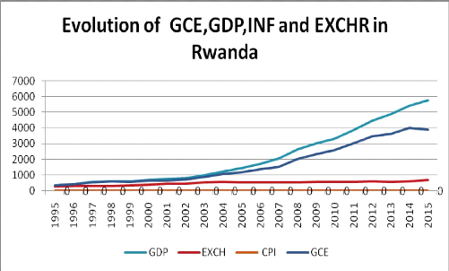
30
Source: World Bank indicators1995-2015 and author's
computation
Figure 2: Status and trends of gross consumption
expenditure, Gross domestic product, Interest rate, Consumer price indices and
exchange rate in Rwanda from 1995 up to 2015
Gross Consumption Expenditure: According to
the above figure, the post 1994 Genocide (from 1995), household consumption in
Rwanda was very low where percentages show that 94.31 % of Rwandans consumed
327.73 Frw. Because of post war period, the economic system were destructed,
infrastructures were ruined by the war so that every economic sector were
shocked. But from 1995, statistics show that there is an increase of the level
of gross consumption expenditure from 1995-2015 where it started from 327.73
Frw from 1995 and grew slowly until 2004 where consumption reached 1056.73.
Within 3 years (from 2005 to 2007), the level of consumption grew quickly where
it reached 1520.55 Frw. Because different initiatives put in economic sector by
the Government of Rwanda, the level of consumption were increased at high rate
where from 2008 to 2011, an increase of 983.67Frw whereby 78% of Rwandans
consumed 3001.55Frw. From that period, the level of consumption grew slowly by
422.6 Frw because of different economic challenges.
31
Gross Domestic Product: According to the
above figure, using the documentary technique, the researcher has obtained data
from the World Bank. The data have been analyzed and
interpreted using the statistical, analytical and synthetic methods. The
statistical method helped the researcher to plot the evolution of GDP of Rwanda
from 1995 to2015. The figure 2 above shows that the gross domestic product has
the upward trends. They are increasing over time because from 1995 up to 2003,
the level of GDP has grown by 656.44 b Frw, but because of economic
reconstruction as well as the whole country, this level grew slowly in a period
of 8years thereafter that period, the level of GDP grew rapidly because after
presidential elections, many policies put in action such as increase of foreign
direct investment, increase of domestic agro processing industries, financing
the small and medium entrepreneurs, etc. Normally, this is shown by the above
given figures where from 2004 up to 2009, there is a high increase compared to
the starting period with 1810.69 b Frw which means that is are positive trend.
From 2010 up to 2015, there is a continuous increase in GDP because the level
of increase is 2417.16 b Frw.
Exchange rate: The exchange rate in Rwanda
has been fluctuated in four main categories under relative period from
1995-2015. From 1995, the Government of Rwanda introduced the regime of
floating exchange rate where this exchange rate is allowed to fluctuate in
response to the economic condition. We normally know that in a fixed exchange
rate regime, the Central Bank trades domestic for foreign currency at a
predetermined level of price. The post Genocide period of 1995-2015 was a
period of reconstruction in whole Country particularly in the economic system.
Therefore, from 1995 up to 1999, the; level of exchange rate has been
fluctuated (increased one hand and decreased on the other hand). The lower
level of net export which is the exports minus imports is the main determinants
of exchange rate. This lower level of net export was low from many years ago
because Rwanda is a landlocked country and it does not have natural resources
that can induce the level of domestic production as well as the level of
export. With policy of monetary targeting used by the central bank of Rwanda,
from 2000 up to 2005, the money market which is introduced in the period of
1999-2005 to increase the level of transactions among domestic commercial
institutions. This has changed many things in Rwandan economic system. The
system faced an increase in money supply where this increase in money causes a
decrease of interest rate of bonds. Because we are in open economy, the
domestic rate of interest would be equal to the world one. So the system faced
many investors who converted Rwandan currency into foreign currency to invest
outside of the Country (Capital outflows). There is therefore a depreciation of
the domestic currency. This depreciation of the domestic currency causes the
exchange rate to flow down, induce the level of net export without forgetting
the level of income. Even if it is so, the national
32
export, at lower level than import, have a lower price outside
the country. The introduction of capital market in Rwanda in 2005 did change
nothing on depreciation of Rwanda currency. From 2005 up to 2011, the exchange
rate continued to decrease where it shifted from 557.82 to 600.31 by one
dollar. Because of the trade balance deficit faced by Rwanda economic system a
longtime ago, there is a continuous decrease of exchange rate which depreciate
our domestic currency whereby from 2012 to 2015, domestic currency depreciated
by 2.81%. Without going far from the facts, an increase in Government spending
(Expansionary fiscal policy) is the only solution because it can increase
income and interest rate on bonds which can make capital inflows and appreciate
the domestic currency. The level of exchange rate will increase which will
lower net export and income. Thus offset occurs between incomes.
Inflation: The annual percentage change in a
Consumer Price Index (Inflation) is used to measure inflation. The Consumer
Price Index (CPI) can be used to index the real value of wages, salaries,
pensions, and price regulation. It is one of the most closely watched national
economic statistics. The consumer price index (CPI) is a statistical estimate
of the level of prices of goods and services bought for consumption by
households. It measures changes in the price level of a market basket of goods
and services used by households. The CPI is calculated by collecting prices of
a sample of representative items over a specific period of time. Goods and
services are divided into categories, sub categories, and sub-indexes. All
information is combined to produce the overall index of consumer expenditures.
Such that the annual percentage change in a CPI is used to measure inflation,
in Rwanda, the level of inflation measured by CPI, from 1996-2002, the levels
of price were decreasing because many people were outside the country due to
the 1994 Genocide while domestic production were high. With many programs of
sensitizing refugees to comeback because of security, the level of population
increased and the level of price started to rise due to lower level of
production.
However, in 1999, a shock happened where the level of price
decreased gradually and it riches a negative value. This was caused by high
level of production (Supply) against lower level of demand. It is like a short
run deflation. From 2003 up to 2008, a continuous rise of price occurred
because of the continuous rise of the population. (DHS: 2005). But again from
2008 to 2015, because many policies put into action by the Government of Rwanda
like, Girinka, Umurenge SACCOs, Agriculture policies of irrigation as well as
new investments in different economic sectors like industrialization, financial
institutions, and so on, all those policies increased the level of consumer
goods therefore the level of price reduced by 12.9% which shows a high impact
in the economy.
33
CPI calculation:
For example, imagine you buy five sandwiches, two magazines,
and two pairs of jeans. In the first period, those goods are market basket at
base period prices = 5(6.00) + 2(4.00) + 2(35.00) = 108.00. Market basket at
current period prices = 5(7.00) + 2(6.00) + 2(45.00) = 137.00. The CPI
represents the cost of a basket of goods and services across the country on a
monthly basis. Those goods and services are broken into eight major groups:
Food and beverages Housing, Apparel, Transportation, Medical care, Recreation,
Education and communication and other goods and services. From the above
example:

From the above figure, the rate of lending interest rate in
Rwanda is at high level. Normally, Rwanda institutions seek for high return
compared to the level of income as well as the rate of people that take credits
in good collaboration with financial institutions to induce the level of
investment in the community. From 1995 to 1999, the rate of lending interest
was 17 and 16%. This is the post Genocide period where financial institutions
started to reconstruct without enough capital as well as qualified employees.
The monetary authorities and commercial banks have had faced the problem of
dealing with the lower level of money. Measures were put in place to call upon
people to use credits as a financial support in order to induce the level of
investment in Rwanda as well as domestic production. Fluctuations continued
where from 2003 to 2009, the level of interest rate changed from 16 to 17%. The
introduction of money market and capital market (1999-2005) has had affected
the increase of that rate. However a continuous depreciation of the domestic
currency affects the level of interest rate because the economic system cannot
attract foreign investors. From 2010 to 2015, the level of interest rate
changed from 18 to 19%. Local people as small and medium entrepreneurs are not
attracted by financial institutions to take loans because of that high level of
interest rate. If is so, the level of investment cannot increase to affect the
level of income. By lower level of income, household consumption is also
decreased.
34
Partial conclusion
With the above findings, the explained variable GCE has upward
trend as it is shown by numbers. By 1995 to 2003, the level of consumption
increased from 327.73 Frw up to 876.37 Frw per household (96.95% to 88.1%) i.e
96.95 % of household in Rwanda consumed 327.73 Frw in 1995, this is the post
1994 Genocide in the country where all sectors including economic ones were
destructed by conflicts. However, after presidential elections, the level of
consumption in Rwanda has gradually increased again because of many policies
put into action by the Government of Rwanda. From 2004 up to 2007, the levelof
consumption faced a high increase because 87.55% up to 73.51% of Rwandan
consumed between 1056.73 Frw to 1520.55 Frw. Thereafter, from 2008 up to 2015,
the level of consumption has been increased by about 2.55% where a decrease
vary between73.51% to 69.4%. Generally, from 1995 up to 2015, the level of
income has affected positively the gross consumption expenditure. The
continuous level of interest rate is a challenge to the household market
basket. The level of inflation is also a challenge to the consumption because
the income from investments is affected by inflation. A continuous depreciation
of the domestic currency to the dollar causes the imported goods to be very
expensive. Therefore, the next chapters give the econometric facts to know the
exact relationship between variables used in the model. Therefore, the
researcher affirms, based on the first hypothesis that the trends of the used
model are upward sloping and the used variables are significantly related.
35
CHAPTER 3: ECONOMETRIC ANALYSIS OF THE RELATIONSHIP
BETWEEN GROSS CONSUMPTION EXPENDITURE AND ITS DETERMINANTS IN
RWANDA
INTRODUCTION
In this chapter, we used econometric method in order to verify
the second provisional answer in the research proposal. To reach targeted
goals, the researcher has developed different point like: introduction to
econometrics, specification of the model, expected sign, data processing, model
estimation and diagnostic tests by using the series collected in the period of
1995 to 2015.
The econometric methodology encompasses the following steps:
+ Statement of the theory
+ Specification of the mathematical model of the theory
+ Specification of the econometrics model
+ Obtaining data
+ Estimation of the parameters of the econometric model
+ Hypothesis testing
+ Forecasting or prediction
+ Use of the model for control of policy purpose
Econometric uses application of mathematical and statistics to
economic data in order to support models
constructed by mathematical economics and obtain numerical
results and to analyze the economic
phenomena. Econometrics quantifies the theoretical phenomena to
test the existence of the relationship
and then specifies exact form. Econometrics begins formulating
econometrics model. In this chapter,
we shall be testing the impact of income, interest rate;
inflation rate and exchange rate on gross
consumption expenditure in Rwanda using econometrics software,
find out economic interpretation on
the data obtained and propose the suggestions and prediction.
3.1 Model specification
The analysis of the economic phenomena is based on some
underlying logical structure known as a model. The model is a simplified
version of the reality: the model describes the behavior of the variables in
the system and it is the basic framework of the analysis. The model is in the
form of equations,
36
composed by dependent variable and independent variables which
are related. The startup of the model is the specification of a mathematical
model. The mathematical model is an equation that expresses relationship
between depend variable and independent variables: changes in dependent
variable are explained 100% by changes occurred in independent variables. Once
the researcher assumed that all changes in dependent variable are not 100%
explained by changes in independent variables, the researcher has added on
mathematical model a term to represent other factors that may have influence on
the dependent variable. The model becomes an econometric model because of this
error term. Normally we don't find a meant relationship among variables that is
why we introduce a disturbance term or error term to represent other factors
that may have influence on dependent variable. The model to be estimated
concerns the determinants affecting aggregate consumption expenditure in
Rwanda. Hence the Gross Consumption Expenditure (GCE) is the dependent variable
and other variables are independent, the GCE is hypothetically assumed to be a
function of consumption of household at current prices.
3.1.1 Hypothesis of the model
Theoretically, macroeconomic references predict that there is
positive correlation between consumption
and income, a negative correlation between consumption and
interest rate a negative correlation between
consumption and inflation and also a negative correlation between
consumption between consumption
and exchange rate. The variables of the model are initially the
consumption function modeled in the
following form:
C=C0+C1Yd
For our case, the gross consumption function is proposed to be
modeled in the following form: GCE:
GCE= P0 +P1GDP+P2INT+P3INF+P4EXR+ut
Where: GCE: The gross consumption expenditure
f30= the intercept
f31, f32, f33 and f34: The coefficients of the model of
coefficients of regression
GDP: The gross domestic product
INT: The lending Interest rate
INF: The inflation rate
EXR: The exchange rate
ut: Error term of t period
37
3.1.2. Expected signs
The expected sign of the slope coefficients in model are:
f30>0, f31>0, f32><0, f33<0, f34<0
f30>0: The intercept (stands for the autonomous
consumption) is positively related to the explained variable GCE and to all
explanatory variables.
f31>: This means that explanatory variable GDP is positively
related to the explained variable GCE.
f32><: This means that the explanatory variable INT is
positively or negatively related to the explained variable GCE.
f33<: Means that the explanatory variable INF is negatively
related to the explained variable GCE.
f34><: Means that the explanatory variable EXCH is
negatively or positively related to the explained variable GCE.
3.1.3 Test and analysis of the data
It is clear that most macroeconomic time series data are not
stationary and are not linear. To make sure that there are all linear, all
variables are transformed into logarithm. In order to avoid obtaining
misleading statistical inferences, the researcher performed the stationarity
test of all variables used in the model.
3.2. Data processing
In this study, we used annual time series data for the period
1995 to2015. Normally, most time series are non-stationary series in the model
and might lead to spurious regressions. The first or the
second difference terms of the most variables will usually be stationary.
3.2.1. Unit root tests
3.2.1.a. Why testing stationarity?
When economic time series are stationary, the application of
Ordinary Least Squares (OLS) estimation is statistically acceptable; and when
they are not stationary, the assumptions upon which OLS
38
Estimation are violated, rendering its application
inappropriate. In this case we use the co-integration test. To test stationary
of all-time series of our model, the E-views 7 software enabled us to use the
test of the Augmented Dickey Fuller (ADF) and Phillips Peron (PP) tests. By
applying the strategy of these tests incorporated in E-views software. Prior to
carrying out a model, it is necessary to examine the time series properties of
the variables included in it. This allows one to determine whether or not the
regression is spurious. For this purpose, stationarity of data set is checked
by using the simple appropriate tests above mentioned. The results of the
stationarity obtained arise as follows in the table:
39
SERIES
|
EQUATION
|
ADF
|
PP
|
CONCLUSION
|
|
lag
|
T-test
|
T-cri
|
Prob
|
T-test
|
T-cri
|
Prob
|
|
LNGCE
|
Intercept
|
0
|
-1.109913
|
-3.020686
|
0.690
|
-1.067673
|
-3.020686
|
0.707
|
LNGCE is not
stationary at level
|
|
Trend& Intercept
|
0
|
-1.480747
|
-3.658446
|
0.801
|
-11.710319
|
-3.658446
|
0.708
|
|
None
|
0
|
5.932190
|
-1.959071
|
1.000
|
5.932190
|
-1.959071
|
1.000
|
|
LNGDP
|
Intercept
|
1
|
-0.479496
|
-3.029970
|
0.875
|
-0.887935
|
-3.020686
|
0.770
|
LNGDP is not
stationary at level
|
|
Trend& Intercept
|
3
|
-3.350081*
|
-3.710782
|
0.091
|
-1.654032
|
-3.658446
|
0.733
|
|
None
|
1
|
1.967458**
|
-1.960171
|
0.984
|
6.832295** *
|
-1.969071
|
1.000
|
|
INT
|
Intercept
|
0
|
-0.240037
|
-3.020686
|
0.918
|
-0.059694
|
-3.020686
|
0.941
|
INT is not stationary at level
|
|
Trend& Intercept
|
1
|
-3.157576
|
-3.673616
|
0.122
|
-3.639768*
|
-3.658446
|
0.051
|
|
None
|
0
|
1.012776
|
-1.959071
|
0.911
|
1.231349
|
-1.959071
|
0.938
|
|
INF
|
Intercept
|
0
|
-2.822727*
|
-3.020686
|
0.072
|
-2.743902*
|
-3.020686
|
0.084
|
INF is not stationary at level
|
|
Trend& Intercept
|
0
|
-2.747607
|
-3.658446
|
0.230
|
-2.680366
|
-3.658446
|
0.253
|
|
None
|
0
|
-1.522258
|
-1.959071
|
0.117
|
-1.442881
|
-1.959071
|
0.134
|
|
LNEXCH
|
Intercept
|
0
|
-2.120302
|
-3.020686
|
0.239
|
-3.120302
|
-3.020686
|
0.239
|
LNEXCH is not
stationary at level
|
|
Trend& Intercept
|
3
|
-2.405621
|
-3.710482
|
0.363
|
-1.700882
|
-3.658446
|
0.712
|
|
None
|
1
|
1.745474*
|
-1.960171
|
0.975
|
2.823701
|
-1.959071
|
0.997
|
Source: World Bank indicators1995-2015 and author's computation
Table 2: Stationarity at Level
40
SERIES
|
EQUATION
|
ADF
|
PP
|
CONCLUSION
|
|
lag
|
T-test
|
T-cri
|
Prob
|
T-test
|
T-cri
|
Prob
|
|
LNGCE
|
Intercept
|
0
|
-3.201338**
|
-3.029970l
|
0.035
|
-3.147755
|
-3.029970
|
0.039
|
LNGCE is not
stationary at first
difference
|
|
Trend& Intercept
|
0
|
-3.170959
|
-3.676316
|
0.119
|
-3.140534
|
-3.673616
|
0.125
|
|
None
|
1
|
-1.883162*
|
-1.961409
|
0.058
|
-1.783670*
|
-1.96071
|
0.073
|
|
LNGDP
|
Intercept
|
0
|
-2.698763*
|
-3.029970
|
0.092
|
-2.621696
|
-3.029970
|
0.106
|
LNGDP is not
stationary at first
difference
|
|
Trend& Intercept
|
0
|
-2.634522
|
-3.676316
|
0.270
|
-2.570212
|
-3.673616
|
0.295
|
|
None
|
0
|
-1.500754
|
-1.960171
|
0.121
|
-1.460394
|
-1.960171
|
0.130
|
|
INT
|
Intercept
|
1
|
-4.739894***
|
-3.040391
|
0.001
|
-5.966575***
|
-3.029970
|
0.000
|
INT is stationary at first difference
|
|
Trend& Intercept
|
1
|
-4.740442**
|
-3.690814
|
0.007
|
-6.311193***
|
-3.673616
|
0.000
|
|
None
|
0
|
-3.706693***
|
-1.960171
|
0.000
|
-3.704162***
|
-1.960171
|
0.000
|
|
INF
|
Intercept
|
0
|
-4.942504***
|
-3.029970
|
0.001
|
-8.562930***
|
-3.029970
|
0.000
|
INF is stationary at first difference
|
|
Trend& Intercept
|
1
|
-4.880297***
|
-3.690814
|
0.005
|
-8.930822***
|
-3.673616
|
0.000
|
|
None
|
0
|
-5.067116***
|
-1.960171
|
0.000
|
-8.255686***
|
-1.960171
|
0.000
|
|
LNEXCH
|
Intercept
|
3
|
-1.482842
|
-3.065585
|
0.516
|
-3.071608**
|
-3.029970
|
0.046
|
LNECH is not
stationary at first
difference
|
|
Trend& Intercept
|
3
|
-1.531298
|
-3.733200
|
0.774
|
-2.637027
|
-3.673616
|
0.269
|
|
None
|
0
|
-2.354457**
|
-1.960171
|
0.021
|
-2.354457**
|
-1.960171
|
0.021
|
Source: World Bank indicators1995-2015 and author's computation
Table 3: Stationarity at first difference
41
SERIES
|
EQUATION
|
ADF
|
PP
|
CONCLUSION
|
|
lag
|
T-test
|
T-cri
|
Prob
|
T-test
|
T-cri
|
Prob
|
|
LNGCE
|
Intercept
|
1
|
-6.094004***
|
-3.040391
|
0.000
|
-6.381671***
|
-3.040391
|
0.000
|
LNGCE is
stationary at
second difference
|
|
Trend& Intercept
|
2
|
-3.708039*
|
-3.733200
|
0.042
|
-6.153897***
|
-3690814
|
0.000
|
|
None
|
0
|
-6.123911***
|
-1.961409
|
0.000
|
-6.388171***
|
-1.961409
|
0.000
|
|
LNGDP
|
Intercept
|
0
|
-4.676807***
|
-3.040391
|
0.001
|
-4.831284***
|
-3.040391
|
0.001
|
LNGDP is
stationary at
second difference
|
|
Trend& Intercept
|
1
|
-4.729190**
|
-3.710482
|
0.008
|
-4.610669**
|
-3.690814
|
0.009
|
|
None
|
0
|
-4.709419***
|
-1.961409
|
0.000
|
-4.873309***
|
-1.961409
|
0.000
|
|
INT
|
Intercept
|
2
|
-5.474011***
|
-3.065585
|
0.000
|
-7.841476***
|
-3.040391
|
0.000
|
INT is stationary
at second
difference
|
|
Trend& Intercept
|
2
|
-5.202147***
|
-3.733200
|
0.004
|
-9.109500***
|
-3.690814
|
0.000
|
|
None
|
2
|
-5.738162***
|
-1.964418
|
0.000
|
-7.932883***
|
-1.961409
|
0.000
|
|
INF
|
Intercept
|
2
|
-5.472188***
|
-3.065585
|
0.000
|
-14.57497***
|
-3.040391
|
0.000
|
INF is stationary
at second
difference
|
|
Trend &
Intercept
|
2
|
-5.570167***
|
-3733200
|
0.002
|
-13.16833***
|
-3.690814
|
0.000
|
|
None
|
2
|
-5.688618***
|
-1.964418
|
0.000
|
-14.48986***
|
-1.961409
|
0.000
|
|
LNEXCH
|
Intercept
|
3
|
-2.356842
|
-3.081002
|
0.048
|
-5.010709***
|
-3.040391
|
0.001
|
LNESCH is stationary at second difference
|
|
Trend& Intercept
|
3
|
-2.407857
|
-3.759743
|
0.361
|
-4.836133**
|
-3.690814
|
0.006
|
|
None
|
3
|
-2.402642**
|
-1.966270
|
0.020
|
-5.203143***
|
-1.961409
|
0.000
|
Source: World Bank indicators1995-2015 and author's computation
Table 4: Stationarity at second difference
3.2.1.b. Interpretation of stationarity test
From the above table, the so called stars:
***: Stationary at 1% level of significance
**: stationary at 5% level of significance *:
Stationary at 10 % level of significance
- LNGCE is not stationary at both level but
it becomes stationary at second difference at 1% level of significance, when we
consider all equations.
- LNGDP is not stationary at both level and
first difference but it becomes stationary at second difference when we
consider all equations.
- INT is not stationary at level but it
becomes stationary at both first and second difference when we consider all
equations.
- INF is not stationary at level but it is
stationary at both first and second difference when we consider all equations
using.
- LNEXCH is not stationary at level but it
becomes stationary at first difference when we consider none by all equations
and it is stationary at second difference when we consider all equations. Our
model meets the condition for co-integration because all other series are
integrated of the same order after being differentiated.
3.3 Estimation of long run model 3.3.1 Co-integration
test
Co-integration is a statistical property of a collection of
time series variables X1, X2... Xk. First, all of the series must be integrated
of order 1, second, if a linear combination of this collection is integrated of
order zero, then the collection is said to be co-integrated. With Johansen
approach, we use trace and Maximum Eigenvalue tests to justify co-integration.
If two or more series are themselves non-stationary but a linear combination of
them is stationary, the series are said to be co-integrated. (KASAI,
2009:43).
54
Date: 08/12/16 Time: 12:59
Sample (adjusted): 1997 2015
Included observations: 19 after adjustments Trend assumption:
Linear deterministic trend Series: LNGCE LNGDP INT INF LNEXCHR
Lags interval (in first differences): 1 to 1
Unrestricted Co-integration Rank Test (Trace)
Hypothesize
d Trace 0.05
Critical
No. of CE(s) Eigenvalue Statistic Value Prob.**
|
None *
|
0.986335
|
149.9639
|
69.81889
|
0.0000
|
|
At most 1 *
|
0.862347
|
68.39784
|
47.85613
|
0.0002
|
|
At most 2 *
|
0.614846
|
30.72045
|
29.79707
|
0.0390
|
|
At most 3
|
0.446337
|
12.59231
|
15.49471
|
0.1306
|
|
At most 4
|
0.069054
|
1.359523
|
3.841466
|
0.2436
|
Trace test indicates 3 co-integrating eqn(s) at the 0.05 level *
denotes rejection of the hypothesis at the 0.05 level **MacKinnon-Haug-Michelis
(1999) p-values
Unrestricted Co-integration Rank Test (Maximum Eigenvalue)
Hypothesize
d Max-Eigen 0.05
Critical
No. of CE(s) Eigenvalue Statistic Value Prob.**
|
None *
|
0.986335
|
81.56606
|
33.87687
|
0.0000
|
|
At most 1 *
|
0.862347
|
37.67739
|
27.58434
|
0.0018
|
|
At most 2
|
0.614846
|
18.12814
|
21.13162
|
0.1251
|
|
At most 3
|
0.446337
|
11.23279
|
14.26460
|
0.1429
|
|
At most 4
|
0.069054
|
1.359523
|
3.841466
|
0.2436
|
55
Max-eigenvalue test indicates 2 co-integrating eqn(s) at the 0.05
level
* denotes rejection of the hypothesis at the 0.05 level
**MacKinnon-Haug-Michelis (1999) p-values
Unrestricted Co-integrating Coefficients (normalized by
b'*S11*b=I):
|
LNGCE
|
LNGDP
|
INT
|
INF
|
LNEXCHR
|
|
42.28232
|
-30.85109
|
-4.837431
|
0.013107
|
-4.937743
|
|
0.717548
|
-3.422595
|
1.791842
|
0.614326
|
3.563539
|
|
2.098782
|
-3.153853
|
-0.823262
|
-0.111838
|
8.181454
|
|
-26.75212
|
25.13077
|
-0.712632
|
0.155683
|
-3.249637
|
|
-20.33113
|
20.86315
|
-0.252021
|
0.018610
|
-3.100465
|
Source: World Bank indicators1995-2015 and author's computation
Table 5: Long run Johansen Co-integration test output
3.3.2 Interpretation of Johansen Co-integration test
output
Trace test indicates 3 co-integrating eqn(s) at the 0.05 level
and the
Max-eigenvalue test indicates 2 co-integrating eqn(s) at the 0.05
level
From these findings, the researcher concluded that variables have
a long run relationship.
56
3.3.3 Long run output
Dependent Variable: LNGCE Method: Least Squares
Date: 08/11/16 Time: 20:33 Sample: 1995 2015
Included observations: 21
Variable Coefficient Std. Error t-Statistic Prob.
LNGDP 0.867339 0.032528 26.66452
0.0000
INT -0.032394 0.019717 1.642904
0.0499
INF -0.040527 0.002049 0.257232
0.0303
LNEXCHR -0.025767 0.065889 -0.391066
0.0409
C 0.371652 0.394843 0.941266
0.3606
R-squared 0.998411 Mean dependent var
7.124936
Adjusted R-squared 0.998014 S.D. dependent var
0.812793
S.E. of regression 0.036223 Akaike info criterion -3.593979
Sum squared resid 0.020994 Schwarz criterion -3.345284
Log likelihood 42.73678 Hannan-Quinn criter. -3.540006
F-statistic 2513.431 Durbin-Watson stat 1.347986
Prob(F-statistic) 0.000000
Source: World Bank indicators1995-2015 and author's
computation
Table 6: Long run output effect of changes in GDP,
INT, INF, and EXCHR on Gross Consumption Expenditure
3.3.3.1 Interpretation of the long run Model
From the above table, results given by Eviews8 highlight the
follows:
LNGCE=
0.371652+0.867339LNGDP-0.032394INT-0.040527INF-0.025767LNEXCHR
? From the above output of long run equation, first, the gross
domestic product (GDP) is positively related to gross consumption expenditure
(GCE) as expected in theory. This means that, when GDP increases by one more
units, GCE increases by 86% by considering other variables constant. (Ceteris
paribus)
57
? Second, from the above table, the interest rate is
negatively related to GCE which means that: increases by one more units in
interest rate, decreases gross consumption expenditure (GCE) by 3.2%, ceteris
paribus.
? Third, from our findings, the inflation rate is negatively
related to GCE which means that: an increase by one more units in inflation
rate decreases the GCE by 4.0% ceteris paribus.
? Fourth, from our findings, the exchange rate is negatively
related to GCE which means that: an increase by one more unit in exchange rate
(depreciation) decreases the GCE by 2.5% ceteris paribus.
The probabilities of coefficients show that all explanatory
variables except that of the constant, are statistically significant because
they are less than 0.05 or less than 5%.
The coefficient of Determination R-squared (R2)
equals 99.8% indicates that the explanatory variables contribute significantly
in explaining gross consumption expenditure. This is the indicator of a well
fitted model. The Prob (F-statistic) of 0.0000
allow us to reject the null hypothesis which states that all
explanatory variables do not collectively explain the explained variable and
therefore all explanatory variables collectively influence the gross
consumption expenditure.
3.3.4. Vector Auto-regression Estimates (Short run
relationship) The system equation for the short run is:
Equation: LNGCE = C(1)*LNGCE(-1) + C(2)*LNGCE(-2) +
C(3)*LNGDP(-1)
+ C(4)*LNGDP(-2) + C(5)*INT(-1) + C(6)*INT(-2) + C(7)*INF(-1) +
C(8)
*INF(-2) + C(9)*LNEXCH(-1) + C(10)*LNEXCH(-2) +
|
C(11)
Observations: 19
|
|
|
|
|
R-squared
|
0.994725
|
Mean dependent var
|
7.254886
|
|
Adjusted R-squared
|
0.988131
|
S.D. dependent var
|
0.738783
|
|
S.E. of regression
|
0.080487
|
Sum squared resid
|
0.051826
|
|
Durbin-Watson stat
|
1.816104
|
|
|
Source: World Bank indicators1995-2015 and author's
computation
Table 7: Short run relationship effect of changes in GDP,
INT, INF, and EXCHR on Gross Consumption Expenditure
58
3.3.4.1. Interpretation of the short run equation and the
coefficients of probabilities
From the above findings, the probability except C (1)
and (C3) shows that individually, explanatory
variables are not statistically significant to influence the dependent variable
because they are greater than 5% level of significance except
the GDP which has a probability of 4.1%. From the above
results obtained from E-views8 software, not all conditions of a good model are
observed:
- The coefficients are different from zero which is good for the
model
- The coefficient (C1) of residuals is positive.
The determination R-squared (R2) is greater than
99.4% which also good for the model and from the output coefficients are not
statistically significant to influence the dependent variable except the GDP.
This is because their probabilities are greater than 5% level of significance
except that of GDP which is 4.1% and this means that these independent
variables are not significant to influence gross consumption expenditure in the
short run.
3.4 Diagnostic tests
After testing the short run equation, the supplementary tests
are necessary to verify if the hypothesis of classical regression are
confirmed.
3.4.1 Jarque-bera test (Normality test)
The result of this test arises on the below mentioned graph:
Series: Residuals
Sample 1995 2015
Observations 21
|
Mean Median Maximum
Minimum
Skewness
Kurtosis
Jarque-Bera
Probability
|
|
|
6 5 4 3 2
1 0
|
|
|
-0.06 -0.04 -0.02 0.00 0.02 0.04
|
Source: World Bank indicators1995-2015 and author's
computation. Figure 3: Jarque-bera Test output
59
The assumptions of these tests are below mentioned:
H0 (Null hypothesis): The residuals are normally
distributed
Std. Dev.
H1 (The alternative hypothesis): The residuals are not
normally distributed.
The null hypothesis is not rejected because the probability of
33% is greater than 10%.
The null hypothesis is not rejected means that residuals are
normally distributed.
60
3.4.2 Breusch-Godfrey test (Serial correlation LM test) The
E-views 8 estimation output is the following:
Breusch-Godfrey Serial Correlation LM Test:
F-statistic 0.424899 Prob. F(2,14) 0.6620
Obs*R-squared 1.201752 Prob. Chi-Square(2) 0.5483
Source: World Bank indicators1995-2015 and author's computation
Table 8: Serial correlation tests
The assumptions for this test are the following: H0: no serial
correlation (errors are not correlated). H1: There is serial correlation.
The null hypothesis is not rejected when the probability is less
than 10%.
The probability of obs* R-squared is 54% greater than 10% which
means that the model has not the errors of residuals autocorrelation.
3.4.3 Heteroscedasticity Test (Breusch Pagan Godfrey)
Heteroscedasticity Test: Breusch-Pagan-Godfrey
|
F-statistic
|
0.135075
|
Prob. F(4,16)
|
0.9670
|
|
Obs*R-squared
|
0.685978
|
Prob. Chi-Square(4)
|
0.9530
|
|
Scaled explained SS
|
0.308383
|
Prob. Chi-Square(4)
|
0.9893
|
Source: World Bank indicators1995-2015 and author's computation.
Table 9: Heteroscedasticity Test
The assumptions for this test are the following: Ho: the model is
not homoscedastic
H1: the model is heteroscedastic
61
The probability of Scaled explained SS (Chi- square) 98% is
greater than 10% level of significance which means that the model is
homoscedastic.
3.5 Stability tests
3.5.1 Ramsey reset test
The test above mentioned indicates whether the model is well
specified or not. The assumptions for this test are as follows;
H0= the model is specific.
H1= the model is not specific.
Ramsey RESET Test Equation: UNTITLED
Specification: LNGCE LNGDP INT INF LNEXCH C
Omitted Variables: Squares of fitted values
|
Value
|
df
|
Probability
|
|
t-statistic
|
1.271153
|
15
|
0.2230
|
|
F-statistic
|
1.615829
|
(1, 15)
|
0.2230
|
|
Likelihood ratio
|
2.148417
|
1
|
0.1427
|
Source: World Bank indicators1995-2015 and author's computation
Table 10: Ramsey reset Test
From the above finding, the probability of 22% is greater than
10% level of significance which means that we accept the null hypothesis
therefore the specification of the model is
good.in other words, the model is BLUE (
Best Linear Unbiased Estimator).
3.5.2 Recursive estimates (OLS only): Cusum test
With CUSUM test, the pace of the graph shows that the parameters
of this model are stable when it is noticed that the representative curve is
located between the two lines indicating the critical point of 10% level of
significance. If it is not so, parameters are said to be unstable.
62
12 8 4 0
-4 -8 -12
00 01 02 03 04 05 06 07 08 09 10 11 12 13 14 15
Source: World Bank indicators1995-2015 and author's computation
Figure 4: Cusum test
CUSUM 5% Significance
The graph shows that the parameters are stable because the
shape of the curve is (shape in blue color) between
two critical points.
Partial conclusion
This chapter was aimed to verify the impact of National income
(GDP), interest rate, inflation rate and exchange rate on gross consumption
expenditure in Rwanda. To achieve our goal, we have chosen different
econometric tests, the unit root test shows used variables are not stationary
at both level and stationary first difference but they are stationary at second
difference. We have undertaken co-integration test and estimate long and short
run equation. After estimation, the researcher has realized that in the
long-run analysis, GDP are related positively to the GCE. All coefficients
independent variables are statistically significant at 5% level of reference,
in long-run. R-squared equals 99.8% and Adjusted R-squared equals 99%, show the
goodness-of-fit of estimated model. Up to 99.2% of long-run fluctuations in GCE
are influenced by changes GDP. By these findings, the researcher affirms the
second hypothesis above verified stated that there is statistical significant
relationship between GCE and its associates in Rwanda. According to the result
of diagnostic test, that the model is good and respects the classical
assumption of homoscedasticity, no autocorrelation of errors and no serial
correlation as well, there is
63
normality of residuals and stability of parameters. The
researcher also noted that the model is stable. Therefore, the researchers
affirm the second hypothesis that there is a long run relationship between
gross consumption expenditure and its associates in Rwanda from1995-2015.
64
GENERAL CONCLUSION AND SUGGESTIONS
From the above output of long run equation, one, the gross
domestic product (GDP) is positively related to gross consumption expenditure
(GCE) as expected in theory. This means that, when GDP increases by one more
units, GCE increases by 86% by considering other variables constant. (Ceteris
paribus)
Two, the interest rate is negatively related to GCE which
means that: increases by one more units in interest rate, decreases gross
consumption expenditure (GCE) by 3.2%, ceteris paribus. This is because the
higher the interest, the lower the investment and this discourages
consumption.
Three, from the findings, the inflation rate is negatively
related to GCE which means that an increase by one more units in inflation rate
decreases the GCE by 4.0% ceteris paribus. This is because a continuous rise in
prices reduces the level of consumption expenditure.
Four, the exchange rate is negatively related to GCE which
means that: an increase by one more units in exchange rate (depreciation)
decreases the GCE by 2.5% ceteris paribus. Rwanda like other developing
countries depends much on imports and this shows how the demand for the foreign
currency ($) is always high compared to the demand of the local currency. The
level of export like Tea, and Coffee is very low and its price is also low
compared to foreign export on international market. Therefore the Government
has to intervene with its reserves to cover this deficit therefore the
wellbeing of the community can be enhanced in Rwanda.
SUGGESTIONS
If Rwanda wants to induce its level of economy, maintain the
wellbeing of people and become more competitive in order to participate in
international trade, the following should be done:
V' Policymakers in Rwanda should strengthen efforts
to control the rate of inflation in order to become more competitive in durable
way. This can be achieved if internal as well as external sources of inflation
are addressed.
V' Rwanda should continue to encourage capital
inflows and investments from local investors as well as foreign investors.
Investors are revenues from capital inflows should be oriented in sectors where
Rwanda has comparative advantages by insisting on sectors which can allow the
country to increase exports and improve its competitiveness in international
markets. For sure, the increase and a good management of those investments can
help the country firms to enjoy economies of
65
scale and their advantages. This will help the country to
increase its level of domestic production and the welfare of the community.
V' Rwanda is advised to continue to encourage
investments and orient them in technological use and that technology should be
used in strategic sectors able to increase the Rwanda production and export as
well. The technological use also can allow the country to produce more and to
export products with increased value. This high level of production will reduce
the level of unemployment which is at high level and will reduce the external
dependency as well.
V' As openness has been found to bring effects on
Rwandan competitiveness in international trade while closeness brings negative
effects on it, Rwanda is advised to continue its movement of reducing trade
barriers in international trade. This can be done by supporting the idea of
economic integration but via increment of production in quality and quantity as
well as the cheapest ways of connecting the country with other countries should
be a priority. Economic authorities must sensitize people to participate in
economic integration and expand the market. Rwanda is advised to look forward
rapid economic growth to middle income status via implementing development
policies, increase poverty reduction measures, enhance private sector as engine
of growth via increasing youth entrepreneurship and job creation therefore the
welfare can be consistent.
66
REFERENCES
(A) Books
· A.C Pigou (1932): `The economics of welfare' Macmillan
and Co., 4th edition, London, UK.
· ASSIMWE M. K (2009),»Fundamental Economics»2
nd edition.
· Blanchard O. (2003): `Macroeconomics»,
3rd edition, USA.
· Blanchard Olivier and Cohen Daniel
(2006):'Macroeconomics'4th edition, Paris
· Christopher D. C. (2016) `Two-Period Optimal Consumption
Problem': 2Period LC Model
· Fisher, Irving (1930): `The Theory of Interest'.
MacMillan, New York.
· Fisher, Irving (1930): The Theory of Interest. MacMillan,
New York.
· Froyen T. Richard(2005):'Macroeconomics Theories and
policies,8th edition, USA
· J.B.F Belong (2002): Macroeconomic 2nd
edition.
· John Maynard K. (1936) `The general theory of Employment,
Interest rate and Money' 1st edition, UK.
· Marshall A (1890), `Principle of economics' London,
UK.
· Milton Friedman (2008) `Theory of the Consumption
Function' Princeton University Press and copyrighted: USA.
· Newbold, P. (1977)' the time series approach to
econometric model building» in new method on business cycle research:
Proceedings from a conference, edited by C.A Sims Federal Reserve Bank of
Minneapolis.
· Ramathan, R. (1992) «, Introductory Econometrics
with Applications» Second Edition. Hartcout New York, Brace Javanovic.
· Samuelson, Paul A (1937): «A note on measurement of
utility,» The Review of Economic Studies, 4(2), 155-161
(B) Journals
· Granger C. W.J (1997)' Modeling the long run in Applied
Economics' Economic Journal: Cambridge University Press.
· Pablo Cotler and Deyanira A. (2013) The Business and
Economics Research Journal: Volume 6, Issue 1, 2013, 69-81, Brighton, UK.
67
(C) Reports
· Enquete Integrale sur les conditions de vies des
ménages (ECV): Kigali, National Institute of Statistics of Rwanda.
· NISR (2012)' The Fourth population and housing
Census», Rwanda Retrieved February, 26, 2015: From National Institute of
Statistics of Rwanda.
· NISR (2014) `Indicators of Agriculture Share on
GDP», Kigali- Rwanda.
· NISR (2014) `Statistical Year Book' 2014, Kigali:
National Statistics of Rwanda.
· NISR (2015a): Main Indicators report. `Integrated
Household Living Conditions Survey'
· NISR (2015b) Rwanda Poverty Profile 2013-2014 `Results of
Integrated Household living Conditions Survey', Kigali, National Institute of
Statistics of Rwanda.
· NISR(2015) `Industries' contribution to the Rwandan
Economy', Kigali-Rwanda
· REMA (2013) `State of environment and outlook
report», Kigali.
· REMA (2015) `A toolkit for the development of smart green
villages in Rwanda', Kigali.
· UNDESA (2014) Country profile, Rwanda:» Retrieved
May 16, 2015, From United Nations, department of economic and social
affairs» population division, (2014): World Urbanization prospect.
(D) Unpublished
· U.L.K (2016) `Handout of macroeconomics, Year 3': Kigali
Campus
· World Bank (2014a) `Support to Rwanda Transformation of
Agriculture sector Program Phase3-Program-for-Results (P148927), Environmental
and social systems assessment (ESSA). The World Bank Group.
· World Bank (2014b) `Rwanda Economic Update', edition
No 6, Unearthing the Subsoil Mining and its contribution to National
Development: The World Bank Group..
(E) Electronic Sources
·
Www.
dataset.coordination@ons.gsi.gov.uk
68
APPENDICES
69
APPENDICES I
Vector Auto-regression Estimates
Date: 08/12/16 Time: 20:50
Sample (adjusted): 1997 2015
Included observations: 19 after adjustments
Standard errors in ( ) & t-statistics in [ ]
LNGCE LNGDP INT INF LNEXCH
LNGCE(-1) 0.899273 -0.935539 3.357366 -69.72302 0.419394
(0.84695) (0.47771) (2.69818) (30.6650) (0.46412)
[-1.06178] [-1.95840] [ 1.24431] [-2.27370] [ 0.90363]
LNGCE(-2) -0.617865 -1.231620 3.074383 -21.55429 -0.277260
(0.94943) (0.53551) (3.02465) (34.3754) (0.52028)
[-0.65078] [-2.29991] [ 1.01644] [-0.62703] [-0.53291]
LNGDP(-1) 2.170781 2.036976 0.545987 112.6920 -0.467200
(1.08084) (0.60963) (3.44331) (39.1335) (0.59229)
[ 2.00842] [ 3.34134] [ 0.15856] [ 2.87968] [-0.78880]
LNGDP(-2) 0.089172 0.617072 -4.684257 -41.62889 0.427809
(1.21598) (0.68585) (3.87382) (44.0263) (0.66635)
[-0.07333] [ 0.89972] [-1.20921] [-0.94555] [ 0.64202]
INT(-1) 0.130199 0.133022 0.178025 7.127216 -0.048968
(0.08519) (0.04805) (0.27141) (3.08459) (0.04669)
[ 1.52826] [ 2.76827] [ 0.65593] [ 2.31058] [-1.04888]
INT(-2) -0.014810 0.038596 -0.440924 -1.075148 -0.021684
(0.06972) (0.03932) (0.22210) (2.52415) (0.03820)
[-0.21244] [ 0.98155] [-1.98527] [-0.42594] [-0.56759]
INF(-1) -0.007165 -0.006390 -0.053345 -0.569278 -0.006710
(0.01031) (0.00581) (0.03284) (0.37321) (0.00565)
[-0.69511] [-1.09902] [-1.62447] [-1.52537] [-1.18786]
INF(-2) -0.001416 0.001014 0.029837 -0.146464 -0.004654
(0.00684) (0.00386) (0.02180) (0.24776) (0.00375)
[-0.20697] [ 0.26263] [ 1.36865] [-0.59115] [-1.24111]
LNEXCH(-1) -0.000271 -0.039869 1.475965 -7.739846 0.924791
(0.51597) (0.29103) (1.64377) (18.6816) (0.28275)
[ 0.00053] [-0.13700] [ 0.89791] [-0.41430] [ 3.27071]
LNEXCH(-2) 0.123371 0.357768 -2.060134 20.95787 -0.021807
70
|
(0.56873)
|
(0.32078)
|
(1.81185)
|
(20.5919)
|
(0.31166)
|
|
[ 0.21692]
|
[ 1.11529]
|
[-1.13703]
|
[ 1.01777]
|
[-0.06997]
|
|
C
|
0.034490
|
-1.478500
|
9.862714
|
-53.04916
|
1.245924
|
|
(1.32734)
|
(0.74866)
|
(4.22861)
|
(48.0585)
|
(0.72737)
|
|
[ 0.02598]
|
[-1.97485]
|
[ 2.33238]
|
[-1.10385]
|
[ 1.71291]
|
|
R-squared
|
0.994725
|
0.998666
|
0.972631
|
0.801377
|
0.985683
|
|
Adj. R-squared
|
0.988131
|
0.996999
|
0.938419
|
0.553098
|
0.967786
|
|
Sum sq. resids
|
0.051826
|
0.016487
|
0.525985
|
67.93888
|
0.015563
|
|
S.E. equation
|
0.080487
|
0.045397
|
0.256414
|
2.914166
|
0.044106
|
|
F-statistic
|
150.8530
|
599.0038
|
28.42987
|
3.227731
|
55.07711
|
|
Log likelihood
|
29.13108
|
40.01133
|
7.115920
|
-39.06444
|
40.55951
|
|
Akaike AIC
|
-1.908535
|
-3.053824
|
0.408851
|
5.269941
|
-3.111527
|
|
Schwarz SC
|
-1.361754
|
-2.507044
|
0.955631
|
5.816722
|
-2.564747
|
|
Mean dependent
|
7.254886
|
7.458007
|
17.54053
|
6.294737
|
6.225143
|
|
S.D. dependent
|
0.738783
|
0.828705
|
1.033282
|
4.359214
|
0.245744
|
|
Determinant resid covariance (dof
|
|
|
adj.)
|
6.99E-11
|
|
Determinant resid covariance
|
9.25E-13
|
|
Log likelihood
|
128.4321
|
|
Akaike information criterion
|
-7.729693
|
|
Schwarz criterion
|
-4.995790
|
System: UNTITLED
Estimation Method: Least Squares Date: 08/11/16 Time: 20:44
Sample: 1997 2015
|
Included observations: 19
Total system (balanced) observations 95
|
|
|
|
Coefficient
|
Std. Error
|
t-Statistic
|
Prob.
|
C(1)
|
-0.899257
|
0.846944
|
-1.061766
|
0.2947
|
C(2)
|
-0.617883
|
0.949425
|
-0.650798
|
0.5189
|
C(3)
|
2.170760
|
1.080837
|
2.008406
|
0.0414
|
C(4)
|
-0.089151
|
1.215976
|
-0.073317
|
0.9419
|
C(5)
|
0.130199
|
0.085195
|
1.528257
|
0.1343
|
C(6)
|
-0.014809
|
0.069715
|
-0.212417
|
0.8329
|
C(7)
|
-0.007165
|
0.010308
|
-0.695113
|
0.4910
|
C(8)
|
-0.001416
|
0.006843
|
-0.206958
|
0.8371
|
C(9)
|
0.000271
|
0.515974
|
0.000525
|
0.9996
|
C(10)
|
0.123375
|
0.568734
|
0.216929
|
0.8294
|
C(11)
|
|
0.034467
|
1.327341
|
0.025967
|
0.9794
|
|
Source: World Bank indicators1995-2015 and author's
computation
71
APPENDICES II
Effects of changes in GDP, interest rate, inflation and
exchange rate on gross consumption
expenditure in Rwanda
Co-integration test
Date: 08/11/16 Time: 20:24
Sample (adjusted): 1997 2015
Included observations: 19 after adjustments
Trend assumption: Linear deterministic trend
Series: LNGCE LNGDP INT INF
LNEXCH
Lags interval (in first differences): 1 to 1
Unrestricted Co-integration Rank Test (Trace)
|
Hypothesized No. of CE(s)
|
Eigenvalue
|
Trace
Statistic
|
0.05
Critical Value
|
Prob.**
|
|
None *
|
0.986335
|
149.9639
|
69.81889
|
0.0000
|
|
At most 1 *
|
0.862347
|
68.39784
|
47.85613
|
0.0002
|
|
At most 2 *
|
0.614846
|
30.72045
|
29.79707
|
0.0390
|
|
At most 3
|
0.446337
|
12.59231
|
15.49471
|
0.1306
|
|
At most 4
|
0.069054
|
1.359523
|
3.841466
|
0.2436
|
Trace test indicates 3 co-integrating eqn(s) at the 0.05 level *
denotes rejection of the hypothesis at the 0.05 level **MacKinnon-Haug-Michelis
(1999) p-values
Unrestricted Co-integration Rank Test (Maximum Eigenvalue)
|
Hypothesized No. of CE(s)
|
Eigenvalue
|
Max-Eigen
Statistic
|
0.05
Critical Value
|
Prob.**
|
|
None *
|
0.986335
|
81.56606
|
33.87687
|
0.0000
|
|
At most 1 *
|
0.862347
|
37.67739
|
27.58434
|
0.0018
|
|
At most 2
|
0.614846
|
18.12814
|
21.13162
|
0.1251
|
|
At most 3
|
0.446337
|
11.23279
|
14.26460
|
0.1429
|
|
At most 4
|
0.069054
|
1.359523
|
3.841466
|
0.2436
|
Max-eigenvalue test indicates 2 co-integrating eqn(s) at the 0.05
level * denotes rejection of the hypothesis at the 0.05 level
**MacKinnon-Haug-Michelis (1999) p-values
Source: World Bank indicators1995-2015 and author's
computation


