Machine learning for big data in galactic archaeology

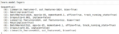
2.2 Linear regression with fast.ai

To begin our machine learning project and create our first neural network we decided to use fast.ai, a package based on the Python module PyTorch and created to simplify the creation and training of neural networks and so to make it accessible for everyone no matter the domain of application. It was founded by researcher Jeremy Howard and AI expert Rachel Thomas. Together they published 14 video courses of about 2 hours each for making fast.ai clear and understandable to anyone having basic notions of Python.

The first step of this internship consisted of taking those courses to get comfortable with machine learning vocabulary and with fast.ai. To test it on a close but simplified situation, a linear regression solving net was created, based on Equation 2.2.1:

y = a1 x1 + a2 · x2 + a3 · x3 + a4 · x4 + a5 · x5 + a6 · x6 + a7 · x7 (2.2.1)

where {x1,...,x7} were the inputs, created randomly to correspond approximately to our photometric data, {a1,...,a7} were coefficients and y was the output, corresponding to the value of metallicty expected for the object. The ai coefficients were chosen arbitrarily to create artificially links between the inputs and the output, as it is the case in our real data. Our dataset is thus a huge table of size N x 8, N being the number of created objects (N 100,000 since it is approximately the size of the catalogs we will later work on), the seven first columns being the simulated photometric data {xi } and the eighth column being the associated metallicity y.

fast.ai has multiple tools for creating and training a neural network, depending on the type of data one is dealing with. In general machine learning is used for computer vision and image processing so there are a lot of possibilities in fast.ai for dealing with this kind of entry data. In our case, our entry data is tabular, as described above, and the networks developed with this type of data are basic and mostly linear.

Data used for training and testing are of upmost importance since they are partially responsible for the precision of the net. In fact, the amount and precision of data is crucial to get the best results possible. That's why consolidating input and output data is the first and maybe most important step in creating a neural network. A useful library for manipulating data is the Pandas library, which is used to organize data within fast.ai. It allows to gather all our data in a table called DataFrame, determine which columns are to be considered as categorical or continuous inputs and which one as output, apply some pre-processes on it like normalizing, shuffling or filling if some data are missing, etc. Once a training DataFrame and a test DataFrame are created, they can be united into a DataBunch.

fast.ai has an integrated tool to create a network, also called a learner, from a tabular DataBunch. This DataBunch, let's call it data, having the inputs and outputs within it, the learner created from it automatically knows part of the first layer and last layer sizes since it has to match the input and output sizes as shown in Figure 2, but we still have to give it information for the rest of the hidden layers. For a tabular situation, fast.ai creates automatically a linear learner, i.e. the parameters matrices (yellow components in Figure 2) are linear, and the activation functions are adapted to a linear situation. The sizes of those matrices are to be given to the layers parameter. It is also possible to add a

9

sigmoid layer at the end, by specifying the edges of the sigmoid to the y_range parameter. This range is basically the minimal and maximal values of the output of the DataBunch. Dropout is also available, by adding a list of probabilities of dropout corresponding to each layer. Finally, it is also possible to add metrics. Those don't change anything on the training but compute and print values to help understand the evolution of the net. For example, it can be accuracy, root mean square error or exponential root mean square error. The following extremely simple line of code gives a working net to begin with:

learn = get_tabular_learner(data, layers=[1024,512], y_range=[min_y,max_y], dp=[0.001,0.01], metrics=exp_rmse)

This command creates a fully connected network with three linear layers each coming with ReLU, dropout and BatchNorm layers, as can be seen in Figure 4. The first linear layer is of size 7 x 1024, followed by ReLU and BatchNorm layers of size 1024. Then a dropout layer of probability 0.001 of dropping out a parameter applies to the next linear layer, of size 1024 x 512. This layer is also followed by ReLU and BatchNorm layers of size 512. Then a second dropout layer of probability 0.01 is applied to the last linear layer of size 512 x 1 to coincide with the number of outputs. There is also a sigmoid layer at the end of the net, created by adding the y_range parameter.

Figure 4: Hidden layers of the tabular model created for the linear regression situation. The sigmoid layer, last layer which scales up the predictions using the expected maximum and minimum value of the target, added using the y_range parameter, doesn't appear.