Memoire Online - Machine learning for big data in galactic archaeology

The first net we created for linear regression is perfectly usable here. The results given by this net when trained on our selected data as presented above are shown in Figure 9. The predictions look quite smooth, no big bias can be seen on Figure 9a, and after only 20 epochs with the one cycle policy, which represents a handful for minutes, we get a precision of ó 0.215dex, which is not far from the results of Ibata et al. 2017 [4]. The net thus has to be optimized to at least beat this limit of ó = 0.2dex. Letting it train longer (up to 1000 epochs) doesn't get ó much better, we win a few thousandth at most. In fact, with the one cycle policy, nets converge very fast.

(a) Scattering of the error on the predictions with regard to (b) Histogram and fitted gaussian for the difference between pre-

Figure 9: Results and accuracy for a three linear layer net with sizes 7 x 1024, 1024 x 512 and 512 x 1, trained for 20 epochs and with a learning rate of 0.01 using the one cycle policy.

When the Pristine CaHK filter is added to the inputs, the number of objects in the training and test sets is divided by three so the net can't fit as well as before: the precision goes up to u 0.33dex. To balance this problem, we try data augmentation using the uncertainties on each bands to artificially inflate the size of the training and test sets, but the precision only gets a little better, up to u 0.30dex. We thus decided to work mainly with the catalog not containing the Pristine data.

Then, always with the same three linear layers inside the net, different combinations of hyperparameters (number of epochs, learning rate, dropout) are tested to optimize the efficiency of the net. After a long session of trial and error, the net seemed to be stuck at an accuracy of u = 0.21dex. Since those three hyperparameters do not seem to be real game-changers, the number and sizes of linear layers are to be tested as well. Hereafter in Figure 10, we show the results obtained with a five layers net with sizes 7x64, 64x128, 128x128, 128 x 128 and 128 x 1 with a dropout pf probability 0.001 for each layer but the first. For 20 epochs, the precision gets better than with the three linear layers net and comes to u 0.207dex. Trying different combinations of hyperparameters like for the last net, the precision remains higher than u = 0.2dex, but it comes closer.

(a) Scattering of the error on the predictions with regard to (b) Histogram and fitted Gaussian for the difference between pre-

Figure 10: Results and precision for a five linear layers net with sizes 7x64, 64x128, 128x128, 128x128 and 128 x 1, trained for 20 epochs and with a learning rate of 0.01 using the one cycle policy.

3.5 Multi-tasking

Since we have at our disposition several stellar parameters derived from spectrometric data, we can try what is called multi-tasking. In fact, a neural network works by looking for links between the inputs and the outputs, so by adding outputs, it can find more links. That's why we add the surface gravity and the effective temperature to the outputs.

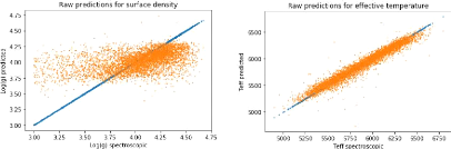
(a) Predictions for surface gravity: huge bias. (b) Predictions for effective temperature: well fitted.

Figure 11: Predictions of surface gravity and effective temperature for a multi-tasking three linear layers net with sizes 7 x 1024, 1024 x 512 and 512 x 3, trained for 20 epochs and with a learning rate of 0.001 using the one cycle policy.

Figures 11 and 12 show the results we get for a three linear layers net with sizes 7x1024, 1024x512 and 512x3. The effective temperature predictions seem quite smooth (Fig. 11b) but for the surface gravity we can see a huge bias on Figure 11a. This means that the net is working nicely on Teff like it does for the metallicity but for surface gravity it may be too simple. Multi-tasking is not really helping to guess better metallicity for a net that simple. In fact on Figure 12a, the predictions don't seem to be better than without multi-tasking, and we get a precision of ó 0.216dex.

(a) Scatter of the error on the predictions with regard (b) Histogram and fitted Gaussian for the difference between predictions

Figure 12: Results and precision for a multi-tasking three linear layers net with sizes 7x1024, 1024x512 and 512 x 3, trained for 20 epochs and with a learning rate of 0.001 using the one cycle policy.

fast.ai has only few options for tabular data, so to get better results, we turned to a new algorithm that uses directly the PyTorch module. This has been accomplished with the assistance of Foivos Diakogiannis, an AI researcher at the University of Western Australia (Perth). We also use new spectrometric data from LAMOST (Large Sky Area Multi-Object Fibre Spectroscopic Telescope), which provides a wider number of stars. We also play with all the colors in inputs, meaning the g,r,i,z bands are doubled: one of each is coming from Pan-STARRS and another from SDSS. This leads us to a total of 12 colors as inputs, which we can choose to use or not by turning Booleans to True or False.

We first need to wrap up data properly to get it ready to be trained on. To do so, we create a get_data_as_pandas() function which reads our fits file and converts it to pandas, with possibility to shuffle data. Working with joined surveys, we have a lot of unwanted fields so this function keeps only the one we need as inputs or outputs, i.e. multi-band photometry, spectrometric output as required (depending on if we want to do multi-tasking) and associated uncertainties. In fact, uncertainties allow to do data augmentation if needed and can be used in a customized loss function to prevent the net from learning too much from not well measured stars.

Then we need a new data set class to wrap up, define training and validation sets and normalize all of it. We call this new class AstroDataset and implement its methods. The first one is the initialisation: we use our get_data_as_pandas() function to get a raw data frame, which is then normalised. The normalisation is done separately for the training and the test sets, in order to not influence the training with values used on the test set and getting a test set truly unseen during training, and all means and standard deviations are stored for they will be needed for denormalisation afterwards. This first method also allows to define in which mode to consider the AstroDataset: train mode for training, test mode for validation or all to get the whole data set, useful for example when we want to get predictions for a whole data set once the net is trained enough. The two other methods are len and getitem functions, which are basics in data sets. They respectively allow to obtain the length of the data set in question and access to one or several of its element(s). The getitem method separates the inputs from the outputs when it is called. For our needs, it separates it in five categories: the inputs (photometry), spectroscopy, measurement errors on spectroscopy, 'pop' parameter (see in Section 4.4) and errors on 'pop' parameter.

The architecture of our new net is inspired from the ResUNet-a framework developed by Diakogiannis et al. 2020 [5] in order to deal with scene understanding of high resolution aerial images. It uses UNet encoder/decoder backbone combined with residual connections, multi-tasking inference and other complicated machine learning techniques.

The encoder/decoder architecture allows to go deeper and deeper into inputs to find features at different scales. It is easy to understand regarding translation. For example to translate the sentence THE DARK SIDE OF THE FORCE from English to French, the net first feeds on it and encodes each word into a number: the inputs become what is called a context vector containing numerical codes for the words to be translated. Then this vector is fed to a decoder and translates the numbers into French: LE CÔTÉ OBSCUR DE LA FORCE. Literally, the translator would guess LE OBSCUR CÔTÉ, since French and English people do not agree on the order of words in sentences. In fact, a simple net feeds on the inputs and forget them afterwards, soit would probably give this kind of error, even if an encoder/de-coder architecture would naturally inspect the sentence at various scales. To compensate, residuals are used at each step of the architecture so that information contained on inputs can persist. Those techniques apply perfectly on images: to go deeper in an image means to look for smaller and smaller features, and the persistence of information allows to analyse those features keeping on mind the context. Ronnenberg et al. 2015 [7] created the U-Net architecture for biomedical image segmentation, net that inspired Diakogiannis on his work and so on ours.

Another interesting technique is attention. Attention in machine learning is used to rank input data in order of importance. It is a computing translation of how we humans pay attention to important details linked to one another in an image, a sentence or a table, and how the background (i.e. less important pieces of information) seems blurred. For example in computer vision, to recognize a dog's face it is essential to identify its nose, eyes and ears and to compare their positions, sizes or colors, but the details of the background are not important. Recurrent neural networks already allow information persistence, but attention brings an order to it. It can be seen as an importance weights vector, which quantifies the correlation of a datum to other data.

This new architecture proposed by Diakogiannis et al. 2020 [5] can be adapted to work with 1D data such as ours. To implement it, we create a residual building block class called ResDense_block, and from those blocks we create a net class called AstroRegressor . They both have two methods: init for initialisation where the layers to be used are declared and forward for implementing the computational graph, i.e. the way the layers are linked to one another.

Building blocks are handy when it comes to repetitive networks. For example on fast.ai, the get_tabular_learner function uses linear building blocks, as can be seen on Figure 4 with the repetition of Linear-ReLU-BatchNorm-Dropout layers. The ResDense block we implement is quite similar to those. In fact, it is a simple net with only one activation funtion (ReLU) and 4 declared layers: one BatchNorm layer BN1, one linear layer dense1, another BatchNorm layer BN2 and another linear layer dense2. The difference comes in the forward method, where we implement the computational graph as shown in Equation 4.3.1: the output out is computed by feeding the inputs in to the simple net and adding it back at the end as residuals.

The AstroRegressor class is then created using the ResDense blocks. Its init method is quite heavy since it has to define both the encoder, the decoder and the last layers to define the outputs, which we call heads and are detailed in the next subsection. The en-coder/decoder backbone must absolutely symmetric. It can be defined using the minimum and maximum numbers of features only, meaning the minimum and maximum sizes of the inner linear layers, and then it is scaled with power of 2. For example for (nfea-tures_init, nfeatures_max) = (64, 2048), the encoder and decoder sizes would be as follows:

Encoder: 64 x 128 -+ 128 x 256 -+ 256 x 512 -+ 512 x 1024 -+ 1024 x 2048 Decoder: 2048x1024-+1024x512-+512x256-+256x128-+128x64

This is often done because of the belief that computer science works better with powers of 2. The problem is, to get a deep net using this strategy brings to a huge amount of parameters. To keep it lighter, we define our AstroRegressor by giving it still nfeatures_init and nfeatures_max but also an effective depth, which quantifies the depth at which the middle layer is reached. It requires an additional function to get the features scale, which we define as another class called features_scale. Figure 13 shows an encoder/decoder backbone obtained using this class with (nfeatures_init, nfeatures_max) = (64, 2048) and depth = 12. This net is deeper and less heavy than a net with features scaled by a power of 2 for a depth of 12, which would go to 2¹⁷ for nfeatures_max.

Figure 13: An example of encoder/decoder architecture built using ResDense blocks and AstroRegressor class working with depth. Are given effective depth of 12 and minimum and maximum numbers of initial features of 64 and 2048 respectively. The going up part (left) is the encoder and the going down part (right) is the decoder.

We also create a residual building block with attention class called AResNet block net with attention class called AttAstroRegressor. The AttAstroRegressor architecture is not really different from the AstroRegressor one, the main changes are in the building blocks. The AResNet block is itself based on the ResNet block with added an AttentionDense layer.

The last block is the one that defines the output(s), referred to as head. It is also called classifier because it dispatches the outputs, but as can be understood later, this name would be unsettling. It is this layer that defines if we just guess metallicity, or try multi-tasking, or else. For a simple guess of metallicity or for "simple" multi-tasking, we can use a simple head, which is essentially a linear block. This is what our first fast.ai

net did and what is shown in Figure 14a: out_features can be 1 if we want to guess only metallicity but also can be 2 or 3 if we want to add effective temperature and/or surface gravity and do multi-tasking.

A new idea is to create a classification output to help the net converge. In fact, we get predictions for the whole dataset using a previous satisfying version of the net, one with precision of ó 0.15dex, and create a new field called pop in which we put 1 when the prediction is bad ans 0 when it is good. With the same inner architecture but a special head and a special loss function (see in next Subsection), we can turn the regressor into a classifier. And by defining two different heads, one for regression and one for classfication, it is possible to do both at the same time. For consistency, an uncertainty field must be added in the AstroDataset class so we create artificially an epop column which is all ones when the dataset is deployed for training and all zeros when for validation.

Machine learning is the art of recognizing links between inputs and outputs, so to improve the net we can add causality in it. Causality means to add order in the predictions. For example and as illustrated on Figure 14b, we can have one head on the last layer of the backbone to first guess effective temperature, then use this guess with the backbone to guess surface gravity with a second head and finally use _Teff, log(g) and the backbone to guess metallicity. This can help creating links but this can also transpose bias from one output to another. In fact, as we saw in the previous Section, log(g) predictions are strongly biased so it may contaminate metallicity predictions, thus the importance of the order.

Figure 14: Definition of head(s) whithin AstroRegressor class init method. (a): one head for regression only, out_features defines the number of outputs and each are computed independently. The outputs are obtained by applying the regressor directly after the decoder. (b): several heads for causality with regressor and classifier, conv_dn is the table coming out of the encoder/decoder backbone. _Teffis first computed from conv_dn , then [Fe/H] from (conv_dn,T_eff ), then log(g) from (conv_dn, Tef f , [Fe/H]), then classification from (conv_dn, _Teff, [Fe/H], log(g)). Outputs are Teff, FeH and logg concatenated, and giant_pred.

Many things occur during training, so we create various functions to optimize the training loop. First, the loss function must be adapted to the heads. For regression, we create a customized loss function called custom_loss, working with predictions, expectations and uncertainties. It gets the difference between expectations and predictions in absolute value and divides it by normalised uncertainties: it is a weighted loss, which aims to make the net learn more from stars with low uncertainties than with high ones. Then it returns a mean of the loss over the dataset it is fed on. For classification, we choose to use BCEWithLogitsLoss(), which is Binary Cross Entropy with one Sigmoid layer. For both regression and classification, we use respectively our custom_loss and BCEWithLogitsLoss() and use the sum as a total loss. To make sure one doesn't take advantage on the other, we add a parameter á to the sum and weight each sub-loss with respectively á and 1-á. We adjust the á parameter accordingly to the convergence speed during training. Be it for regression, classification or both, the training loss is computed directly inside the training loop.

For the validation loss, we create a function to evaluate it to be used in the training loop, called eval_test_loss. This function uses the same loss function than in the training loop but applies it to the validation set and gets a mean of the loss over all the validation set. The aim is to train the net and go for the lower validation loss, so using the result of this function in the training loop, it is possible to save the parameters of the net each time it improves and by doing so, always have the best fit model to check out its precision, and not the last updated version as it was the case using fast.ai. This is called checkpoint-ing. Also, having both training and validation losses stored in a 'history' list, it is possible to plot the progress of the net at each epoch. To do so, we create the generate_image function which plots the evolution of training and validation losses as a function of the epoch, with adaptive edges, as shown in Figure 16a. The red dot corresponds to the best validation loss for which checkpointing saved the model.

Before entering the training loop, we must load the data we want to work on using the AstroDataset class and the DataLoader from torch module which allows to organize data onto batches and shuffle it if needed (needed for the training session but not the test session). Then we must define our net using one of the AstroRegressors (with or without attention) we created and choose an optimizer. We keep the Adam optimizer which is the default set for most nets and works well in many cases. We then must define our first learning rate and number of epochs we want the training loop to run for, which are both to be adapted accordingly to the net's response, i.e. the evolution of the losses. The learning rate is passed as an argument to the optimizer so to be able to change it inside the training loop, we create a function which puts the optimizer's "lr" parameter to the new value. A last value to set is the initial value for checkpointing: we fix acc=1.0e30 to be sure this threshold is passed on the first epoch.

Now the training loop can begin. At each epoch, we first put the net in train mode and set the initialise the training loss to 0. Then for each batch on the training set, we reinitialise the optimizer gradients to 0, we get the inputs, the expected outputs and their uncertainties and we send it to the GPU. Once we have the inputs we can do the forward pass by feeding them to the net and get the predictions, and from those and the expected

output we can compute the loss using our favourite loss function. Now it is time for the backward pass: we compute the gradients using the loss.backward() command and update our net's parameters using the optimizer.grad() command. Then the value of the loss for this batch is added to the training loss. At the end of the batch loop, the validation loss is computed using the eval_test_loss function and and both training and validation losses are added to the history list, in order to be plotted at the end of the epoch using the generate_image function. The last action of the training loop is to check if the net get better, i.e. if the validation loss get lower on this epoch, and if it did, it saves the parameters of the net under a chosen name.

This training loop is destined to trial and error. In fact, there is no one cycle policy here so the learning rate has to be changed manually when the net doesn't get more precise anymore or when it doesn't learn enough. The aim is to train it again and again until the validation loss starts to diverge to ensure that the best value is truly reached, and it can take a few hours.

To get our results, we create a get_preds function which basically puts the net in test mode, feeds it the validation set and gets the predictions. It returns the predictions and the expectations so we can compare both. We can then plot the scattering of our results for regressions as did with the fast.ai net and as shown on Figure 15. To visualise the results of the classification part, we create a function to plot its confusion matrix. This matrix shows on the x-axis the predicted labels and on the y-axis the true labels, then a color code shows the number of objects well and wrongly predicted. That is what shows the top left panel on Figure 15.

We can see on Figure 15 that biases for metallicity and effective temperature are still quite low compared to our results with the fast.ai net, but the surface gravity plot evolved remarkably. The bias is way lower than with the old net (see Fig. 11a for comparison), showing that our improvements were efficient. The top left and bottom right cells in the confusion matrix correspond to the well identified stars. They are way darker than the two other cells, meaning that our classifier is working nicely. Those first visual results are satisfying.

Finally, Figure 16b shows the precision we obtain for an encoder/decoder backbone net using attention and multi-tasking on metallicity and surface gravity, with a depth of 6, a minimum number of features of 32 and a maximum of 4096. With this net, we get a precision of ó 0.1446dex, which breaks the 0.2dex record of Ibata et al. [4] the 0.15dex one of Thomas et al. [3].

Figure 15: Visualisation of the predictions given by a regressor and classifier multi-tasking net with attention, with the backbone shown in Fig. 13 (nfeatures_init=64, nfeatures_max=2048, depth=12). Top left: confusion matrix for the 'pop' parameter. Top right, bottom left, bottom right: scattering of predicted effective temperature, surface gravity and metallicity respectively.

Figure 16: Training and results for a regressor only [Fe/H] and log(g) guessing net with attention and with an encoder/decoder backbone of depth = 6 and nfeatures_max = 4096. (a): History of the last epochs of training, in red the best validation loss for which the model was saved. (b): Histogram of the difference between predictions and expectations and fitted Gaussian, with values of amplitude, mean and standard deviation at the top respectively from left to right. Precision of the net: ó 0.1446dex.

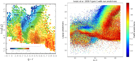
We use this last net with precision of ó 0.14dex on a huge photometric catalog containing data from Gaia, PS1, SDSS and CFIS, to get photometric estimates of metallic-ity and surface gravity, i.e. measures of those two spectrometric parameters, but based on photometry. This gives us the photometric estimates of 18,183,767 stars. Let's then compare it to the estimates of Iveziéet al. 2008 [2].

We propose to compare our metallicity and surface density estimates to Iveziéet al. [2] work, using their Figure 1, which displays mean metallicity color scale as a function of (g - r) color and surface gravity. This figure is visible on Figure 17 left panel. In particular, it allows us to identify giant stars in the log(g) < 3 region, which represents 4% of the objects in this plot. This region is dominated by low metallicity stars with [Fe/H] < -1. Two types of giants are visible on this figure: Blue Horizontal Branch (BHB) stars and red giants.

We do the same color cuts and plot raw metallicity. That is what is plotted in the right panel of Figure17. The fraction of giants in this plot is 2% so we found fewer giants than Ivezié. The rainbow feature corresponding to the red giants is easily identifiable on our plot, but the much rarer BHB stars are under-represented.

Figure 17: Comparison of metallicity as a function of (g - r) color and surface gravity between Ivezié's Figure 1 (left) and the same plot with our results (right). Color cuts are g<19.5 and -0.1<g-r<0.9. On the left panel, the dashed lines correspond to main sequence (MS) region selected for deriving photometric estimates for effective temperature and metallicity. The giant stars (log(g)<3) can be found for -0.1<g-r<0.2 (Bue Horizontal Branch stars) and for 0.4<g-r<0.65 (red giants). The features corresponding to red giants are easily identifiable on our plot in the right panel, but not the BHB stars. However, a strong low metallicity line appears for 0.4<log(g)<0.45.

Spectroscopic parallaxes are computed using magnitudes. In fact, Equation 5.2.1 shows the way to get heliocentric distances dist using absolute magnitudes M_rand apparent magnitudes m. The m - M_rterm is referred to as the distance modulus and noted u.

m-M_r= 5log10

u di st 10pc

? dist= 101+u/5 (5.2.1)

The apparent magnitude of an object comes from photometry and Ivezic et al. 2008 [2] developed a process to get its absolute magnitude from its metallicity. As shown by Equation 5.2.2, absolute magnitude can be decomposed on two factors: one depending on (g - i) color called M0 r and one depending on metallicity called AM_r.

Iveziélooked for a relationship between those values, fitting it for five known globular clusters. Observations led to look for two polynomial fits, one linking (g - i) color to M0 r and one linking metallicity to AM_r. They came up to Equations 5.2.3 and 5.2.4 below.

We apply this process to compute heliocentric distances, and then transform to Galactic cylindrical coordinates. We have at our disposition right ascension and declination from Gaia, so we use topcat to convert these to Galactic longitudes and latitudes, later noted respectively l and b. To convert those into cylindrical coordinates, we use the trigonometrical relationships shown in Equations 5.2.5 and 5.2.6. The values of cylindrical radius and distance to the galactic plane for the Sun come from two different studies: R= 8.122#177;0.031kpc from Abuter et al. 2018 [8] and Z= 0.017kpc from Karim et al. 2016 [9].

To compare our results with Ivezié's work, we reproduce Figure 8 from his article, showing the dependence of the median photometric metallicity as a function of the cylindrical radius R and the norm of the distance to the Galactic plane |Z| for data from SDSS DR6. This figure is our Figure 18 hereafter. The choice of coordinates puts the Galactic center at the (0,0) point and the Sun at about (8,0.1). An interesting feature to notice is the metallicity gradient which is quite linear with |Z|. The halo is made of stars with low metallicities and the closer to the disk one gets, the higher the metallicities. This change in metallicity allows us to identify the halo (dark blue) and the thick and thin disks (green to red) of the Milky Way, but also the Monoceros stream as pointed out on the figure.

We apply the same color, distance and metallicity cuts to zoom on the same region, our sample being put down to 1,180,853 stars. We choose to first reproduce Ivezié's map

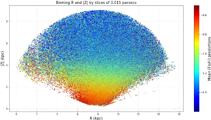
Figure 18: Iveziéet al. Figure 8: Dependence of the median photometric metallicity for about 2.5 million stars from SDSS DR6 with 14,5<r<20, 0,2<g-r<0,4, and photometric distance in the 0.8-9 kpc range, in cylindrical Galactic coordinates R and |Z|. There are about 40,000 pixels (50 pc ×50 pc) contained in this map, with a minimum of 5 stars per pixel and a median of 33 stars. Note that the gradient of the median metallicity is essentially parallel to the |Z|-axis, except in the Monoceros stream region, as marked.

using raw metallicity. That is what is shown in Figure 19: |Z| as a function of R with raw metallicity as color scale. We find back that the stars of the disk have higher metallici-ties than the ones in the halo, but the smooth metallicity gradient showing the difference between thin and thick disks and the Monoceros stream disappeared. For the latter, the difference of footprint is probably responsible, since our sample does not contain all the SDSS data.

To uncover the smooth gradient, we compute and display mean metallicities instead of raw ones. To do so, we bin the data on R and |Z| in slices of 0.015 parsecs and get a mean for the other parameters. 0.015 parsecs is a good compromise between clarity of results and number of data remaining. In fact in Figure 20, the wings of the plots are a bit weak but information remains: the smooth gradient appears.

Figure 19: Dependence of raw predicted metallicity for about 1.18 million stars from Gaia, PS1, SDSS and CFIS joined together with are 14.5 < r < 20, 0.2 < (g -r) < 0.4, 0.8kpc<dist<9kpc and -1.6<[Fe/H]<-0.5, using Galactic cylindrical coordinates R and |Z|. Due to difference in metallicity, the disk appears reddish on the bottom of the plot and the halo is mainly blue, visible for |Z|>4kpc.

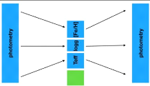
Figure 20: Dependence of mean predicted metallicity for about 1.18 million stars from Gaia, PS1, SDSS and CFIS joined together with are 14.5 < r < 20, 0.2 < (g -r) < 0.4, 0.8kpc<dist<9kpc and -1.6<[Fe/H]<-0.5, using Galactic cylindrical coordinates R and |Z|. Binning is of size 0.015pc x 0.015pc in R and |Z|. The disk and halo are still visible in the same colors but now the smooth gradient appears.

One limit of the network we developed so far is that it requires a certain amount of fields in the dataset, exactly seven colours, which keeps stars with less photometric information getting a prediction of their metallicities. We thus want to create a similar net which predicts the same spectrometric parameters but with one colour missing. To that end, we create an auto-encoder. Its aim is to extend the previously developed net to datasets with one colour missing and also get a prediction for this colour. This allows to increase the number of stars for which our net can estimate the metallicity.

Figure 21 shows the principle of the auto-encoder, which has two steps. The first step called encoder is a net identical to the previous one but with one colour missing, soit predicts the spectrometric parameters we want. The second step called decoder is mirror net which takes the spectrometric parameters as inputs and predicts the missing colour. To manipulate the missing colour, we create an index called missing_band. It is to be used identify the missing colour field inside the dataset during training. For easier understanding, the encoder/decoder architecture we described in Section 5 is from now on referred to as a sandwich net.

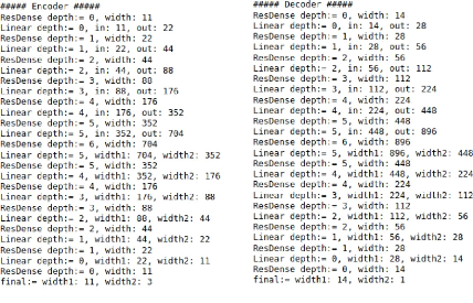
Figure 21: Scheme for an auto-encoder: left arrows represent the encoder, right arrows are the decoder. The green square is a hypothetical parameter to be added if it doesn't work with Teff, logg and FeH only.

The architecture of the auto-encoder is thus composed by two sandwich nets, as shown in Figure 22, each one's role being defined by their first and last layers. The encoder aims to predict the effective temperature, the surface gravity and the metallicity from the 11 colours we have as photometric inputs minus the missing band, that's why the first layer is of size 11 and the last one is of size 3. The decoder aims to predict the missing band starting from all the photometric and spectrometric data we have, so its first layer is of size 14 and its last is of size 1. The layers within the sandwich nets are ResDense building blocks of a given size or linear layers to increase or decrease linearly the size of the following ResDense layer.

In practice, we define subclasses to help implement the auto-encoder. We first implement the sandwich net class, which is the previous 'encoder/decoder' structure we implemented in Section 4. It takes the input and output sizes as explained in the previous paragraph, and create a sandwich structure of ResDense and linear layers corresponding

Figure 22: Structure and inside sizes of the auto-encoder. (a): the encoder composed of a sandwich net of depth 6 and predicting Teff, logg and FeH (width2=3 in the final layer). (b): the decoder composed of a sandwich net of depth 6 and predicting the missing colour (width2=1 in the final layer).

to each part of Figure 22. Then we create an Encoder class and a Decoder class to implement separately the encoder and the decoder with the right input and output sizes. Finally, we create an AutoEncoder class to implement the final common structure, and organize the forward pass. We fix in this method the part of the input data on which the net feeds.

The main difficulty we encounter doing those modifications is the consistency between the sizes of the nets and the data going through it. This consistency is to be reached to make sure the data on which the nets are feeding are the good ones, so photometry minus one colours for the first and spectrometry plus photometry minus one colour for the second. Basically, it all depends on the definition of the getitem method inside the AstroDataset class and how it is used in the eval_test_loss and get_preds functions and inside the training loop. We decide that the getitem function has to separate the data whithin five categories: the inputs (photometry minus one colour depending on the index of the missing colour), ground truth spectrometry, errors on spectromectry, ground truth of the missing colour and errors on the missing colour. Those different categories are used in the forward pass to make sure that the first sandwich net feeds on the photometry minus one colour (the inputs) and the second feeds on the same inputs concatenated to the predictions of the spectrometric parameters. The ground truths and errors are used inside the custom loss function as before, in order to compute the training and validation losses.

We then modify the eval_test_loss() function, the get_preds() function and the training loop accordingly. To evaluate the loss between the ground truth and the predictions of the encoder, we use our custom_loss() function with special weights to give more or less importance to the parameters we want to predict. The most important being metallicity, we give it an artificial weight of 10, then 3 for surface gravity and 1 for effective temperature. Then for the decoder we just compute the mean of the absolute value of the difference between the ground truth and the predictions of the missing colour. The total loss is thus the sum of each sandwich net's losses. The rest of the eval_test_loss() function and the training loop are the same as before: we get the predictions, compute the losses and adjust the net through a backward pass. The training and validation losses are stored to plot the learning history during training. We also kept checkpointing, which allows to save the parameters of the net for the best value of validation validation loss.

We first try and train an auto-encoder with the (G - u) colour missing. As usual, we plot the evolution of the training and validation losses during training to see its evolution, as can be seen on Figure 23: the curves are quite bumpy but some converging parts appear, meaning the auto-encoder still learns.

Figure 23: Evolution of the training (blue) and validation (orange) losses as a function of the epochs. The red dot marks the lowest validation loss, for which the parameters of the net are saved. Between 0 and 200 epochs, the curves are very bumpy but then they converge.

To get a closer look to the results, we plot the predictions of the net after a few hundreds epochs in Figure 24. The spectrometric parameters don't seem too problematic but the missing colour is far away from satisfactory. To get a more accurate measure of the precision of the net, we can compute the differences between the expectations and the predictions for both metallicity and missing colour, histogram them and get their standard deviation ó, as shown in Figure 25. With more training and an adaptive learning rate, we could probably a better precision for both parts. We could also add an artificial weight in the loss for the missing colour like the ones added in the loss for the spectroscopic parameters. Adding a weight of 10 for example would balance the loss and increase the impact of the missing band on the adjustment of the net during the backward pass.

Figure 24: Predictions of (g-r) colour in top left, effective temperature in top right, surface gravity in bottom left and metallicity in bottom right for a learning rate of 10^-3and a hundred epochs.

Figure 25: Precisions, histograms and fitted gaussians for metallicity (left) and (g-r) missing colour (right).

One challenge of Astrophysics is to estimate heliocentric distances, and techniques to measure them are called parallaxes. Geometric parallax is an efficient method but looses in precision with distance. However, Iveziéet al. 2008 [2] developed a way to compute spectroscopic parallax based on absolute magnitude recovered from metallic-ity. Moreover, with multi-band photometry, it is possible to cover whole spectra of million of stars at one go and get a huge amount of data quicker than with spectroscopy, which easily leads to big data and machine learning.

The aim of this internship was to create a neural network to propagate spectroscopic parallaxes to all stars with known multi-band photometry. This net had to learn to associate photometric data (magnitudes in u,g,r,i,z bands from Pan-STARRS, SDSS and CFIS and G,Bp,Rp bands from Gaia) to spectrometric data (metallicity, surface gravity and effective temperature from SEGUE) in order to predict it for stars with no spectrometric data available.

We ended up with two nets. The first one created with a simplified programming language called fast.ai, allowed to enter the world of machine learning in a top down point of view and getting acquainted with the main notions of this domain. The second one created using the Python module PyTorch, and with the fabulous assistance of Foivos Diakogiannis, was brought to work in a bottom up consideration, coding classes and functions used for our first net and more from scratch. This second net was the most efficient, reaching a precision of ó 0.1446dex.

This net was then used to estimate metallicities of about 18 million stars, which were used to compute their heliocentric distances as proposed by Iveziéet al. 2008 [2]. Those distances were used to plot a map of the distribution of metallicity inside the Milky Way, on which the halo, thin and thick disks were clearly identifiable.

We finally developed an auto-encoder, which aim was to extend our previous net to less complete entry datasets and to provide predictions for this missing colour(s) in addition to the spectrometric predictions. For a dataset missing the (G - u) colour, we get a precision of ó 0.169dex for the metallicity and ó 0.2 for the missing color.

With more time we could improve this auto-encoder to get a really satisfying precision. To prove its efficiency, we could train it on the (g - r) colour and get predictions for this colour, surface gravity and metallicity and then use them to reproduce our Figure 17, for which we would have the results of Iveziéet al. 2008 [2] and our first net as a comparison. It would also be interesting to test other bands and see the dependence of the precision as a function of it. Finally with significantly more time, we could try to find the optimal amount of photometric information to get satisfactory precision.

This internship allowed me to acquire a solid knowledge basis of Machine learning and its implementation using Python, which is a domain I find highly interesting and promising for the years to come. Furthermore, the discovery of fast.ai and learning it by myself during the first month made me work on my autonomy when handling a part of a project, and then learning to use PyTorch with both Rodrigo and Foivos was a great moment of team work. I am glad this project helped me develop both competences.

The conditions of this internship were especially demanding because of the Covid-19 pandemic. I am thankful that I was allowed to continue it and not forced to stop after only one month like happened to some other TPS interns in Strasbourg, but it was challenging. The lock-down was emotionally rough, particularly in Alsace which was the main cluster in France, and settling in teleworking outside the master room without having a dedicated room for work was quite hard at the beginning. Nevertheless, after a few complicated days, it allowed me to better organize myself in my work and to adapt to extreme conditions. Regular and warm communication with Rodrigo (and Foivos) via e-mails or Slack helped a lot.

This experience was an interesting leap into the research world. They allowed me to get a further glimpse to it and to understand how it works within Rodrigo's project. Using this insight, I could decide with more confidence what I want for my professional career. Astrophysics are a part of science that I love, and to be able to understand the discoveries that are to come in this domain. It taught me to be curious about the Universe in which I live while staying humble considering what I really understand of it. Even though I am not carrying on with a thesis, I am going to apply this scientific principle to my future job and life and stay in touch with Astrophysics.

In conclusion, those 6 months of internship were both a challenge and a pleasure. They shaped my future career and the person I am going to be in my professional life. I am deeply grateful to Rodrigo to have made all of this possible, for his eternal cheerfulness and warm encouragements. This experience prepared me to enter the labour force with more serenity.

[9] M. T. Karim and Eric E. Mamajek. Revised geometric estimates of the north galactic pole and the sun's height above the galactic mid-plane. Monthly Notices of the Royal Astronomical Society, 465(1):472-481, Oct 2016.

Machine learning for big data in galactic archaeology

3.4 First estimates of metallicity

3.5 Multi-tasking