2.4. Results
? Estimation of the realised niche from uncorrected
and corrected reference matrices
Data occurrences from the uncorrected training sets were first
used to determine the realised niche of each fish (Fig. III.S10). The contours
of these niches depended on species. Some species exhibited a unimodal
distribution close to a normal distribution. For example, the examination of
the thermal tolerance of haddock (Fig. III.S10(f)) showed a preferendum ranging
between 5°C and 15°C and an optimum around 9.75°C. Pollack was
more stenotherm, found between 9°C and 15°C with a thermal optimum at
about 12.75°C (Fig. III.S10(d)). However, for other species and
parameters, the distribution could be multimodal (e.g. Atlantic horse mackerel
and European anchovy; see Fig. III.S10(a), (b)). For all species, the
bathymetric distribution did not follow a normal distribution. The frequencies
of occurrence were maximal for the first 200 meters (i.e. continental shelf).
The contours of the niche for annual SSS were not as well defined as for the
other parameters because the amplitude of variation in the region was not
generally important. All species showed mainly a maximum of occurrence between
30 and 40. Pollack was less euryhaline than species such as common sole and
turbot (Fig. III.S10(e), (h)). The different salinity profiles exhibited by the
species highlighted the importance of the parameter as a predicting variable in
NPPEN.
Multiple modes are less conform to our common idea of the
ecological niche. They can be related to the absence of a specific habitat or
to the presence of oversampled or undersampled regions. They could also be due
to seasonal migration such as the one performed by sardine. Indeed most often,
data used in ENMs do not originate from rigorous sampling protocol (Legendre
& Legendre 1983). To consider this bias, the training set was corrected,
which resulted in an improvement of most environmental preferendums (Fig.
III.2). However, the procedure of correction did not modify substantially the
environmental profiles of species, indicating that the profiles were here not
too much influenced by the heterogeneity of the spatial information. Most
optimums were refound (Fig. III.2). In the case of poorer occurrence dataset
(e.g. turbot; Figs. III.S10(h) and 2(h)), the correction allowed contours of
the salinity preferendum to be completed. This homogenisation procedure enabled
some response curves to be better balanced. Such a correction was essential as
most ENMs, as ours, are highly sensitive to the determination of the niche
? Sensitivity of the model to bimodality and sampling
density
Previous results showed that some species exhibited multimodal
responses (Figs. III.S10 and 2). To evaluate the influence of such
patterns on our model, we simulated training sets characterised by different
types of bimodality and sampling density (Fig. III.3). This comparisonwas made
by simulating the values of two environmental parameters: SST and bathymetry.
When the density of sampling was regular and in case of unimodality, the
highest probabilities were observed at the centre of the sampling points and
declined progressively towards the edge of the distribution (Fig. III.3(a)).
This training set was considered here as a reference to evaluate simulated
incomplete, heterogeneous and bimodal training sets. The model was robust to
incomplete or heterogeneous training sets (Fig. III.3). The mean difference
ranged from 0.0940 (Fig. III.3(b)), 0.0732 (Fig. III.3(c)) to 0.0622
(Fig. III.3(d)). These results suggest that the model was quite robust to
altered training set that could be related to incomplete sampling coverage or
an unrepresented biotope.
Figure III.4 : Estimated probability of
occurrence using the model NPPEN for the decade 1960-1969, the time period
2000-2005 in the North Atlantic Ocean. (a) Atlantic horse
mackerel, (b) European anchovy, (c) European
sprat, (d) pollack, (e) common sole,
(f) haddock, (g) saithe and
(h) turbot. The western boundary of the model was fixed to
40°W. This was arbitrary selected for species (but haddock and saithe),
which are only found on the eastern side of the Atlantic Ocean.
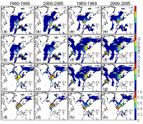
? Modelled spatial distribution of fish species
(contemporaneous spatial patterns)
The examination of the modelled spatial distribution for the 8
species considered in this study indicated the presence of three groups (Fig.
III.4, period 1960-1969): (1) species with a spatial distribution mainly
centred in the Celtic Sea and/or the North Sea (called temperate species;
European sprat, pollack and turbot); (2) species with a spatial distribution
from southerly regions to the North Sea (called warm-temperate species;
Atlantic horse mackerel, European anchovy and common sole); (3) species with a
spatial distribution ranging from the North Sea to the Barents Sea (called
subarctic species; haddock and saithe). These results showed that the North Sea
and more generally regions close to the British Isles represented a
biogeographical crossroad between the Atlantic Arctic and the Atlantic
Westerlies Wind (temperate) biomes (Longhurst 1998). The probability of fish
occurrence calculated from NPPEN exhibited substantial differences with the
maps produced by the FAO (Fig. III.S1).
? Comparison of the spatial distribution inferred from
NPPEN and AquaMap
We compared the spatial distribution of fish occurrence
modelled by NPPEN for the 1960s and the period 2000-2005 with outputs from
AquaMap (Kaschner et al. 2006) by correlation analysis (Table III.1).
The strength of the correlations, similar for the two periods (190-1969, mean
correlation: 0.5075; 2000-2005, mean correlation: 0.53), depended on species.
Although all coefficients of correlation were significant, the amount of
variance explained ranged from 1.44% for European anchovy to 56.25% for haddock
(Table III.1). The minimum degree of freedom needed to have a significant
correlation was calculated to evaluate in which measure the spatial
autocorrelation could have influenced the results. For example, the high
correlation found with haddock remained significant (p= 0.05) with only 5
degree of freedom (Table III.1). The reduction of the degree of freedom ranged
from 5 to 255 (European anchovy). In general, the correlation between the two
models tended to increase with the number of occurrence data in the reference
matrix (correlation calculated between the decimal logarithm of the number of
data after simplification of the training set in Supplementary Table III.1 and
correlation coefficients in Table III.1; 1960-1969: rp=0.53, p=0.17;
2000-2005: rp=0.45, p=0.27).
Figure III.5 : Maps showing areas where
a substantial increase (in red) or decrease (in blue) in the probability of
occurrence (changes>0.2, see `Materials and methods') is expected between
the 2090s and the 1960s. Green areas denote no substantial change or changes
<0.2. (a) Atlantic horse mackerel, (b)
European anchovy, (c) European sprat, (d)
pollack, (e) common sole, (f) haddock,
(g) saithe and (h) turbot. The western
boundary of the model was fixed to 40°W. This was arbitrary selected for
species (but haddock and saithe), which are only found on the eastern side of
the Atlantic Ocean.
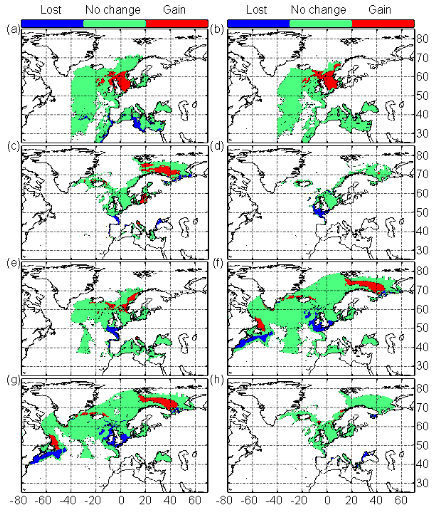
Table III.1 : Correlations between the
spatial patterns in the probability of fish occurrence between the model NPPEN
and AquaMap (Kaschner et al. 2006) for the period 1960-1969 and
2000-2005. n: degree of freedom; rp: Pearson linear coefficient of
correlation; p: probability; n.f.: minimum degree of freedom needed to have a
significant correlation at p=0.05.
|
|
NPPEN 1960/1969 - AquaMap
|
NPPEN 2000/2005 - AquaMap
|
|
Row
|
FAO species names
|
N
|
rp
|
p
|
n.f.
|
n
|
rp
|
p
|
n.f.
|
|
(a)
|
Atlantic Horse mackerel
|
63,021
|
0.49
|
<0.01
|
14
|
62,904
|
0.54
|
<0.01
|
11
|
|

(b)
|
European Anchovy
|
58,831
|
0.12
|
<0.01
|
255
|
58,722
|
0.14
|
<0.01
|
184
|
|
(c)
|
European Sprat
|
30,582
|
0.47
|
<0.01
|
15
|
30,503
|
0.47
|
<0.01
|
16
|
|
(d)
|
Pollack
|
19,865
|
0.71
|
<0.01
|
5
|
19,854
|
0.68
|
<0.01
|
6
|
|
(e)
|
Common Sole
|
41,029
|
0.52
|
<0.01
|
12
|
40,883
|
0.60
|
<0.01
|
8
|
|
(f)
|
Haddock
|
86,820
|
0.75
|
<0.01
|
5
|
86,286
|
0.72
|
<0.01
|
5
|
|
(g)
|
Saithe
|
76,009
|
0.61
|
<0.01
|
8
|
75,689
|
0.61
|
<0.01
|
8
|
|
(h)
|
Turbot
|
26,923
|
0.39
|
<0.01
|
23
|
26,796
|
0.48
|
<0.01
|

15
|
|
Row
|
FAO species names
|
Thermal preference
|
Period 2000/2005 ? 1960/1969
|
Period 2090/2090 ? 1960/1969
Scenario A2
|
Period 2090/2099 ? 1960/1969
Scenario B2
|
|
|
|
Gain
|
Lost
|
Balance
|
Gain
|
Lost
|
Balance
|
Gain
|
Lost
|
Balance
|
|
(a)
|
Atlantic horse mackerel
|
Warm temperate
|
173,865
|
56,125
|
117,740
|
956,524
|
969,816
|
?13,291
|
918,117
|
737,099
|
181,017
|
|
(b)
|
European anchovy
|
Warm temperate
|
375,539
|
29,205
|
346,334
|
1,020,267
|
39,302
|
980,965
|
984,187
|
17,768
|
966,419
|
|
(c)
|
European sprat
|
Temperate
|
285,696
|
83,857
|
201,839
|
601,395
|
419,186
|
182,209
|
598,114
|
328,168
|
269,946
|
|
(d)
|
Pollack
|
Temperate
|
36,505
|
47,779
|
?11,274
|
101,459
|
352,090
|
?250,631
|
56,010
|
315,461
|
?259,451
|
|
(e)
|
Common sole
|
Warm temperate
|
105,455
|
23,381
|
82,074
|
430,869
|
430,972
|
?102
|
435,829
|
321,902
|
113,926
|
|
(f)
|
Haddock
|
Sub-Arctic
|
341,083
|
266,414
|
74,668
|
899,733
|
1,311,603
|
?411,870
|
794,319
|
1,189,764
|
?395,445
|
|
(g)
|
Saithe
|
Sub-Arctic
|
281,311
|
278,110
|
3,200
|
908,634
|
1,503,825
|
?595,190
|
796,864
|

1,295,440
|
?498,576
|
|
(h)
|
Turbot
|
Temperate
|
59,873
|
101,639
|
?41,766
|
154,142
|
334,280
|
?180,138
|
147,409
|
216,425
|
?69,016
|

Table III.2 : Thermal preference and the
expected area (in km²) gained or lost by the species between the period
2000-2005 and 1960-1969 and 2090-2099 and 1960-1969 for both scenarios A2 and
B2. The balance was calculated (in km²) as the difference between gained
and lost area (see Materials and Methods).
? Observed changes in species distribution
All species but haddock exhibited a northward movement or an
increase in the probability of occurrence at the northern edge of their spatial
distribution between the 1960s and the period 2000-2005 (Fig. III.4). The
probability of occurrence of European sprat increased substantially in the
North Sea in 2000-2005. The reduction in the probability at the southern edge
of all species was not evident with the exception of European sprat, saithe and
haddock (e.g. the southern part of the North Sea). Between the 1960s and the
period 2000-2005, the potential habitat of warm-temperate species increased
(Table III.2). Among them, the potential habitat of European anchovy increased
substantially (balance of change: 346,334 km²). Both subarctic and
temperate species exhibit a weak or a moderate increase between the 1960s and
the period 2000-2005 or a moderate decrease for pollack and turbot (Table
III.2).
? Changes in species distribution
Modelled spatial distributions based on projected IPCC changes
in SST (scenario B2) suggest that northward movements in fish may accelerate in
the future with the exception of pollack in the North Sea (Fig. III.S10). These
movements will be generally associated with a reduction located at the southern
edge of the species spatial distribution (Fig. III.S10). The projections
suggest that the potential habitat of European anchovy will increase (Fig.
III.5, Table III.2). Results are less obvious for common sole or Atlantic horse
mackerel and suggested either a weak decrease (Scenario A2, Table III.2) or a
moderate increase (Scenario B2, Table III.2). Atlantic horse mackerel and
European anchovy are expected to move northwards along the European shelf-edge
and in the North Sea (Figs. III.S10 and III.5, Table III.2). The potential
habitat of temperate species is expected to decrease substantially
(Fig. III.5, Table III.2) with the exception of European sprat that is
expected to migrate to the Barents Sea. However, this species might eventually
disappear from the central part of the North Sea at the end of the century
(Fig. III.S10). The model suggests that the potential habitat of subarctic
species may diminish considerably (Fig. III.5, Table III.2). The reduction of
the potential habitat in the North Sea may not be overcome by the increase in
potential habitat over the Barents Sea. Projections based on scenario A2 and B2
for subarctic species gave very similar conclusions (Table III.2).
|
|


