Impact du réchauffement climatique sur la distribution spatiale des ressources halieutiques le long du littoral français: observations et scénarios( Télécharger le fichier original )par Sylvain Lenoir Université Lille 1 Science - Doctorat 2011 |

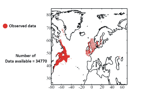
Annexe :Atlas climatique des ressources marines de l'Atlantique Nord Conjointement à cette étude, il a été réalisé un atlas des distributions spatiales et des changements attendus de ces distributions pour 51 espèces marines en Atlantique Nord, en utilisant le nouveau modèle NPPEN. Cet atlas est le fruit d'une collaboration avec SEAFISH industrie. Une présentation de l'atlas et un exemple des cartes de distribution y figurant ont été inclus en annexe, à la fin de ce chapitre. A climatic atlas of North Atlantic marine resources with a special emphasis on the English Channel and the North Sea Sylvain Lenoir, Grégory Beaugrand 1 Centre National de la Recherche Scientifique, Laboratoire d'Océanologie et de Géosciences' UMR LOG CNRS 8187, Station Marine, Université des Sciences et Technologies de Lille - Lille 1, BP 80, 62930 Wimereux, France E-mail: sylvain.lenoir@ed.univ-lille1.fr, Gregory.Beaugrand@univ-lille1.fr Report Contract for SEAFISH 31 Décembre 2008 How the two documents should be cited: Beaugrand G, Lenoir S (2008) A climatic atlas of North Atlantic marine resources with a special emphasis on the English Channel and the North Sea. Introduction and description of the procedures. Technical Report. Centre National de la Recherche Scientifique. Station Marine de Wimereux. Université des Sciences et Technologies de Lille 1. 17 pages. Lenoir S, Beaugrand G (2008) A climatic atlas of North Atlantic marine resources with a special emphasis on the English Channel and the North Sea. Technical Report. Centre National de la Recherche Scientifique. Station Marine de Wimereux. Université des Sciences et Technologies de Lille 1. 515 pages. A climatic atlas of North Atlantic marine resources with a special emphasis on the English Channel and the North Sea Introduction and description of the procedures Grégory Beaugrand, Sylvain Lenoir 1 Centre National de la Recherche Scientifique, Laboratoire d'Océanologie et de Géosciences' UMR LOG CNRS 8187, Station Marine, Université des Sciences et Technologies de Lille - Lille 1, BP 80, 62930 Wimereux, France E-mail: Gregory.Beaugrand@univ-lille1.fr, sylvain.lenoir@ed.univ-lille1.fr Report Contract for SEAFISH 31 Décembre 2008 How the two documents should be cited: Beaugrand G, Lenoir S (2008) A climatic atlas of North Atlantic marine resources with a special emphasis on the English Channel and the North Sea. Introduction and description of the procedures. Technical Report. Centre National de la Recherche Scientifique. Station Marine de Wimereux. Université des Sciences et Technologies de Lille 1. 17 pages. Lenoir S, Beaugrand G (2008) A climatic atlas of North Atlantic marine resources with a special emphasis on the English Channel and the North Sea. Technical Report. Centre National de la Recherche Scientifique. Station Marine de Wimereux. Université des Sciences et Technologies de Lille 1. 515 pages. The main objectives of this project were to model the spatial distribution of the main commercially exploited marine species in the North Atlantic sector with a special emphasis on the English Channel and the North Sea. Using a new type of model based on the use of the Generalised Mahalanobis distance and a Multiple Response Permutation Procedure, we propose scenarios of changes in the spatial distribution of 51 marine resources based on a climatic moderate scenario (Scenario B2; concentration of carbon dioxide of 621 ppmv by 2100). Results are presented as maps of probability of presence based on the decades 1960s, 2000s (observed and projected temperature), 2010s, 2020s, 2030s, 2040s, 2050s and 2090s (projected temperature). Overall, results show a migration of marine resources polewards at rate varying among species. It should be noted that some species will not have the possibility to move northwards as they might be restricted by other specific local or regional constraints related to the characteristics of the substrate (e.g. flatfish). A confidence index on projection is attached on each map for each species. It is based on the number of available data on which the ecological niche model is applied. Our project is attended to provide a first insight on the potential changes that could appear if climate continues to warm at a moderate rate. More sustained warming could trigger more rapid northward shifts. This atlas should be considered as a guideline against which changes in the resource might be better anticipated. Many uncertainties remain and the complexity of the system makes it difficult to consider these maps as exact predictions but rather as projections of potential distribution in the absence of biotic interactions which cannot be considered with our current level of knowledge. Materials and methods Fish data Data of cod occurrence was taken from Fishbase ( http://www.fishbase.org), ICES and other smaller datasets (Fig. 1). While high densities of data are present in the dataset on the western side of the North Atlantic, it is not so for the eastern side.
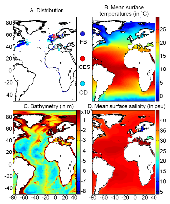
Figure 1 A. Spatial distribution in the data of presence of a fish reported found in the databases ICES, Fishbase or other smaller datasets (OD). B. Mean observed sea surface temperature for the period 1960-2005. C. Mean bathymetry in the Atlantic Ocean. D. Mean sea surface salinity in the Atlantic Ocean. Figure 1. Physical data Our projections are based on three abiotic parameters: bathymetry; salinity and sea surface temperature (use often as a proxy for conditions at the larval stage). Bathymetry data originated from a global ocean bathymetry map (1 degree longitude x 1 degree latitude)(Smith & Sandwell 1997). This dataset is among the most complete, high-resolution image of sea floor topography currently available. The map was constructed from data obtained from ships with detailed gravity anomaly information provided by the satellite GEOSAT and ERS-1(Smith & Sandwell 1997). Bathymetry data were considered because the spatial distribution of the Atlantic cod is in part explained by this parameter as the species occurs mainly over continental shelves (Louisy 2002) (Fig. 1). Annual Sea Surface Salinity (SSS, average values between 0 and 10 meters) data was obtained from the Levitus' climatology (Levitus 1982). ICES data were used to complete the Levitus dataset in coastal regions where there is no assessment of annual SSS (e.g. some regions of the eastern English Channel). ICES data were downloaded from http://www.ices.dk. Salinity was considered because it has a strong impact of the distribution of most fishes (Fig. 1). Sea Surface Temperature (SST) data originated from the database International Comprehensive Ocean-Atmosphere Data Set (ICOADS, longitudes with a spatial resolution of 1° longitude x 1° latitude; http://icoads.noaa.gov)(Woodruff et al. 1987). An annual mean was calculated for the period 1960-2005. Data on SST were considered as this parameter has strong impact on the spatial distribution of cod (Brander 2000, Intergovernmental Panel on Climate Change 2007) (Fig. 1). All physical data were bilinearly interpolated on a spatial grid of 0.1° longitude x 0.1° latitude at a global scale. While only one map of bathymetry and SSS (annual climatology) was generated, a grid for each year of the period 1960 to 2100 was built for SST (observed and projected). Therefore, spatial distribution in the probability of presence of a fish varies according to the three abiotic parameters while year-to-year changes are only function of SST. Mean values of bathymetry, sea surface temperature and salinity are presented for the North Atlantic in Fig. 2. Description of the Non-Parametric Probabilistic Ecological Niche model (NPPEN) The model is derived from a test recently applied to compare the ecological niches (sensu (Hutchinson 1957)) of two species (Beaugrand & Helaouët 2008). The analysis is based on Multiple Response Permutation Procedures (MRPP), a test first proposed by Mielke et al. (Mielke et al. 1981). MRPP has been applied in conjunction to Split Moving Window Boundary analysis to detect discontinuities in time series (Cornelius & Reynolds 1991). This method has also been utilised to identify abrupt ecosystem shifts (Beaugrand 2004, Beaugrand & Ibanez 2004). Mathematically, MRPP tests whether two groups of observations in a multivariate space are significantly separated. (Mielke et al. 1981 gave a full description of the test and Beaugrand & Helaouët {Beaugrand, 2008 #2205) have recently illustrated the procedure in details in an adaptation of the technique to compare two ecological niches.
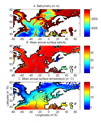
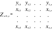
Figure 2 Spatial distribution of bathymetry (A), mean annual sea surface salinity (B) and mean annual sea surface temperature (C) in the North Atlantic Ocean. Isobaths 200m (dark grey line) and 2000m (light grey line) are indicated. The model we propose to assess the probability of occurrence of cod (and its changes in space and time) is in fact a simplification of MRPP. Instead of comparing two groups of observations, the analysis tests whether one observation belongs to a group of (reference) observations we call here the reference matrix. The reference matrix is represented by a matrix Xn,p with n the number of (reference) observations and p the number of variables. Each row of the matrix represents the environmental conditions where a species was detected. It is crucial that the reference matrix covers the entire niche (sensu Hutchinson) of a species to give reliable probability (Thuiller et al. 2004). This point, perhaps too often forgotten in this kind of exercise, was checked for each of the 51 species used in this paper. The predictive matrix Ym,p encompasses m observations of the environment using also p predictors. Each observation of Y, encompassing information on environmental conditions, will be tested against X (range of conditions where the species was detected). The model is applied in 4 main steps: Step 1: homogenization of the reference matrix In contrast to the terrestrial realm where the presence of a species can be more easily (visually) detected (at least for some species), this is not so for many species in the pelagic realm and especially for fish. The density of fish occurrence reported in the datasets depends on fishing activities. It is clear that the density of data points is higher in fishing area. Although this indicates to some extent that the resource is more abundant in those regions, this is not completely true. This phenomenon can potentially influence the outcome of any ecological niche model. Another phenomenon that can influence the probability is the wrong report of data occurrence. This can appear and it is not always possible to go through all individual observations. Misreports can profoundly influence the probability. In an attempt to overcome these drawbacks, we created a virtual cube (i.e. three controlling factors) with intervals of sea surface temperature of 1°C between -2°C and 18°C, intervals of bathymetry of 20m between 0 and 800m and intervals of salinity of 2 between 0 and 40 and retained one data occurrence when more than one observation were detected in the crossed intervals of SST, bathymetry and salinity. This threshold of two was fixed to eliminate the impact of one misreport. The resolution could, at first sight, appear to be coarse. However, the practice of the ecological niche model shows that the probability remains similar, even at low resolution (see Fig. 4). Step 2: preparation of data A matrix called Zn+1,p is created for each observation of Y to be tested against X. For the first observation, the following matrix is constructed:
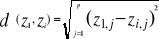
With xi,j, the observations in matrix X and yi,j, an observation of matrix Y. The building of matrix Z is repeated m times, corresponding to the m observations of Y. Step 3: calculation of the mean multivariate distance between the observation to be tested and the reference matrix MRPP was first proposed to be applied with an Euclidean distance, a squared Euclidean distance or a chord distance (Mielke et al. 1981). To first illustrate the technique, we use an Euclidean distance. Obviously, if variables do not have the same unit or dimension, such a distance should be avoided. The Euclidean distance is calculated as follows:
With z1,j the first observations for the jth variable originally the observation of the variable of matrix X, 1 = j = p; zi,j, the observation i of the variable j in matrix Z with 2 = i = n+1 and 1 = j = p. Then, the average observed distance åo is calculated as follows:
With n the total number of Euclidean distances, equal to the number of observations in the training set X. Step 4: calculation of the probability that the observation belongs to the reference matrix The mean Euclidean distance is tested by replacing each observation of X by y in Z. The number of maximal permutations is equal to n. After each permutation, the mean Euclidean distance ås is recalculated, with 1 = s = n. A probability p can be assessed by looking at the number of times a simulated mean Euclidean distance is found to be superior or equal to the observed mean Euclidean distance between the observation and the reference matrix X.
Where the probability p is the number of times the simulated mean Euclidean distance was found superior or equal to the observed mean distance. When p = 1, the observation has environmental conditions that represent the centre of the species niche (sensu Hutchinson). When p = 0, the observation has environmental conditions outside the species niche. It is essential to remind here that the niche and its borders have to be correctly assessed. Applying the procedure to each observation of Ym,p leads to a matrix Pm,1 of probability. It is important to have a large reference matrix so that the resolution of the probability is as high as possible. The resolution R of the probability is:
With n the number of reference observations in X. Ideally, R should be < 0.05. Simple example of application of the model using the Euclidean distance To illustrate the principle of the technique, we present a
hypothetical case where the reference matrix X has n = 3
observations and p = 2 controlling factors while the predictive matrix
Y has m = 1 observation (Fig. 3). Calculations of the three
Euclidean distances between y and the reference observations x give Selection of a better coefficient of distance for Step 2 Mielke et al (1981) used mainly the Euclidean, squared Euclidean and chord distances. However in the context of ecological niche modeling, the use of the Euclidean (squared or not) distance in step 2 is not appropriate in most (if any) cases. The chord distance can be used (Beaugrand & Helaouët 2008). The computation of this distance is done by normalizing each vector of Z to one prior to the calculation of the Euclidean distances. The normalization is a special kind of scaling (Legendre & Legendre 1998). Each element of the vector is divided by its length, using the Pythagorean formula. This transformation ensured that each variable had the same weight in the analysis. In our study, the normalization of elements of Zn+1,p (see (1)) would be:
Where x and y are as in (1). Here however, we prefer the use of the Mahalanobis generalised distance that is independent of the scales of the descriptors (as is the chord distance) but also takes into consideration the covariance (or the correlation) among descriptors (Ibañez 1981). The Mahalanobis generalised distance has been frequently used recently in this context (e.g. (Calenge et al. 2008, Nogués-Bravo et al. 2008)). The Prior to the calculation of the distance, standardisation of Z is accomplished by the following transformation:
Where
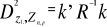
Figure 3 Principles of the calculation of the niche model that lead to probability of occurrence of a species. a. An hypothetical observation to be tested against a training set (X) composed of three observations in the space of two controlling factors. Three Euclidean distances are first calculated and then the average observed distance between the observation to be tested and the ones of the training set is assessed. b. Recalculation of the mean distance after permutation of the first observation (x1) of the training set by the observation to be tested. c. Recalculation of the mean distance after permutation of the second (x2) observation of the training set by the observation to be tested. d. Recalculation of the mean distance after permutation of the last observation (x3) of the training set X by the observation to be tested. All calculated Euclidean distances are indicated by a dashed line. The number of times the simulated mean distance is found inferior to the observed mean distance defined the probability to find the species in a region. To calculate the Mahalanobis generalized distance between each observation of the environment yi (1 = i = m) and all observations of the training set xj (1 = j = n), we used a particular form of the generalized distance, giving the distance between any observation and the centroid of an unique group (Dagnélie 1975):
With Rp,p the correlation matrix
of the standardized table (mean 0 and variance 1)
Z*, k1,p is the vector
of the differences between values of the p variables at
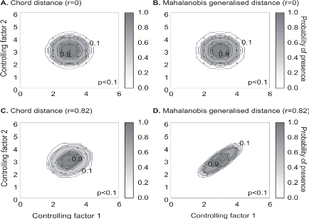
Figure 4 Fictive examples that show the better performance of the Mahalanobis generalised distance in comparison to the chord distance, justifying the choice of the distance coefficient in the ecological niche model NPPEN. First, the reference matrix is composed of 25 observations with two controlling factors. The correlation between the 2 controlling factors is null (A and B). A. Probabilities based on the chord distance (r = 0). B. Probabilities based on the Mahalanobis generalised distance (r = 0). Second, the reference matrix is composed of 13 observations with 2 parameters. The correlation between the two controlling factors is high (r = 0.82; C and D). C. Probabilities based on the chord distance (r = 0.82). D. Probabilities based on the Mahalanobis generalised distance (r = 0.82). Black circles denote the reference observations (reference matrix). High probabilities are located at the centre of the reference matrix, denoting the centre of the ecological niche (sensu Hutchinson) and probabilities <0.1 are situated outside (white colour). Maps of probability of presence are then assessed from the knowledge of the three abiotic factors and by linear interpolation in the space of the ecological niche. Figure 5 presents the modelled ecological niche for Cod (Gadus morhua L.).
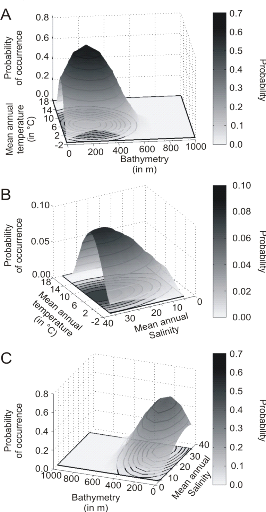
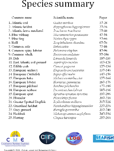
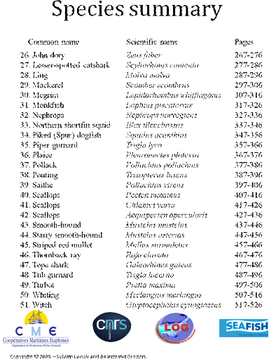
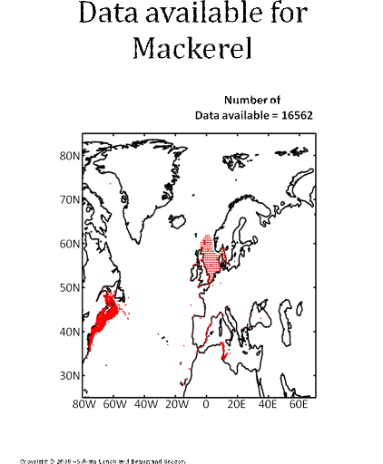
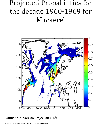
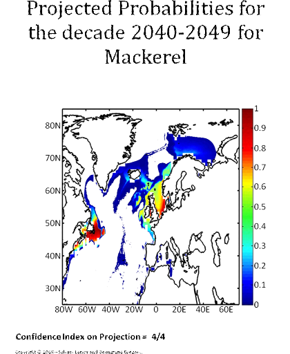
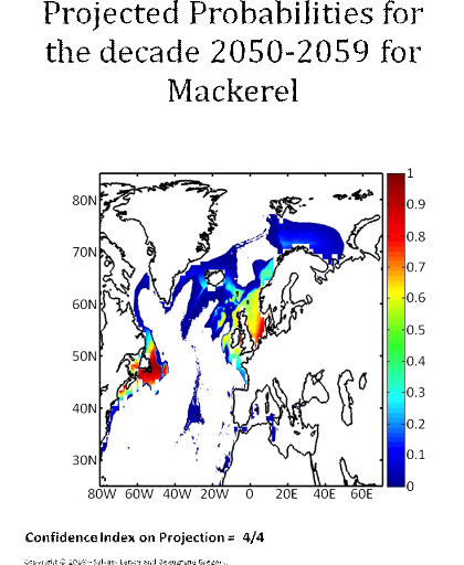
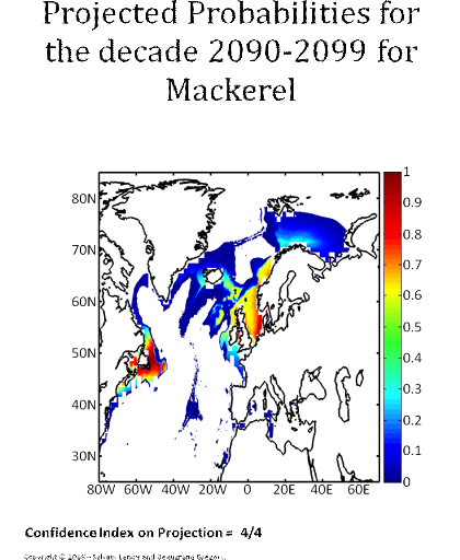
Figure 5 Realised niche (sensu Hutchinson) of the Atlantic cod. A. Probability of cod occurrence as a function of bathymetry and mean annual sea surface temperature. B. Probability of cod occurrence as a function of mean annual sea surface salinity and mean annual sea surface temperature. C. Probability of cod occurrence as a function of mean annual sea surface salinity and bathymetry. Description of the climatic atlas It was possible to apply the technique on 51 species of commercially exploited marine species (see Species Summary pages 15 and 16) The attempt to use the model on other species was not satisfactory because of a lack of occurrence data or a too incomplete coverage of the ecological niche. A confidence index was set up and used on each map in a first attempt to assess the robustness of projections. The values of the index were based on the number of presence data on which the model was applied. The index was expressed in four categories. A value of 1, 2, 3, 4 means that the model was applied on <100, 200-500, 500-1000, >1000 occurrence data, respectively. Projections are likely to be more reliable for an index of 4 (e.g. the Atlantic cod). For each of the 51 species, nine figures are attached. The first figure shows the spatial distribution of presence data used to apply the ecological niche model (Fig. 6). The total number of samples on which the model is utilised is indicated on the left of the figure (Fig. 6).
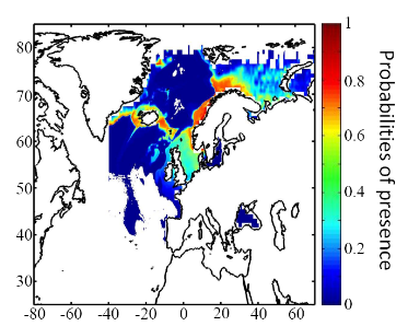
Figure 6 Spatial distribution of occurrence data for the Atlantic cod. Other maps (from two to nine) present modelled probability of presence (between 0 and 1) for the decades 1960s (observed data), 2000s, 2010s, 2020s, 2030s, 2040s, 2050s and 2090s (scenario B2). A null probability means that the physical conditions are incompatible with the presence of the species while a probability of 1 means that the presence of the species is certain. Figure 7 shows an example for the Atlantic cod (1960s).
Figure 7 Spatial distribution in the probability of presence for the Atlantic cod for the period 1960-1969. Conclusions The documents present a first outline on the potential changes in the spatial distribution of 51 commercially exploited species up to 2100 using a moderate scenario (Scenario B2, ECHAM 4). It is the result of an investigation of the relationships between climate and marine resources. Future developments should include a multimodel and a multiscenario approach to attach a better confidence interval on the projections. Two scientific papers are in preparation for submission. The delay in submitting the two papers is explained by a methodological development in 2008. The originally double approach using a parametric and a non-parametric technique has been replaced by a new technique combining strength of the two procedures: the use of the Mahalanobis technique and its test by a non-parametric procedure called MRPP and published in 2008 (Beaugrand et Helaouët 2008, Marine Ecology Progress Series; volume 363; pages 29-37). The two papers will be soon submitted in good scientific journals and are provisionally entitled: · Beaugrand G, Lenoir S, Ibañez F, Manté C (submit) Modelling the probability of occurrence of the Atlantic cod. · Lenoir S, Beaugrand G, Lécuyer E. (submit) Modelled spatial distribution of marine fish and projected modifications in the North Atlantic Ocean. References Beaugrand G (2004) The North Sea regime shift: evidence, causes, mechanisms and consequences. Progress in Oceanography 60:245-262 Beaugrand G, Helaouët P (2008) Simple procedures to assess and compare the ecological niche of species. Marine Ecology Progress Series 363:29-37 Beaugrand G, Ibanez F (2004) Monitoring marine plankton ecosystems (2): long-term changes in North Sea calanoid copepods in relation to hydro-meteorological variability. Marine Ecology Progress Series 284:35-47 Brander K (2000) Effects of environmental variability on growth and recruitment in cod (Gadus morhua) using a comparative approach. Oceanologica Acta 23:485-496 Calenge C, Darmon G, Basille M, Loison A, Jullien J-M (2008) The factorial decomposition of the Mahalanobis distances in habitat selection studies. Ecology 89:555-566 Cornelius JM, Reynolds JF (1991) On determining the statistical significance of discontinuities within ordered ecological data. Ecology 72:2057-2070 Dagnélie P (1975) Theorie et methodes statistiques, Applications agronomiques. . In: Les methodes de l'inférence statistique 2e ed, Vol 2. Presses agronomiques de Gembloux, Gembloux, p 463 Hutchinson GE (1957) Concluding remarks. Cold Spring Harbor Symposium Quantitative Biology 22:415-427 Ibañez F (1981) Immediate detection of heterogeneities in continuous multivariate, oceanographic recordings. Application to time series analysis of changes in the bay of Villefranche sur Mer. Limnology and Oceanography 26:336-349 Intergovernmental Panel on Climate Change WGI (2007) Climate Change 2007: Impacts, Adaptation and Vulnerability, Vol. Cambridge University Press, Cambridge Legendre P, Legendre L (1998) Numerical Ecology, Vol. Elsevier Science B.V., The Netherlands Levitus S (1982) Climatological Atlas of the World Ocean. In: office USGp (ed) NOAA ProfPap, Vol 13, Washington DC, p 173 Louisy P (2002) Guide d'identification des poissons marin: Europe et Méditerranée, Vol, Milan Mielke PW, Berry KJ, Brier GW (1981) Application of Multi-Response Permutation Procedures for examining Seasonal changes in monthly mean Sea-Level pressure patterns. Monthly Weather Rewiew 109:120-126 Nogués-Bravo D, Rodriguez J, Hortal J, Batra P, Araujo MB (2008) Climate Change, Humans, and the Extinction of the Woolly Mammoth. PLoS Biology 6:685-692 Smith WHF, Sandwell DT (1997) Global Sea Floor Topography from Satellite Altimetry and Ship Depth Soundings. Science 277:1956-1962 Thuiller W, Brotons L, Arau' jo MB, Lavorel S (2004) Effects of restricting environmental range of data to project current and future species distributions. Ecography 27:165-172 Woodruff S, Slutz R, Jenne R, Steurer P (1987) A comprehensive ocean-atmosphere dataset. Bulletin of the American meteorology society 68:1239-1250
CHAPITRE IV Les effets du climat sur les proies principales des oiseaux marins en mer du Nord 1. Résumé du Chapitre IV |
|


 (1)
(1) (2)
(2) (3)
(3) (4)
(4) (5)
(5) = 2.236,
  = 2.236 and
  = 1.803. The average observed distance åo is = 2.092.
The simulated distances are ås1 = 1.589, ås2
= 1.383 and ås3 = 1.140. The probability is therefore equal to
0. Observation y has environmental conditions not compatible with the species
ecological niche inferred here from 2 variables.
= 1.803. The average observed distance åo is = 2.092.
The simulated distances are ås1 = 1.589, ås2
= 1.383 and ås3 = 1.140. The probability is therefore equal to
0. Observation y has environmental conditions not compatible with the species
ecological niche inferred here from 2 variables. 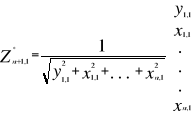 (6)
(6) (7)
(7) are the observations i of the jth variables in
Z,
are the observations i of the jth variables in
Z,  the average and
  the standard deviation of each variable j in Z.
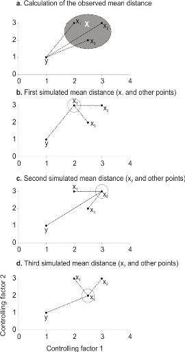
 (8)
(8) of standardized matrix Z* and the mean
  of the p variables in the standardized matrix Z*. Therefore
in Step 3, the Euclidean distance was replaced by the use of the Mahalanobis
Generalised distance. Furthermore, comparison between the chord and the
Mahalanobis generalized distance shows that when correlation between two
parameters are significantly different to 0, the ecological niche model
performs better when it is based on the Mahalanobis generalized distance
(Fig. 4).
of the p variables in the standardized matrix Z*. Therefore
in Step 3, the Euclidean distance was replaced by the use of the Mahalanobis
Generalised distance. Furthermore, comparison between the chord and the
Mahalanobis generalized distance shows that when correlation between two
parameters are significantly different to 0, the ecological niche model
performs better when it is based on the Mahalanobis generalized distance
(Fig. 4).