|

A STUDY OF THE BIRDS IN CENTRAL BANGKOK
(THAILAND) IN ORDER TO IMPLEMENT THE
BASIS OF A LONG TERM MONITORING
CAMILLE CALICIS
CO-PROMOTEURS: PR. MARIE-CLAUDE HUYNEN, PR. TOMMASO
SAVINI
TRAVAIL DE FIN D'ETUDES PRESENTÉ EN VUE DE
L'OBTENTION DU DIPLOME DE MASTER BIOINGENIEUR EN GESTION DES FORETS ET DES
ESPACES NATURELS
ANNÉE ACADÉMIQUE 2013-2014
(c) Toute reproduction du présent document, par
quelque procédé que ce soit, ne peut être
réalisée qu'avec l'autorisation de l'auteur et de
l'autorité académique de l'Université de
Liège/Gembloux Agro-Bio Tech
Le présent document n'engage que son auteur

A STUDY OF THE BIRDS IN CENTRAL BANGKOK
(THAILAND) IN ORDER TO IMPLEMENT THE
BASIS OF A LONG TERM MONITORING
CAMILLE CALICIS
CO-PROMOTEURS: PR. MARIE-CLAUDE HUYNEN, PR. TOMMASO
SAVINI
TRAVAIL DE FIN D'ETUDES PRESENTÉ EN VUE DE
L'OBTENTION DU DIPLOME DE
MASTER BIOINGENIEUR EN GESTION DES FORETS ET DES
ESPACES NATURELS
ANNÉE ACADÉMIQUE 2013-2014
I
ACKNOWLEDGEMENTS
Upon completion of this topic, I wish to sincerely thank
all those who were in any way involved in its realization.
I want first of all to thank my two co-promoters, Pr.
Marie-Claude Huynen and Pr. Tommaso Savini who allowed me to discover the world
of ornithology in the incredible city of Bangkok and I sincerely thank them for
their advices all along the redaction of the present work. Then, I would like
to thank JuanMa for his warm welcome in Bangkok, for his help concerning the
accommodation and the ways to go around the city. I don't know how I would have
done without your little red bike. Thanks also to the wonderful folks I met in
Bangkok: Mart', Lek et al., Jess, Barry and the amazing group «it's a bad
idea», particularly Gwen and Franck. Thanks to all for the sharing, the
support, the laugh...
Un tout grand merci à Marc Dufrêne et
Anaïs Gorel, car sans eux pas de stats et sans stats... pas de TFE ! Vous
vous êtes toujours rendus disponible quand j'avais des questions et je
vous en suis très reconnaissante. Merci également au professeur
Jan Bogaert pour ses pistes de discussion et à José Flahaux pour
sa relecture consciencieuse.
Ensuite, au terme de ce master en Gestion des Forêts
et des Espaces Naturels, j'aimerais remercier l'ensemble du cadre enseignant
pour les différents cours prodigués lors de ces deux
années de master. J'ai toujours apprécié la qualité
des cours et le bon équilibre entre cours magistraux et visites de
terrain. Merci de m'avoir accompagnée et transmis votre savoir !
Impossible de ne pas citer ensuite mes cokotteurs de ces
dernières années aux Déchets et à l'Auberge, avec
qui j'ai passé des moments inoubliables et sans qui la vie à
Gembloux n'aurait surement pas été la même : Romy, Alex,
Sosso, Chavroux, Pauline, Porco, Valou, Baz, Ana, Flo, Eme, Olivia, Boedts,
Sophie, Renard, Arthur ainsi que François, Justine, Angeline, BM,
Roxane, Constant, Mumu, Lewis, Val, Jey, Lio, Zara, Manon et
Hélène. Et puisque bien entendu cette vie à Gembloux ne
s'arrête pas au kot, j'ai une pensée pour mes complices du
conseil, Fanfan, Sophie, Vic', Stritsky, Baz, Schreder, Const et Francky, je
n'oublierai jamais ces merveilleux moments partagés ensemble. Un immense
merci à Charles, Clément, Camille et Olivier, mes yolo d'acolytes
de la rédaction, sans qui ce dernier mois n'aurait pas été
si gay. Et pour finir, merci à Baptiste, Amandine, Henri, Kity, Scott et
toutes les autres merveilleuses rencontres faites en ces bons vieux murs de
Gembloux !
Pour terminer je ne remercierai jamais assez mes parents
et mes trois petites soeurs, Claire, Chloë et Coraline, qui m'ont toujours
soutenue à tous les niveaux, et sans qui je ne serais pas ce que je suis
aujourd'hui ; ainsi que Thomas qui me supporte depuis presque deux ans.
Le voyage réalisé dans le cadre du
présent travail a été rendu possible grâce au
soutien financier de l'Académie de Recherche et d'Enseignement
supérieur de la Fédération Wallonie-Bruxelles, Belgique
(Commission de la Coopération au Développement)
II
ABSTRACT
Worldwide, urban sprawl, induced by current increasingly
demographic pressure, has become a prominent concern in conservation ecology.
Urban green patches are essential biodiversity hotspots in cities. Bangkok,
capital of Thailand, is among the larger cities in Asia and did not escape the
global growth of urbanization, fragmenting the green areas of its metropolis
and seeing its biodiversity collapsing like elsewhere. As part of that thesis,
we collected ornithological and environmental data into various green patches
of Central Bangkok. Indeed, the goal of this study is to investigate the
ornithological characteristics, together with the environmental factors
affecting them in order to implement the basis of a long-term monitoring of the
urban avifauna. Various indices were calculated to permit the description of
the chosen green patches' ornithological and environmental characteristics.
Then, different statistical methods were used in order to explain the previous
calculated indices' and bird communities' distribution and how the
environmental features affected them. We demonstrated that the green patch size
and water cover rate influenced the most the ornithological characteristics
indices in our study area. Several issues related to bird conservation in
Bangkok are then discussed through the main findings of this thesis. Finally,
perspective are set focusing on the fact that long-term data about birds
collected across a city can help filling the gaps caused by our lack of
understanding of the metropolitan landscapes design needs in order to better
sustain the avian fauna in the cities.
Keywords: conservation ecology, urban green
patches, birds, Bangkok, fragmentation, urban avifauna, monitoring, Southeast
Asia
RÉSUMÉ
De par le monde, la croissance urbaine, conséquence
d'une pression démographique exponentielle, est devenue une
préoccupation capitale en écologie de la conservation. Les
espaces verts urbains sont des importants centres névralgiques de
biodiversité au sein d'une ville. Bangkok, capitale de la
Thaïlande, fait partie des plus grandes villes d'Asie du Sud-Est et n'a
pas échappé à la croissance urbaine
généralisée. Les espaces verts de la métropole ont
été intensivement fragmentés et la biodiversité
s'est effondrée comme partout ailleurs. Dans le cadre de ce
mémoire, nous avons recueilli des données ornithologiques et
environnementales au sein de divers espaces verts dans le centre de Bangkok. En
effet, l'objectif de cette étude est d'analyser les
caractéristiques ornithologiques, ainsi que les facteurs
environnementaux qui les affectent afin de mettre en place les bases d'un
monitoring à long terme de l'avifaune urbaine de Bangkok. Divers indices
ont été calculés pour permettre la description des
caractéristiques ornithologiques et environnementales des espaces verts
choisis. Ensuite, différentes méthodes statistiques ont
été utilisées afin d'expliquer la distribution des indices
précédemment estimés et de définir des
communautés d'oiseaux. L'influence des caractéristiques
environnementales sur ces distributions a ensuite été
développée. Nous avons ainsi démontré que la taille
et le taux de recouvrement en eau des espaces verts sont les deux variables
environnementales qui influencent le plus la diversité ornithologique
dans notre zone d'étude. Plusieurs suggestions pour la conservation des
oiseaux à Bangkok ont ensuite été discutées
à l'aide des principaux résultats apportés par ce
mémoire. Finalement, les perspectives mettent l'accent sur l'importance
d'un monitoring à long terme de l'avifaune au sein d'une
métropole comme Bangkok.
Mots-clefs : écologie de la
conservation, espaces verts urbains, oiseaux, Bangkok, fragmentation, avifaune
urbaine, monitoring, Asie du Sud-Est
III
TABLE OF CONTENTS
I. INTRODUCTION 1
CONTEXT 1
RESEARCH QUESTIONS AND ASSOCIATED OBJECTIVES 2
WORK PLAN 2
II. LITERATURE REVIEW 3
IMPORTANCE OF BIODIVERSITY 3
II.1.1. Biodiversity in decline 3
II.1.2. The case of Southeast Asia 5
THE BIRDS STATE 6
II.2.1. Evolution of the birds of the Bangkok Area 6
II.2.2. Birds as environmental indicators 8
II.2.3. Bird monitoring 10
URBAN ECOLOGY 10
II.3.1. Cities as extinction or richness generator?
11
II.3.2. Importance of urban green spaces 11
II.3.3. Conservation keys to reduce the urban effects on
birds: state-of-the-art 12
III. STUDY AREA 14
III.1.1. General context 14
III.1.2. Climate and Altitude 15
III.1.3. Land use 16
IV. METHODOLOGY 18
VEGETATION PATCHES SAMPLING 18
RAW DATA COLLECTION 20

IV.2.1. Ornithological surveys 20
IV.2.2. Environmental surveys 23
DEFINITION AND CALCULATION OF THE VARIABLES 25
IV.3.1. Ornithological variables 25
IV.3.2. Environmental variables 26
DATA ANALYSIS 28
IV.4.1. Ornithological distribution analyses 28
IV.4.2. Ornithological communities analysis 30
IV.4.3. Environmental characteristics analyses 33
IV.4.4. Environmental explicatory factors of the
ornithological distribution analysis 34
V. RESULTS 36
ORNITHOLOGICAL DISTRIBUTION ANALYSIS 36
V.1.1. Species Richness 37
V.1.2. Abundance Distribution 41
V.1.3. Biotic homogenization index 43
ORNITHOLOGICAL COMMUNITIES ANALYSIS 45
V.2.1. Structure of the Ornithological data 45
V.2.2. Indicator Species 46
ENVIRONMENTAL CHARACTERISTICS 47
V.3.1. Correlations matrix of the environmental variables
47
V.3.2. Principal Component Analysis of the environmental
variables 48
ENVIRONMENTAL FACTORS EXPLAINING THE ORNITHOLOGICAL DISTRIBUTION
51
V.4.1. Indirect gradient analysis 51
V.4.2. Generalized linear models 52
V.4.3. Direct gradient analysis 54
VI. V
DISCUSSION 56
HOW IS THE AVIFAUNA CHARACTERIZED AND DISTRIBUTED INTO GREEN
PATCHES SITUATED IN THE CENTER OF THE BANGKOK
METROPOLIS? 56
HOW DO THE ENVIRONMENTAL PARAMETERS OF THOSE GREEN PATCHES
INFLUENCE THE BIRD DISTRIBUTION? 58
IMPLICATIONS FOR CONSERVATION 61
STUDY LIMITS 60
VI.4.1. Limits regarding the study scope 60
VI.4.2. Limits concerning the bird data collected 60
VI.4.3. Limits due to the choices of environmental indices
61
VII. CONCLUSION AND PERSPECTIVES 61
VIII. BIBLIOGRAPHY 63
VI
LIST OF ABBREVIATIONS
AICc - small sample size Akaike's Information Criterion
BMA -Bangkok Metropolitan Administration
CSI-Community Specialization Index
e.g.- exempli gratia (for example)
GIS - Geographic Information System
GLM - Generalized linear models
GPS - Global Positioning System
i.e. - id est (that is)
IBA - Important Bird Area
IBT-Island Biogeography Theory
PCA-Principal Component Analysis
PCoA- Principal Coordinate Analysis
Pers. obs. - Personal observation
RDA - Redundancy Analysis
RSE - Residual Standard Errors
SSI-Species Specialization Index
VII
LIST OF FIGURES
FIGURE 1: ORGANIZATION OF THE THESIS RESEARCH QUESTIONS AND
OBJECTIVES 2
FIGURE 2: FUNCTIONS PROVIDED BY THE ECOSYSTEM 4
FIGURE 3: SPECIES RICHNESS AND ENDEMISM IN THE FOUR
BIODIVERSITY HOTSPOTS OF SOUTHEAST ASIA.) 5
FIGURE 4: BIRD SPECIES DISTRIBUTION INTO THE IUCN RED LIST
CATEGORIES. 7
FIGURE 5: LOCALIZATION OF THE STUDY AREA. 14
FIGURE 6: BANGKOK CLIMATE CHART 15
FIGURE 7: MAP OF THE PATCHES SAMPLED IN CENTRAL BANGKOK 20
FIGURE 8: DIGITALIZATION OF THE LAND COVER 23
FIGURE 9: METHOD USED FOR THE ORNITHOLOGICAL COMMUNITIES
ANALYSIS 31
FIGURE 10: CUMULATIVE RICHNESS CURVES FOR THE PATCHES NO.3 AND
NO.8 38
FIGURE 11: MAP OF THE SPECIES RICHNESS PER PATCH IN THE STUDY
AREA 39
FIGURE 12: AMOUNT OF SPECIES CHARACTERIZED BY DIFFERENT
DISTRIBUTION (NUMBER OF RECORDS) IN THE STUDY AREA. 40
FIGURE 13: MAP OF THE SHANNON INDEX OF DIVERSITY PER PATCH IN
THE STUDY AREA 41
FIGURE 14: AMOUNT OF SPECIES INDIVIDUALS CHARACTERIZED BY
DIFFERENT RELATIVE DENSITIES IN THE STUDY AREA. 42
FIGURE 15: COMMUNITY SPECIALIZATION INDEX
(CSI) DISTRIBUTION IN THE STUDY AREA 43
FIGURE 16: COMPARISON OF THE DESCRIBING PARAMETERS OF THE
ORNITHOLOGICAL DATA CALCULATED IN THE 25 PATCHES STUDIED 44
FIGURE 17: DENDROGRAM FORMED OUT OF THE WARD'S MINIMUM
VARIANCE METHOD 45
FIGURE 18: FACTORIAL DESIGN CREATED WITH THE TWO FIRST AXIS OF
THE PCOA CONCERNING THE ABUNDANCE DATA 46
FIGURE 19: REPRESENTATION OF THE ENVIRONMENTAL VARIABLES IN
THE PEARSON AND SPEARMAN CORRELATION CIRCLES FORMED BY
THE TWO FIRST AXES OF THE PCA 49
FIGURE 20: FACTORIAL DESIGN CREATED WITH THE TWO FIRST AXIS OF
THE PCA CONCERNING THE ENVIRONMENTAL DATA 50
FIGURE 21 REPRESENTATION OF THE ENVIRONMENTAL VARIABLES
TOGETHER WITH THE ORNITHOLOGICAL DESCRIPTIVE PARAMETERS IN THE
PEARSON AND SPEARMAN CORRELATION CIRCLES FORMED BY THE TWO
FIRST AXES OF THE PCA. 51
FIGURE 22: RESIDUALS PLOTS OF BEST GLM 53
FIGURE 23: RESIDUALS PLOTS OF BEST GLM 54
FIGURE 24: REPRESENTATION OF THE SPECIES ABUNDANCE AND
ENVIRONMENTAL VARIABLES IN THE PLOT FORMED BY THE TWO FIRST AXES
OF THE RDA 55
VIII
LIST OF TABLES
TABLE 1: SYNTHESIS TABLE BRINGING CONSERVATION KEYS IN ORDER TO
ALLEVIATE THE EFFECTS OF URBANIZATION ON BIRDS. 13
TABLE 2: AREA OF MAIN LAND USES IN BANGKOK 16
TABLE 3: LAND COVER TYPE DESCRIPTION 24
TABLE 4: CRUDE ORDINAL SCALE OF ABUNDANCE DEDUCTED FROM THE
ENCOUNTER RATE DATA 25
TABLE 5: PARAMETERS DEFINING THE PATCHES 26
TABLE 6: LANDSCAPE INDICES 27
TABLE 7: OBSERVED AND ESTIMATED REAL RICHNESS WITHIN THE PATCHES
37
TABLE 8: SPECIES SELECTED VIA THE INDVAL METHOD AS BEING
SIGNIFICANTLY ASSOCIATED TO A GROUP OF SITES 47
TABLE 9: PEARSON AND SPEARMAN CORRELATION COEFFICIENTS BETWEEN
THE ENVIRONMENTAL VARIABLES AND THE TWO AXES OF THE
PCA. 49
TABLE 10: PEARSON AND SPEARMAN CORRELATION
COEFFICIENTS BETWEEN THE ORNITHOLOGICAL VARIABLES AND THE TWO AXIS OF THE
PCA. 51
TABLE 11: GENERAL LINEAR MODELS AND SUMMARY STATISTICS FOR
ORNITHOLOGICAL VARIABLES 52
TABLE 12: PEARSON AND SPEARMAN CORRELATION COEFFICIENTS BETWEEN
THE ENVIRONMENTAL VARIABLES AND THE TWO AXES OF THE
RDA 55
IT CAN SEEM WEIRD TO STUDY THE BIRD IN A CITY
LIKE
BANGKOK METROPOLITAN...
YOU COULD THINK THAT THERE ARE ONLY PIGEONS
THAT
EVERYONE TRIES TO GET RID OF...
...BUT THIS THESIS WILL SHOW YOU THAT BIRD IS
AN
INCREDIBLE TAXA IN WHICH A LOT OF SPECIES
MANAGE TO ADAPT TO EVEN THE
NASTIEST HABITAT
I. INTRODUCTION
1
CONTEXT
Bangkok, capital of Thailand, is among the larger cities in
Asia with an estimated unofficial population of more than 10 million people
(THAIUTSA et al., 2008) and did not escape the global growth of urbanization,
fragmenting the green areas of its metropolis and seeing its biodiversity
collapsing like elsewhere in Southeast Asia (SODHI et al., 2004; SODHI and
BROOK, 2006).
Urban ecology actions are more urgent now than they have ever
been, especially in developing countries that contain some of the world's
largest metropolitan areas. According to the World Urbanization Prospects
(UN, 2012), Asian cities host about half of the urban population of the
world, with this number expected to increase by 1.7 times over the next four
decades.
The Southeast Asian region is characterized by four
biodiversity hotspots. When coupling that high biodiversity with the high human
population density, the region comes to be one of the most endangered
biodiversity hotspots where demographic and economic pressures have led to
extensive conversion of forests and overexploitation of coastal resources
(WILLIAMS, 2012).
Studies of the avian fauna in metropolitan areas show that
cities generally remain hostile places to most native bird species. However,
these areas in which people live, work and play could take on an increasingly
vital role in sustaining biological diversity (TURNER, 2003). Wildlife
diminution rates can only be arrested by reconciling activities in production
landscapes (agriculture and urban) with the conservation of nature (ROSENZWEIG,
2003). Long-term data about birds collected across a city can help filling the
gaps caused by our lack of understanding of the metropolitan landscapes design
needs and allow to better sustain the avian fauna in the cities (TURNER,
2003).
Two features of importance will be especially highlighted
throughout this master thesis. First, in a general context of decline and
homogenization of populations of urban birds (DEVICTOR et al., 2008; MCKINNEY,
2006; SAX and GAINES, 2003), it is a key applied issue to understand and to
predict their distribution and persistence in the modern, fragmented landscapes
humans created. Second, urban green spaces are an essential foundation for a
healthy population, a healthy economy and for ecological balance in any city
(BOLUND and HUNHAMMAR, 1999; WHO, 2008) and it is thus essential to predict how
their environmental composition affects birds to better understand the value of
those urban green spaces (KOSKIMIES, 1989).
The impact of the intensive environmental changes on the avian
fauna of Bangkok haven't been studied yet and long-term data on multi-species
distribution are inexistent (ROUND, 2008). Thereby, a first step would be to
study the distribution of existing avian fauna in Bangkok to establish a
long-term monitoring and set priorities for its long term conservation.
2
RESEARCH QUESTIONS AND ASSOCIATED OBJECTIVES
This thesis reports on surveys of the avifauna within various
vegetation patches of Bangkok with the aim of providing basis for long term
monitoring actions.
In order to best achieve the stated goal, we centered our work on
two principal research questions and the ensuing objectives (Figure 1).
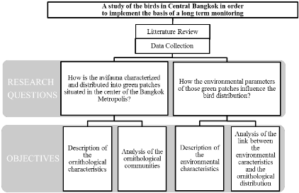
Figure 1: Organization of the thesis research questions and
objectives
After having achieved the present objectives, the basis to
implement a long term monitoring will be set and a discussion will be oriented
to bring preferences for Bangkok avifauna conservation.
WORK PLAN
This master thesis is divided into 7 sections. To put things
into context, the first two sections consist in a brief introduction, followed
by a literature review supporting the general framework of the study. Then, the
third section will describe the area in which the study was realized. Section 4
will present the methodology and the analyses that we used in order to reach
the objectives previously described. Section 5 will then show the results of
the analyses and sections 6 and 7 will discuss and conclude the results
obtained, finalizing with the perspectives regarding the long-term
monitoring.
II. LITERATURE REVIEW
This section aims at setting the general context of this
study, using what the literature can offer so far. It will start by a brief
recall of the actual worldwide biodiversity crisis, focusing then more on the
description of the situation in Southeast Asia. Afterwards, we will provide an
overview of the bird taxa situation, starting with the general trend of the
evolution of their populations in Bangkok. We will also show the bird's
importance as environment indicators as well as the need of monitoring them to
explain environmental changes. We will next have a look at the effect of
urbanization on birds and the importance of urban green areas, finally giving
conservation clues from studies made in other cities.
IMPORTANCE OF BIODIVERSITY
«La caractéristique la plus merveilleuse de
notre planète est la présence de la vie et
la
caractéristique la plus incroyable de la vie est sa
diversité1!» (BEUDELS, 2013)
II.1.1. Biodiversity in decline
The term «biodiversity» is a contraction of
«biological diversity» and was defined by the Convention on
Biological Diversity (UNCED, 5th of June 1992) as:
«The variability among living organisms from all sources including,
inter alia, terrestrial, marine and other aquatic ecosystems and the ecological
complexes of which they are part: this includes diversity within species,
between species and of ecosystems.» First, this term was closely
related to nature conservation but has been then associated with more
functional and utilitarian notions, especially after the publication of the
MILLENNIUM ECOSYSTEM ASSESSMENT (MEA; 2005) which connected interactions
between people, biodiversity and ecosystems.
Indeed, despite the fact that most humans consider themselves
above everything, the biodiversity that surrounds them is indispensable to
their survival. In fact, the changes in human condition leads to changes in
biodiversity and in ecosystems and thus, have an ultimate effect on the
services provided by the ecosystems which make biodiversity and human
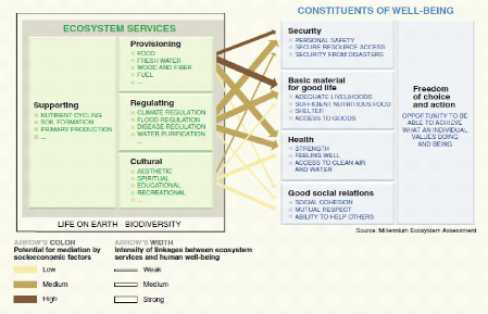
well-being entirely linked together (MEA, 2005). Species conservation is not
only giving the species the right to exist, it also adds value to human's life
by providing supporting, provisioning, regulating and cultural functions as
shown in Figure 2.
3
1 «The most wonderful characteristic of our
planet is the presence of life and the most incredible characteristic of life
is its diversity»
4
Figure 2: Functions provided by the ecosystem (MEA,
2005)
Currently, biodiversity is unequivocally declining and some
authors even speak about a «6th extinction crisis» (LEAKEY
and LEWIN, 1999; MEA, 2005). If the extinction of a species is indeed a natural
process (75 to 95% of all species that have ever existed are now extinct),
today's biodiversity is disappearing at a 100 to 1000 times higher rate than
the mean natural extinction rate that occurred during the fifth previous
extinctions. So, the concern is not about the occurrence of extinctions, but
rather about the acceleration of the extinction process: if nothing is done,
50% of the actual species will have disappeared before the end of the
XXIst century (LEAKEY and LEWIN, 1999) and a world of pests and
weeds will remain.
Nowadays, the challenge is to implement a sustainable
development ensuring the social and economic viability of human societies while
respecting the ecosystems (BROWN, 2001). Protecting those ecosystems requires a
good basic knowledge of them, which can be improved by scientific research. As
shown before, biodiversity is a quite nebulous and extremely large concept.
Nonetheless, it must unconditionally be quantified in order to reach political
decisions or to implement management measures or to reach a priority for
actions. An important difficulty in quantifying biodiversity is that it is a
multifaceted concept (PURVIS and HECTOR, 2000) and it must be done at a defined
scale and with a defined and refocused objective (HOSTETLER, 1999).
5
II.1.2. The case of Southeast Asia
Although Southeast Asia (Brunei, Cambodia, Indonesia, Laos,
Malaysia, Myanmar, the Philippines, Singapore, Timor-Leste, Thailand, and
Vietnam) incorporates four biodiversity hotspots (BRIGGS, 1996; SODHI et al.,
2004; WILLIAMS, 2012) (Figure 3), the region faces several key social,
scientific and logistical conservation challenges.
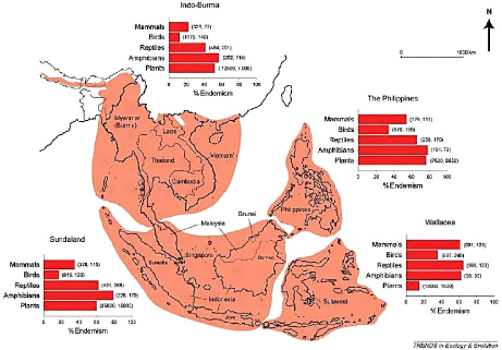
Figure 3: Species Richness and endemism in the four
biodiversity hotspots of Southeast Asia. The red bars represent the percentage
of species endemic to the respective hotspot. Numbers in parentheses represent
total and endemic species known to science, respectively (SODHI et al.,
2004)
Among all the world's tropical regions, Southeast Asia has the
highest rate of habitat lost with a deforestation rate four times higher than
elsewhere in the world (FAO, 2012). This fact is alarming knowing that compared
to the other tropical regions, Southeast Asia has the highest mean proportion
of country-endemic bird (9%) and mammal species (11%) as well as the second
highest rate of country-endemic vascular plant species (25%) (SODHI et al.,
2009).
The current major threats to biodiversity in Southeast Asia
are predominantly from socioeconomic origin; including population growth,
poverty, chronic shortage of conservation resources and corrupt national
institutions. Hence, as the regional societies of Southeast Asia attempt to
match
6
the living standards of developed nations, environmental
issues are inexorably marginalized (SODHI et al., 2004; SODHI and BROOK, 2006).
This is supported by the fact that the economic constraints are much larger in
the developing countries like Thailand, than in North America or Europe and
therefore it is difficult to find money for environmental management when basic
needs and poverty are an immediate bigger concern (FRASER, 2002).
Lastly, research on Southeast Asian biodiversity over the past
20 years has been neglected in comparison to other tropical regions (SODHI and
BROOK, 2006). Indeed, it appears that there is a shortage of local scientists
conducting rigorous conservation biology research in Southeast Asia, with the
current work dominated by descriptive work, mostly inventories (SODHI and LIOW,
2000). These trends are disturbing and the consequence can be even more severe
for that region because of the habitat destruction that occurred during the
last century. Some solutions were brought by SODHI and LIOW (2000) to improve
the quality of conservation biology research of Southeast Asia. They range from
an increased accessibility to the international conservation biology journals
to the start of more multinational collaborative projects, more rigorous funds
for long-term research, education of local scientists in research design to
reach the standards in order to be published in international journals ...
THE BIRDS STATE
«Birds are among the best known parts of the Earth's
biodiversity. But nevertheless soundly quantified knowledge is far from
complete for most species and regions.» (BIBBY et al., 1998a)
The bird taxa did not avoid the general biodiversity decline,
and indeed, according to the IUCN Red List of Threatened Species
(IUCN, 2013), 12% of the world avian species are now threatened. For a
long time, the major threats for the birds were the variability of climatic
events and their effect on vegetation. Those have been lately supplanted by the
human impacts on the environment. During the last centuries, the pressure
humans put on nature increased substantially with the intensification of
urbanization and agriculture that generates the vanishing of many
ecosystems.
II.2.1. Evolution of the birds of the Bangkok
Area
The study of avian fauna of Southeast Asia reveals alarming
trends: if the region hosts the highest mean proportion of endemic bird species
at a national level, it also has the highest mean proportion of threatened bird
species of all tropical regions. Despite this, the avifauna of Southeast Asia
has been one of the least studied in the tropics (SODHI et al., 2006).
Thailand, as a country, holds 971 bird species (IUCN, 2013).
925 are native bird species while 1 has been introduced (Columbia
Livia), 40 are vagrant species and 5 species are still uncertain data.
Figure 4 shows a pie chart of Thailand bird species distribution through the
IUCN Red List Categories.
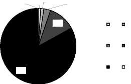
804
10 13
2 28
114
VU NT
CR EN
LC DD
7
Figure 4: Bird species distribution into the IUCN Red List
Categories. CR= Critically Endangered, EN=
Endangered,
VU=Vulnerable, NE=Near
Threatened, LC= Least Concerned, DD= Data
Deficient (Values sources: IUCN, 2013)
PHILLIP ROUND (2008) in his book, «The birds of the
Bangkok area», reviewed the birds of the Central Plain of Thailand.
He also put together existing behavioral, life-history and ecological data on
birds around Bangkok. The following paragraphs give a short summary of the
evolution of the avian state in Bangkok that ROUND (2008) developed in the
introduction of his book.
Once, the Central Plain held a bird and mammal mega fauna that
vanished because of the high rate of destruction due to large-scale historical
transformations in Thailand. Unfortunately, historic surveys of the wildlife of
Bangkok are poor. Some old records inform us about the previous presence of
ibises, pelicans, adjutants, vultures and birds characteristic of open forests.
All those species are not there anymore, only smaller and ecologically tolerant
birds of forests and secondary growth persisted until the seventieth century.
The gradual decrease in the number of resident bird species in the Central
Plain is clear and keeps happening since the intensification of agriculture and
the spread of housing and industry. The Asian Economic Crisis, from
mid-1997th onwards, gave the environment of the Chao Phraya Delta a
brief respite from land speculation and uncontrolled development. However,
today's economy is once again booming with all that is involved and no
additional environment safeguards are put in place.
Nowadays, Bangkok's urban green areas are sparse compared with
many other capitals and only the most ecologically tolerant species still
survive well in inner city gardens and parks (Coppersmith Barbet, Common Iora,
Pied Fantail, Oriental Magpie Robin, Streak-eared Bulbul, Common Tailorbird,
Scarlet-backed Flowerpecker, Brown-throated Sunbird and Olive-backed Sunbird).
Introduced bird species are also often seen in the city while they escape their
cages, like the White-Crested Laughingthrush or the Red-Breasted Parakeet.
Still, many birdwatchers are constantly amazed at how many species of birds
they are able to see in the concrete jungle of Bangkok (pers. obs.).
8
Parks are of great importance in order to provide habitats for
the birds but most of Bangkok's public parks have tended to be too deeply
manicured to support many species. Native vegetation is disappearing and even
water bodies are polluted with herbicides to prevent the colonization of
aquatic vegetation. Though, the direct widespread impacts of pollution can't be
estimated because of the absence of any systematic monitoring of the levels of
toxic pollutants in birds.
An initiative came from the Bird Conservation Society of
Thailand, which explored the possibility to implement an urban bird reserve in
eastern Bangkok together with the Bangkok Metropolitan Administration (BMA).
Regrettably, this effort fizzled out due to a change of BMA governor.
The previous trends highlighted by ROUND (2008) made that
BirdLife international decided in 2004 to consider the inner gulf of Thailand
(100,000 ha), including the Bangkok Metropolis, as an Important Bird Area (IBA)
in order to control the over-exploitation of natural resources and promote
compatible forms of land use across the whole area. The function of the IBA
program worldwide is «to identify, protect and manage a network of
sites that are significant for the longterm viability of naturally occurring
bird populations, across the geographical range of those bird species for which
a site-based approach is appropriate» (CHAN et al., 2004). However,
this applies more to the coastal area where the actions are concentrated than
to the Metropolis situation.
II.2.2. Birds as environmental indicators
As there is much concern today about environmental changes, it
is essential to know how those changes affect wildlife, and birds offer a great
value as biological and environmental indicators (BIBBY, 1999; GOTTSCHALK et
al., 2005).
In fact, they reflect well the global health of the
surrounding biodiversity because they often have a high position in the trophic
chain and also because they respond fast to landscape modifications. They are
among the most conspicuous (POMEROY, 1992), indeed, compared to other animal
taxa, birds are relatively easy to detect, identify and survey. They have been
subject to numerous studies, especially in Europe and America and therefore
their eco-ethology is generally well documented. Bird diversity was also found
to be correlated with the diversity of other taxa (BLAIR, 1999, SATTLER et al.,
2010) which means that they may be reliable indicators of the overall
biodiversity. Additionally, many studies have shown that birds are particularly
useful to detect unexpected changes, for example, due to the pesticides, as
RACHEL CARSON (1962) denounced with her famous book, «Silent
spring».
If birds are good environment indicators, it is also and
primordially because of the relationship between a bird and its habitat. FULLER
(2012) presents a good and recent synthesis of the multiple publications
concerning the processes of habitat selection by birds and the following
section is a brief description of these.
The habitat is the environment in which an individual lives,
including biotic and abiotic features as climate, microclimate, soil type,
topography, plant species and vegetation structure as well as the other animal
species living in the same environment. The use of a habitat by a bird, meaning
the way it uses the free spaces and the various resources it contains, differs
obviously between every species but also in between the same species, for
example, with the age or the sex of the animal. For birds in particular, the
factors affecting the habitat evolve considerably along the year, especially
for the migrant species or for the sedentary birds living in latitudes where
the seasons are highly contrasted. Usually, it is during the breeding time that
birds show the severest association with one habitat.
Mechanisms explaining how a bird chooses its habitat are
better and better known. The notions of «ultimate factors» and
«proximate factors» in habitat selection have been highly developed
in the past (HILDÉN 19652, cited by FULLER, 2012) and are
still universal.
- Ultimate factors: Basic factors defining the choice
of habitat through its fitness potential (e.g. food-supply, shelter
availability, territory space, structural and functional characteristics, other
species...)
- Proximate factors: Immediate signs or stimuli that
are not automatically of fitness value (e.g. landscape and microhabitat
features, vegetation density or height, microhabitats or functional sites like
song posts...)
Therefore, in order to allow the birds to select habitat that
offers the best fitness, the «proximate factors» have to be
correlated with the «ultimate factors». This is all the more
important when habitat' quality can't be determined at the time the bird chose
is territory, especially in the case of migratory birds which need to quickly
select an area to stop.
Furthermore, the spatial scale is important as well to
understand how birds select their habitat. Indeed, birds being very mobile
animals and generally in need of several types of resources, the mechanisms of
selection of their territories are often spatially hierarchized. Certain
species start identifying a potential habitat using the general landscape'
characteristics, perceived by flying over for example. Then, the exact location
of their territory can be elected as a result of a finer scale' analysis. For
example, the initial selection of a territory is based on the most common
resource but the refinement to the final location will be done on the most
limiting resource. In this case, the bird starts to take an interest at a finer
scale and then starts checking other factors at a coarser scale. The spatial
process encountered at various scales is all equally determinants in order to
explain the choice of a habitat by a bird.
9
2 HILDÉN O., 1965. Habitat selection in birds-a
review. Ann. Zool. Fenn., 2, pp. 53-75.
10
II.2.3. Bird monitoring
Birds are also useful for monitoring and incorporating
cumulative changes over long periods of time (BIBBY, 1999; KOSKIMIES, 1989).
Birds counts conducted in a systematic and consistent way can provide an
early-warning system in order to assess the health of an ecosystem. This is
essential for the authorities to ensure that development is truly sustainable
(POMEROY, 1992).
According to KOSKIMIES (1989), monitoring corresponds to
«continuous and regular quantitative research using standardized
methods, which reveal changes in the abundance and ecology of birds».
In order to be well studied, the changes need to be clearly divided between
those caused by human activities and those caused by the natural dynamics like
the climatic changes, the geological processes or the biological evolution.
Indeed, the last one affects the bird populations much more slowly than the
human-caused ones. The first advantage of biological monitoring in opposition
with non-biological monitoring is that environmental changes are detectable,
especially for those that can't be observed or forecasted by the measurement of
a set of pre-selected physical or chemical parameters. The second advantage is
that biological monitoring makes it possible to detect and monitor cumulative
and non-linear consequences of various environmental changes acting
simultaneously. An integrated monitoring can allow to study cause-effect
relationships which are truly important in order to decide the actions to be
taken (KOSKIMIES, 1989).
The more changes the environment undergoes, the more it
becomes necessary to learn how to manage it in order to take care of species
conservation. Many cases need action but without precise data on numbers or
trends, no useful recommendation for management action can be made.
Furthermore, there is a need for a large ecological knowledge in many
situations because we are continually changing our environment and in so doing,
the birds with which we share it are inexorably affected (POMEROY, 1992)
In Thailand, assessment of the effect of various construction
projects on biodiversity consists of little more than some unauthenticated
lists of birds, mammals, or other taxa (ROUND, 2008). Indeed, a regrettably
usual scheme in the case of birds is the statement that the impacts of their
habitat damages will be minimal because the birds are able to fly to other
areas.
URBAN ECOLOGY
«The effect of urbanization can be immense, yet our
understanding is rudimentary»
(CHACE and WALSH, 2006).
Rapid urbanization has turned out to be one of the major
concerns in conservation ecology (MILLER and HOBBS, 2002) and can be justified
by the fact that the world urban population is expected to increase by 72 per
cent by 2050 (UN, 2012). Moreover, cities occupy less than 3% of the global
terrestrial surface, but account for 78% of carbon emissions, 60% of
residential water use, and
11
76% of wood used for industrial purposes (BROWN, 2001). Still,
the intensifying conflict between the economy and the ecosystem of which it is
part is evident and undeniably, urbanization will keep having a significant
impact on the ecology at local, regional and global scales (SINGH et al.,
2010).
II.3.1. Cities as extinction or richness
generator?
Uncontestably, urbanization and anthropogenic activities
intensification in the landscapes change the ecosystem at many levels which
lead to the homogenization of habitat structure and composition (FORMAN, 1995).
For example, the urban sprawl is made of redundant artificial infrastructures
that homogenize the urban landscape (MCKINNEY, 2002; 2006). This has a major
negative impact on biodiversity and on the ecosystem capacity to ensure the
expected services (FORMAN, 1995).
However, urban areas seem characterized by a more important
species abundance than suburban areas for some biological groups (KÜHN et
al., 2004; ARAÚJO, 2003; NIELSEN et al., 2013). Indeed, some species
find alternative ecological niches in the cities and are able to develop
important populations like it is the case for the well-known Columbia Livia
(Rock Pigeon). Urban land-uses represent ideal habitats for the
demographic explosion of those urban-exploiter species, able to use the
abundant food resources associated to human litter (ORTEGA-ÁLVAREZ and
MACGREGOR-FORS, 2009). Therefore, many studies claim the threat of the massive
disturbances created by city growth on the habitat of native species (CONOLE
and KIRKPATRICK, 2011; DEVICTOR et al., 2008; MCKINNEY, 2006). Indeed, those
disturbances create a new habitat for few widespread non-native species that
are easily adapting to urban conditions and enrich the local biodiversity while
the global diversity is decreasing subsequently to the extinction of
non-adapting local species (SAX and GAINES, 2003).
Those apparent contradictions probably result from differences
between the geographic scales used, sampling bias, different contexts or else
different biological responses (MACDONNELL and HAHS, 2008). Identifying the
proximal factor of the urban diversity is relatively difficult as well as
studying urbanizations gradients and biological response that are far from
being linear (MACDONNELL and HAHS, 2008). Nevertheless, natural populations'
extinction in the most urbanized parts of a city seems well established,
especially in the new growth tropical cities. The geographic layout of the
urban biodiversity hotspots is fundamental and there is a major lack of
protected areas in the urban environment (BASTIN and THOMAS, 1999,
SANDSTRÖM et al., 2006).
II.3.2. Importance of urban green spaces
The «urban green spaces» comprises all urban parks,
forests and related vegetation (SINGH et al., 2010); even cemeteries can be
considered so (LUSSENHOP, 1977). According to the WHO (2008), at least 9
m2 of urban green space per capita is recommended to alleviate
undesirable
12
environmental effects and provide other benefits like a
healthy population and a sustainable economy in any city (KUCHELMEISTER, 1998).
However, the amount of required open green spaces per city dweller has remained
controversial (SINGH et al., 2010). Those amounts have been estimated for some
developing countries cities like Seoul that has 14 m2 of urban green
per capita (KUCHELMEISTER, 1998), Singapore, 10 m2 (CHOW and ROTH,
2006), Beijing, 6 m2 (DEMBNER, 1993), Mexico City, 1.9m2
(DELOYA, 1993) and New Delhi, 0.12 m2 (KUCHELMEISTER, 1998).
This is quite alarming while knowing that within municipal
limits of 26 large European cities, the average of urban green space is
estimated at 104 m2 per inhabitant (KONIJNENDIJK, 2003). Indeed,
urban green spaces are increasingly critical to healthy cities (WHO, 2008),
even more in developing countries that include some of the world's biggest
metropolitan areas and have the greater rate of urbanization (UN, 2012).
A functional network of urban green spaces can contribute to
ecological diversity in a city (SANDSTRÖM et al., 2006). The major
benefits of green spaces are (LAGHAI and BAHMANPOUR 2012):
- Assimilation of Carbon dioxide and other toxic gases as well as
Oxygen production
- Regulation and improvement of cities climate
- Noise pollution reduction and improvement of human
well-being
- Prevention of water and wind erosion
- Diminution of floods hazard
- Prevention of unsuitable urban development and increase of the
beautifulness of the city
Green spaces perform important functions and services
worldwide (NIELSEN et al., 2013), their development has the potential to
moderate the adverse effects of urbanization in a sustainable way, making
cities more attractive to live in, reversing urban sprawl, and decreasing
transport demand (DE RIDDER et al., 2004).
II.3.3. Conservation keys to reduce the urban effects on
birds: state-of-the-art
Despite high stress ensuing from urban life features such as
noise (KATTI and WARREN, 2004), air and soil pollution (MCKINNEY, 2002; ROUND,
2008) and high densities of domestic predators (ANDERIES et al., 2007; SORACE,
2002), urban areas throughout the world are characterized by high food resource
abundance and high avian population densities but as developed before, lower
species diversity is generally observed (MARZLUFF et al., 2001).
Many studies have attempted to determine the impacts of
urbanization on birds worldwide together with solutions in order to alleviate
the damages done to bird communities. Table 1 brings a state-of-the art giving
conservation keys brought from multiple scientific studies.
13
Table 1: Synthesis table of the publications bringing
conservation keys in order to alleviate the effects of urbanization on
birds.
Conservation Keys Reference
ON-FIELD ACTIONS
|
Creating park connectors, enhancing structurally diverse native
vegetation in streetscapes
|
SANDSTRÖM et al., 2006; SODHI et al., 1999; WHITE et al.,
2005
|
|
Enhancing habitat diversity and resource availability for the
avifauna within the urban green spaces (e.g. shrub and tree planting, water
restoration and increasing vegetation diversity)
|
CLERGEAU et al., 2002; FERNÁNDEZ-JURICIC and
JOKIMÄKI, 2001;
IMAI and NAKASHIZUKA, 2010; KHERA et al., 2009; LIM and SODHI,
2004; ORTEGA-ÁLVAREZ and MACGREGOR-FORS , 2009; SANDSTRÖM et al.,
2006; SAVARD et al., 2000
|

Identifying the areas of high conservation interest
BLAIR, 1999;
RAMALHO and HOBBS, 2012; SODHI et al., 2004
SAX and GAINES, 2003;
Integrating social and socio economic processes (e.g. poverty
alleviation, public SODHI et al., 2004;
education, work with various stakeholders) SODHI et al.,
2006;
TURNER, 2003;
|
Promoting the preservation and restoration of local indigenous
species (identification, conservation and creation of attributes of the urban
landscape that best protect indigenous bird assemblage, diversity and
structure)
|
CHACE and WALSH, 2006; CONOLE and KIRKPATRICK, 2011; LIM and
SODHI, 2004; MCKINNEY, 2006;
ORTEGA- ÁLVAREZ and MACGREGOR-FORS, 2009; SAX and GAINES,
2003; VAN TURNHOUT et al., 2007
|
RESEARCH DESIGNS
ANDRÉN, 1994;
Using the habitat island ecological theory as a research
framework for the FAHRIG, 2003;
management and conservation of urban birds
FERNÁNDEZ-JURICIC and
JOKIMÄKI, 2001

Understanding better the degree to which species respond to
local environmental conditions and landscape patterns
FAHRIG, 2003; FULLER, 2012; GALITSKY, 2012
Identifying species diversity changes across time at
multi-scales
|
MA et al., 2012;
SAVARD et al., 2000; SAX and GAINES, 2003;
WHITE and HURLBERT, 2010
|

Using satellite-based remote sensing together with bird data in a
GIS environment
GOTTSCHALK et al., 2005
in order to assess causal effects in species- environment
relationships
Using a Community Specialization Index for measuring
functional homogenization on both local and global scales across time
DEVICTOR et al., 2008
Greater understanding of people and wildlife interactions SAVARD
et al., 2000
14
III. STUDY AREA
We carried out the study in Bangkok, Thailand's capital, both
a city and a province. The metropolis of Bangkok covers a 1,568.7
km2 area in the delta of the Chao Phraya River in Central Thailand.
The study area was focused on green areas localized in the most densely
urbanized area of the city (Figure 5).
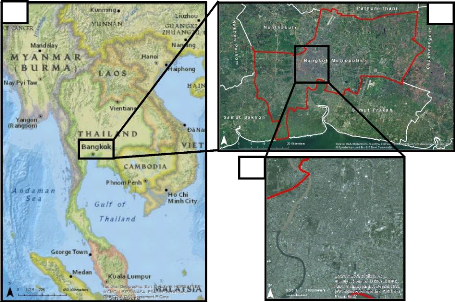
a.
c.
b.
Figure 5: Localization of the study area. a. Geographical
location of Bangkok in Southeast Asia, b. localization of the study
area
in Bangkok, c. study area
III.1.1. General context
Since the 1960th, Bangkok has known an astonishing
physical growth from 6 km2 to the current city area. Its major
river, the Chao Phraya, has performed as the central artery of the whole city
and has significantly influenced settlement formation and configuration
(MATEO-BABIANO, 2012). The population of Bangkok was estimated to be around one
million people in 1950 while today it is close to 12 million (FRASER, 2002).
This number is continually increasing due to the excellent economic potential
of the city that attracts people from the countryside as well as expatriates
from all over the world. Furthermore, abundant tourists visit Bangkok every
year, adding people in this already overpopulated city (THAIUTSA et al.,
2008).
Bangkok presents the case of a dynamic city with competition
between its traditions and the Western contemporary influences on its urban
spaces. The city shows the same seemingly disorganized quality that
characterizes the Asian space and therefore the diversity of the street space
is alike the forest environment, where a cacophony of sounds, sights, smells,
tastes and touch can be experienced altogether (MATEO-BABIANO, 2012).
Regrettably, the other side of the coin of a megacity like
Bangkok is the multiple kinds of pollution that occur which include
atmospheric, auditory and visual. Water pollution is also critical on the fact
that the canals are like open sewer, the groundwater is therefore in really bad
shape. The publications over this subject are countless and won't be developed
through this work.
III.1.2. Climate and Altitude
Bangkok has a seasonal monsoonal climate. According to the
Köppen classification it is an Aw climate type (KHEDARI et al., 2002). The
daily average temperature stays relatively constant over the year with a mean
annual temperature of 28.1°C. The monsoonal rainy season stands from July
to October while the dry season extends from November to June with the three
first months (until February) cooler, making it be called the «cool»
season. The last month of the dry season (from March until June) shows high
solar intensity as well as high heat and longer days and is therefore called
the hot season (Figure 6). The heat in this season is even more felt by the
effect of pavement and buildings (THAIUTSA et al., 2008).
|
RAINFALL (MM)
|
400 350 300 250 200 150 100 50
0
|
|
31 30 29 28 27 26 25 24 23
|
TEMPERATURE (°C)
|
Jan Feb Mar Apr May Jun Jul Aug Sep Oct Nov Dec
Total rainfall (mm) Average Temperature (°C)
Figure 6: Bangkok Climate Chart3
15
3 Data from
http://fr.climate-data.org/location/6313/
visited on 18/03/2014
16
Climate change is a significant threat that will create,
through the rising of the sea level, profound impacts on the Chao Phraya Delta
(ROUND, 2008). As Bangkok is situated only 2 m above de sea level with some
important parts of the city that are only at 0.5 m or less, clearly much of the
inner city could be flooded by the turn of the century (JARUPONGSAKUL,
20004; cited in ROUND, 2008). Over 14% of the city's total area is
seasonally flooded during the wet season (THAIUTSA et al., 2008).
III.1.3. Land use
THAIUTSA et al. (2008) calculated the areas of the main land
uses in Bangkok from GIS analysis of satellite imagery. As no more literature
was found about the land use in Bangkok, the following information stems from
this article.
Bangkok includes a quite large amount of unconstructed areas
within its boundaries. As shown in Table 2, just over 50% of the metropolis is
made of building, roads and other constructed surfaces, followed by an
unexpected 26% of land used for food production, mainly farmland and shrimp
farms on the periphery of the city boundaries. Finally, only 4.2 % of the
city's total area is green space, if one excludes agricultural land. The green
spaces are mostly made of trees found in the streets and naturalized areas with
1.2% of developed green spaces. The developed green spaces are nearly equally
split between actual parks accessible to the entire population, sports field
and golf courses which are not readily accessible to all the citizens of
Bangkok.
Table 2: Area of main land uses in Bangkok (variables
source: THAIUTSA et al., 2008)
|
Land use
|
Km2
|
Percent
|
|
Parks, sports field, and golf courses
|
19
|
1.2
|
|
Trees
|
47
|
3.0
|
|
Water, seasonally flooded
|
225
|
14.3
|
|
Agriculture/fish farms
|
411
|
26.2
|
|
Developed
|
792
|
50.5
|
|
Other, not used
|
75
|
4.8
|
|
Total
|
1569
|
100.0
|
The land use is very different in the central part of the city
in comparison with its eastern and western edges that are adjoined with food
producing areas and forest covered provinces. Thus, those districts have the
highest rate of tree and food producing areas within Bangkok. On the other
hand, the districts situated in the center of the city, have the highest
population density with 14,000 persons per km2 and 8000 persons per
km2 respectively, these amounts being 2 to 4 times higher
4 JARUPONGSAKUL T., 2000. Potential impacts of sea-level rise
and the coastal zone management in the upper gulf of Thailand. pp. 138-151 in
SINSAKUL S., CHAIMANEE N. and TIYAPAIRACH S. (eds.), Proceedingsof the
Thai-Japanese geological meeting: The comprehensive assessment on impacts of
sea-level rise. Geological Survey Division, Department of Mineral
Resources, Bangkok.
17
than in the other districts groups. This is of greater
importance as the study will focus on the green patches of this part of the
city. Those variations in population density distort the per capita green space
values. Hence, the per capita green space averages 2.8 m2 in those
two districts while it rises to a mean of 11.8 m2 for the entire
city. About 40% of those green spaces are actually park spaces (the rest being
tree cover) which represent around 1.2 m2 per inhabitant. The BMA
tends to increase the park space per capita so it will reach 2.5 m2
in 2023 with an ultimate goal of 4 m2 per person.
18
IV. METHODOLOGY
As a reminder, the goal of this study is to investigate the
ornithological characteristics, together with the environmental factors
affecting them, within various vegetation patches in Bangkok in order to
implement the basis for a long term monitoring.
In order to reach the fixed goal, a suite of processes was
followed. First, the vegetation patches were sampled within the study area. A
field phase was then realized within those green patches to collect the raw
ornithological data. On the other hand, the environmental data were obtained
from a digitalization out of satellite imagery using the GIS software ArcGIS(c)
10.1. Various variables were then calculated to permit the description of the
urban green patches' ornithological and environmental characteristics.
Different statistical methods (principally multivariate) were finally used in
order to point out the bird communities formed and how the environmental
features affect them.
VEGETATION PATCHES SAMPLING
The three main components of a landscape structure are (FORMAN
and GODRON, 1986):
- The patches: functional units of the landscape which
represent homogeneous environmental conditions and whose boundaries are
distinguished by discontinuities in the state variable of a significant
magnitude for the ecological process or the considered organism. All patches
showing similar characteristics for the considered process is called
«type» or «class».
- The corridors: units of a characteristic linear form.
The «corridors» perform the ecological function of passage, filter or
barrier. They are often present in a network-like landscape.
- The matrix: across types, the «matrix» is
the most common and the less fragmented. This type can also be considered as
the background of the landscape within which are situated the other
elements.
This work will focus on the birds of the «urban
green» patch type, the matrix in this case being the concrete of the urban
zone. Unfortunately, the avian distribution in the corridors won't be
approached because of the lack of time, although it can hold a high level of
bird diversity (SODHI et al., 1999; WHITE et al., 2005).
The precise localization of the green spaces in the study area
was a first necessary component for the proper achievement of the sampling.
Like many cities, Bangkok has spatially explicit planning, land use, and land
cover maps for the entire city. Regrettably, it was not possible to get those
maps, especially in the context of the political crisis that occurred during
the time of the field work.
19
A digitalization of those green patches was made possible
thanks to the interpretation given out of Google Earth(c) satellite imagery
(version 7.1.2.2041, accessed on February 2014), Google Maps(c) and various
recent tourist maps of the city. A preliminary process of exploration was
achieved ten days before the start of the survey to validate in the field the
potential green areas.
Some factors affected the selection of the parks and restricted
the sampling possibilities:
- the time of the field work was short (3-4 months)
- we focused on green areas localized in the most densely
urbanized area of the city - all the green patches of Bangkok were not open to
public
- all the green patches were not accessible considering their
spatial situation
Finally, we selected 25 green patches on a total sampling
basis, which means that all the green areas identified accessible and public
allowed were designated for the study. Most of them were urban public parks,
with two crossroad greeneries, one temple, one University's park, and adding to
that, a cemetery (Appendix 1). As we realized the study in all public areas, we
assumed the anthropic effect as equal. Furthermore, as poacher's activities are
unobserved and because people don't really hunt birds in the city (ROUND,
2008), the presence of people will not reduce the bird presence but is more
likely to affect our chances to detect them.
Ideally, the order of visit of the different parks should be
determined on a random basis. However, practically, in order to optimize the
movements across the study area, small green patches, close to each other were
all visited within a same survey period. Because some species have a more
active acoustic activity in the early morning, the order of visit into the
parks surveyed together was inversed every day. Thus, a green patch visited in
the early morning one day, was visited at the end of the morning the next day
in order to increase the probability of encountering all the present species.
The same scheme was followed for the afternoon.
20
Figure 7 below illustrates the patches' location within the study
area.
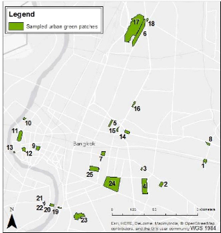
Figure 7: Map of the patches sampled in Central Bangkok
RAW DATA COLLECTION
IV.2.1. Ornithological surveys
Counting the avian fauna can get quite complex and a review of
the literature provides plenty of methods that were employed to do it (POMEROY,
1992). According to JONES (1998), «It is better to get reliable data
using a simple method than unreliable data from a complex one, even if the
latter (potentially at least) could provide more information». The
major reason for adopting a simpler method is to make it easily repeatable,
i.e. it allows the study to be significant even if the operators are different,
don't have the same level of training or don't put the same amount of effort in
the study (JONES, 1998). It is all the more important for this study as it
implements the basis for a long term monitoring and others will repeat this
work in the future.
21
The two basics aspects of counting birds are the number of
species and the number of individuals (POMEROY, 1992). We will record both
while making counts, but they are not necessarily related. Indeed, the
importance of birds in the ecosystem varies from place to place because
different places have variable numbers of species and individuals (POMEROY,
1992).
The counting method depends upon many things, such as why the
counting is made, which level of accuracy needs to be achieved, which resource
is available and what time of the day and of the year the survey is done
(POMEROY, 1992). Moreover, many factors affect bird activity and behavior,
which influences the chances of recording them. Among the more important
factors are the season, the time of the day and weather condition (JONES,
1998).
- Season
Seasonal effects on birds can be difficult to cope with. JONES
(1998) shows the case of a species which is breeding: while the males may be
singing and calling to defend their territory, which makes it easy to record
them, the females that are nesting won't be seen.
The ornithologist survey we realized within the field phase
took place between February 17th and June 4th 2014 i.e.
during Thailand's hot season. As it was spread over a short period of time, the
seasonal effect was minimized. However, as the migration period occurred in
April-May, and the non-breeding visitors leave Bangkok around this time as
well, the bird's seasonal status (ROUND, 2008) were recorded on the bird
species list created.
The ten days before the start of the survey, spent venturing
in Bangkok urban green spaces, were also essential in order to get familiar
with the bird species and to design the practical details of the bird survey.
Moreover, we revisited the sixth first patches at the end of the field work
period so the bird species knowledge can be assumed as equal in all the
patches.
- Time of the day
As the aim of a census is to record as many as possible of the
birds that are present, as quickly as possible, and as most of the birds show
trends of morning and late evening peaks of activity (JONES, 1998), we chose
those times for our surveys. Consequently, to follow the common study design
pointed out by JONES (1998), the data collection began 30 minutes after dawn
(6.30 am) in order to avoid the saturated acoustic atmosphere, well known as
the dawn chorus, when the louder birds would be over recorded at the expense of
the quieter ones. The survey ended during the mid-morning when bird activity
declines (9.00 or earlier depending on the length of the path). The second
survey period occurred before dusk, at about 4.00 pm until 6.30 pm.
22
- Weather condition
We avoided adverse weather conditions like rain in order to
delete the bias it could lead to in the surveys. Indeed, the bird activity is
generally highly affected by those conditions, as well as the observer's
capacity to see or hear them (JONES, 1998). Therefore, surveys were sometimes
postponed until the following day due to the weather while approaching the
rainy season.
We calculated species richness and abundance from the data
gathered from six repeated passages into the patches, 3 in the morning and 3 in
the afternoon to optimize the detections and the number of events in order to
increase the analytical precision. Such surveys offer baseline conservation
data regarding the distribution of the species, the richness of the sites or
habitats and allow comparisons to be made between areas (JONES, 1998).
The principle was to walk along the patches tracks at a mean
pace of 25 meters per minute and to record and count all the birds seen or
heard. Adding to the binoculars (Nikula (c) V061042) and a field guide of the
birds of Thailand (ROBSON, 2002), we also used a GPS receiver (Garmin GPSMAP
62) to survey the length of the path followed and afterwards to deduct the time
spent surveying.
We used this survey technique, at the expense of other
widespread practices, after some tests in the field which demonstrated the best
results of the latter. For this reason, we didn't proceed with the «point
counts» technique even though it is the most common method used to study
the link between birds and habitat (BIBBY et al., 1998b). Indeed, as the
patches were only sampled during three consecutive days, there wasn't
sufficient data collected for most species to use this technique (except for
Rock Pigeon or Eurasian Tree Sparrow or other very common urban species). We
chose not to apply the «distance» technique neither because it needed
too much prerequisites.
While «simply» recording and counting all the birds
seen or heard along the linear survey as described above, we observed for each
species a relative abundance and not an absolute abundance. It is not suitable
to compare on this basis the abundance of two species because one could be
easier to detect than the other. Similarly, one species' abundances can't be
compared between surveys made in two different environments. However, in this
case, the different surveys were done in similar contexts - urban green spaces
- and the hypothesis can be done that the detection probability of a same
species is similar within all the patches (BIBBY and BUCKLAND, 1987; JONES,
1998).
It is important to note that we counted separately the birds only
flying over the surveying zone.
IV.2.2. Environmental surveys
23
Each of the 25 patches surveyed was characterized by different
land covers. For reason of time availability and lack of permit from the
Bangkok administration, local ecological variables like the tree cover or
canopy height could not be surveyed directly within the urban green spaces
visited during the field work.
Nevertheless, in order to get environmental variables for the
purpose of data analysis, land cover features within the 25 green patches were
digitalized from a ESRI basemap (world satellite imagery5) using the
GIS software ArcGIS(c) 10.1 (Figure 8).
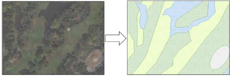
Figure 8: Digitalization of the land cover
5 Sources: Esri, DigitalGlobe, Earthstar Geographics,
CNES/Airbus DS, GeoEye, i-cubed, USDA FSA, USGS, AEX, Getmapping, Aerogrid,
IGN, IGP, swisstopo, and the GIS User Community
24
The land covers were categorized into five types described in
Table 3.
Table 3: land cover type description
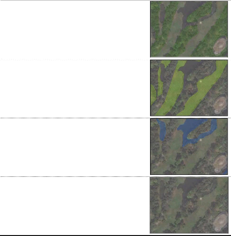
Woody vegetation Tree canopy
Herbaceous Grassy area, planted flowers and bushes
vegetation
Water River, water bodies and ponds
Buildings, path and other constructed surfaces
Concrete within the green patch
Land cover type Description Digitalization
25
DEFINITION AND CALCULATION OF THE VARIABLES IV.3.1.
Ornithological variables
The number of species recorded in each patch was based on the
total number of species that were observed on a track across the 6 sampling
periods.
Moreover, the amount of bird individuals per species seen or
heard around the track were also recorded. As double counting or omissions can
occur while recording birds with this method, the abundance collected could not
be assumed as real. Therefore, the field hours were recorded in conjunction
with the number of individuals of each species observed. This allowed a
relative frequency of abundance to be calculated for each species by dividing
the number of birds recorded by the time spent on the field, giving a figure of
birds per hour for each species (ROBERTSON and LILEY, 1998). We can therefore
assume that there is an actual relationship between the observed frequencies
and the bird densities into the patches. However, the abundance data obtained
do not give precise indications of density but if the hypothesis is made that a
species is as easy to detect at one site as another, then encounter rates can
be compared for a species between sites by being split into crude ordinal
categories of abundance (Table 4). The categories allowed abundance scores to
be given and future surveys to detect large scale changes in the abundance of
individual species (ROBERTSON and LILEY, 1998).
Table 4: Crude ordinal scale of abundance deducted from the
encounter rate data (adapted from ROBERTSON and LILEY, 1998)
Abundance category
(Number of individuals per hour) Abundance score
Ordinal scale
0 0 Not recorded
0-0.1 (not included) 1 Uncommon
0.1-2.0 2 Frequent
2.1-10.0 3 Common
10.1-40.0 4 Abundant
>40.0 5 Very Abundant
For the subsequent analyses, some birds encountered during the
field survey were not counted. This applied for passage migrants only seen
punctually in some patches as well as non-breeding visitors recorded during the
first months of the survey that were gone at the end and also for presumed
escaped captives birds. Similarly, the birds recorded as flying over the census
area were not used in the analyses (principally Swifts, Asian Openbills or Barn
Swallows).
26
IV.3.2. Environmental variables
Six environmental variables emerged from the previous
digitalization (Table 5).
Table 5: Parameters defining the patches
Patch Parameter Unit
Area m2
Perimeter m
Wooded Vegetation Surface m2
Herbaceous Vegetation Surface m2
Water Surface m2
Concrete Surface m2
Central point (x, y) -
? Biogeographic variables
The Island Biogeography Theory (IBT; MACARTHUR and WILSON,
1963; 1967) predicts how the area and isolation of oceanic islands affect their
species richness through the variation of extinction and colonization rates.
The IBT was later revisited to any «area where the species can exist,
surrounded by an area in which the species can survive poorly or not at all and
which consequently represents a distributional barrier» (DIAMOND,
1975). In our study, the green patches can be considered as `islands' of
habitat in the inhospitable matrix of the concrete of Bangkok.
From the patches areas (AREA) of the 25 green spaces, we were
able to calculate an isolation variable, the weighted connectivity (WCON)
between the patches in order to combine one fragment area with the proximity of
the other 24 fragments (BICKFORD et al., 2010). The weighted connectivity of
focal fragment ?? was calculated as
25
?
(???? )/?????? ???? ??=1,?????
where ???? is the area of fragment ??, ???? is the total area
of all fragments and ?????? is the shortest distance between fragments ?? and
??.
? Landscape variables
The patch parameters allowed us to calculate four indices
commonly used to characterize the landscape (BICKFORD et al., 2010; BASTIN and
THOMAS, 1999; BUREL et al., 1999) presented in Table 6.
27
Table 6: Landscape indices
Indices Code Unit
Shape Index SFACTOR -
Landscape Richness Index nLC -
Patch Equitability Index
? Wooded Vegetation WOOD %
? Herbaceous Vegetation HERB %
? Water WATER %
? Concrete CONC %
Shannon Heterogeneity Index SHANL -
The Shape Index (SFACTOR) is calculated as (BICKFORD et al.,
2010)
??
2v??* ??
where ?? is the measured perimter of the patch divided by the
circumference of a perfect circle of
the same area (2v?? * ??). So, a long and narrow patch will
have a higher Shape Index than a more nearly circular patch. It is important in
the context of the current work because the patch shape can affect its
ecosystem vulnerability to external influences. As a reminder, a circular form
offers the greatest possible area for a given perimeter.
The landscape data recorded in each patch allowed the
quantification of the landscape composition that can be expressed by 3 types of
indices (BUREL et al., 1999). The first one concerns the landscape richness and
is expressed by the number of land cover classes it contains (nLC). The second
index type refers to the equitability of the land cover classes it outlines,
i.e. the proportion taken by the different land covers described earlier (WOOD,
HERB, WATER, CONC). The third type of index of landscape composition is the
heterogeneity, which combines the two previous ones. Heterogeneity is synonym
of diversity and many indices allow its quantification. The one used in this
work is the Shannon Index applied to the landscape (SHANL), defined as
(SHANNON, 1948; SPELLERBERG and FEDOR, 2003)
- ? ???? ???? ???? ??=1
where ???? = ???? / ?? is the relative frequency of each land
cover within each patch. It gives an index of the combination of richness and
evenness of the land cover.
28
? Spatial variables
Several spatial variables were considered in order to test if
some of the previous landscape variables could be correlated with the patch
position into the study area. Those spatial variables could as well explain the
distribution of some species. They were defined on the basis of the WGS84
geographic coordinates of the central point of each park. In addition to the
simple latitudes (X) and longitudes (Y) other spatial variables were
calculated: X2, Y2, XY, X2Y, XY2,
X2+Y2, X3, Y3,
X3+Y3 (GAILLY, 2013).
? Correlations matrix of the environmental variables
A correlation matrix was realized in order to identify the
highly redundant variables within the landscape and spatial variables. The goal
hereby is to delete the correlated variables and therefore to decrease the
number of variables in order to allow a better visibility of the results. The
correlation coefficient of Pearson has to be higher than 70% in order to
present a correlation.
DATA ANALYSIS
The data analysis was split into four sections in order to
achieve the four objectives of the thesis. We started with an evaluation of the
bird diversity through the calculation of various parameters of the species
assemblages in each patch. Following that, we analyzed the ornithological
communities potentially found in the overall patches through multivariate
analysis. The environment within the patches was then characterized and
finally, the response of the bird assemblages to the driving forces affecting
their habitat in Bangkok was investigated. Descriptive analysis and map of the
distribution of those parameters across the study area were performed in order
to illustrate the results before further interpretation.
IV.4.1. Ornithological distribution analyses
The two first descriptive parameters of the bird distribution
considered are species richness and abundance. In order to get closer with a
major urban issue presented before, namely the biotic homogenization
phenomenon, a Community Specialization Index (CSI) was calculated.
? Species Richness
Species Richness is one of the basic measures of diversity.
The species richness of a patch was defined in this work as being the total
number of species recorded across the 6 sampling periods.
In order to allow a comparison between the assemblages, the
sampling effort is assumed to be equal. However, the completeness of the
surveys in the 25 patches must be considered. This calculation required the
drafting of species saturation curves. Thus, for each patch, the random
29
settlement of the samples allowed the establishment of a mean
cumulative richness curve. The most accurate the survey, the more this curve
tends to an asymptote. The sample completeness is calculated as the ratio
between the number of species observed and the real number of species within a
patch. The EstimateS(c) 9.1.0 software was used to compute non-parametric,
asymptotic species richness estimators for incidence-based data (COLWELL, 2013)
and allowed the establishment of those mean curves of cumulative richness. The
real number of species could be estimated via a first order Jack-knife
extrapolation (GAILLY, 2013) which is function of the number of species that
only appeared in one sample: «unique» species (HELTSHE and FORRESTER,
1983).
A map was created showing the species richness of each patch
within the study area in order to obtain an overview of the richness
distribution. Then, in order to show the species distribution in the overall
patches, we estimated for each species a distribution range going from very
low, while the species was only present in 1 to 5 patches to very high when the
species was recorded in 20 to 25 patches. A column chart was drawn in order to
illustrate the bird species distribution.
? Abundance distribution6
In order to get a bird abundance estimation within each patch,
we decided to use a heterogeneity index since a simple sum of the species
abundance scores for each patch doesn't take into account the individuals
repartition between the different species. Thus, to synthetize the number of
species and the equilibrium of the individuals' repartition into one quantified
variable, we used the Shannon Index of Species Diversity (SHANNON, 1948;
SPELLERBERG and FEDOR, 2003):
n
H = - I pt Inp??
1=1
where pi = ni/N is the proportion
of species i in the green patch. This index gives an appropriate
index of bird diversity at a site because it takes into
account the abundance of each species recorded at this site (SODHI et al.,
1999).
Then, to show the species abundance distribution along the
patches, we estimated for each species its total abundance on the study area
going from very low, while the species had a cumulative abundance score ranging
from 1 to 25, to very high when the species showed a cumulative abundance score
ranging from 101 to 125. A column chart was drawn as well in order to
illustrate the abundances distribution.
6 As a reminder, the abundance data was split into
ordinal categories of abundance which were given an abundance score ranging
from 1 to 5.
30
? Functional homogenization
«Biotic homogenization» is a quite contemporary term
traducing a biodiversity erosion process resulting from a diminution of the
species community variability among sites or habitats and not from an
impoverishment of the species communities in themselves (VAN TURNHOUT et al.,
2007; SAX and GAINES, 2003).
This homogenization process generally appears while there is
fragmentation or degradation of a habitat and is linked with an augmentation of
generalist species to the detriment of more specialized species. Hence, the
degree of specialization of a bird species to a given habitat class is
positively related to the species abundance along that habitat class gradient
(DEVICTOR et al., 2008). Therefore, a more specialized species will show higher
densities with the augmentation of a particular resource while more generalist
species will demonstrate little variation across habitats. The approach of
JULLIARD et al. (2006) was used in order to quantify the Species Specialization
Index (SSI) as the coefficient of variation (Standard Deviation / Average) of
the species densities among the patches (DEVICTOR et al., 2008). The SSI
allowed ranking all considered species from the most to the least specialized,
whatever the species size, ecology, habitat preference and under any site
classification (JULLIARD et al., 2006).
Then, a CSI was measured in order to estimate the functional
homogenization. The CSI for a green patch ?? is given by the mean SSI of
species present at a given site (DEVICTOR et al., 2008).
? ?????? × ????????
??
??=1
? ??????
??
??=1
???????? =
where ?? is the total number of species recorded, ?????? is
the relative abundance of species ?? in patch ??, and ???????? its
specialization index.
IV.4.2. Ornithological communities analysis
The research for species associations is one of the usual
problems of community ecology (LEGENDRE and LEGENDRE, 2012). Until now, the
analyses focused on the overall species diversity and did not take into account
species assemblages. In order to include them, we need to use multivariate
methods.
Those methods can be classified into two main groups:
- Ordinations methods: identify gradients within the
data set whilst opposing species and sites that are the most different (find
continuities).
- Cluster methods: identify sites or species groups
that share a maximum of similarities classification of the objects in groups
(find discontinuities).
Those two approaches, while opposed, are in fact complementary
to analyze multivariate data sets (DUFRÊNE, 2003). They will both be
outlined in this work (Figure 9) and they were performed using the RStudio(c)
software (Version 0.98.976). A research of indicator species into the different
clusters was then operated using the same software.
The adopted methodology was set using the abundance scores
matrix. Indeed, the abundance indices truly give more interpretation
possibilities than presence/absence data. We thus assume that the necessary
conditions (equal detectability), in order to compare the bird assemblages
between the patches based on the abundance scores, are respected (JONES,
1998).
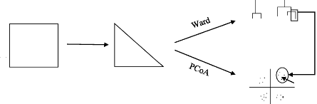
Patch n°
Bray-Curtis
DISTANCE MATRIX
DATA
MATRIX
CLUSTER
DENDROGRAM
IndVal
Bird Species
31
ORDINATION PLOT
Figure 9: Method used for the ornithological communities
analysis: Bray-Curtis = methods used for the creation of the
distance matrix, Ward= Ward's minimum variance method used for
the cluster analysis, PCoA= Principal Coordinate Analysis used
for the ordination analysis, IndVal=Indicator Species
Analysis.
? Creation of a distance matrix
Firstly, the data matrix was conversed into a distance matrix
through the estimation of the sites «proximity» regarding the
observed species and their abundance. It is therefore a multivariate measure of
the differences existing between sites.
32
Among the distance calculation methods, that of Bray-Curtis (D
14) was selected for the analysis on the species communities based on the
abundance data. Bray-Curtis index is a distance coefficient calculated from the
Steinaus similarity coefficient (S17) that compares two sites (x1, x2) in terms
of the minimum abundance of each species. The D14 formula is
2W
where W is the sum of the minimum abundances of the different
species, this minimum being defined as the abundance at the site where the
species is the rarest. A and B are the sums of the abundances of all species at
each of the two sites respectively (LEGENDRE and LEGENDRE, 2012). This index
was chosen because it can be used on abundances frequencies and because a same
difference between two sites for abundant of rare species has the same
contribution to the similarity.
? Cluster Analysis
The cluster analysis gives a graphical representation
(dendrogram) that was used to determine, from the Bray-Curtis distance matrix,
the similar bird communities' compositions among the different sites. It also
provided the opportunity to see how the sites rank in comparison to each
other.
A hierarchical agglomerative clustering method was used to
join together the more similar sites. The term «hierarchical»
signifies that the position of a site was definitively imposed within a branch
of the classification. The term «agglomerative» refers to the
discontinuous partition of the objects where those are considered as being
separate from one another. They are successively grouped into larger and larger
clusters until a single, all-inclusive cluster is found (LEGENDRE and LEGENDRE,
2012).
The Ward's minimum variance method was chosen (e.g. CONOLE and
KIRKPATRICK, 2011; GAILLY, 2013; LOUGBEGNON and CODJIA, 2011) because it aims
at finding compact, spherical clusters. To form clusters, this method minimizes
the variance across each group as the sites agglomeration progress in
minimizing the sum of squared deviation distances from the centroid of each
group. Compared to other clustering methods, the Ward's minimum variance method
overestimates the distances between sites while the first groups are shaped
(LEGENDRE and LEGENDRE, 2012).
The sites similarities calculated from the dendrogram and
named cophenetic similarities are different from the original similarities that
served to cluster the sites together. Hence, the calculation of the cophenetic
correlation allowed us to measure the relationship between the distances of
Ward's clustering and the original ones (LEGENDRE and LEGENDRE, 2012).
33
? Ordination analysis
The Principal Coordinate Analysis (PCoA) allowed us to
position the 25 patches, in a space of reduced dimensionality while preserving
their distance relationships calculated above as well as possible. The PCoA
used the distance matrix calculated before with the goal to find out the axes
that maximized that distance matrix (LEGENDRE and LEGENDRE, 2012).
Some distance measures might be negative and did not allow a
proper ordination of sites in a full Euclidean space. Therefore, they need a
correction for the negative eigenvalues before being used for ordination by
PCoA (LEGENDRE and LEGENDRE, 2012).
? Indicator species
An indicator species must meet two specific criteria
(DUFRÊNE, 2003): it must dominate into a group of sites (specificity
index, percentage of individuals in the group) and it must occupy all of the
sites within that group (fidelity index, percentage of occupied sites in the
group). The IndVal method (DUFRÊNE and LEGENDRE, 1997) was used to
identify the species that can be considered as associated to a site or a group
of sites. Hence, this method takes into account the specificity and fidelity
indices while calculating the species indicator value, giving a percentage
proportional to the previous indices. The highest IndVal value obtained
identifies the group where the species can be considered as indicator. In
addition, the IndVal method allows to test statistically if a species can be
considered as being indicator or not.
Moreover, the sum of the species indicator values can be
assumed as a criterion in order to compare the clusters formed and choose which
one explains the species distribution best (DUFRÊNE and LEGENDRE,
1997).
IV.4.3. Environmental characteristics
analyses
The following analyses aimed to achieve an investigation of
the environmental factors affecting the different patches. It is indeed
essential to examine those factors and their distribution within the study area
as a first step to interpret the ornithological distribution. We used a
multivariate approach using the RStudio(c) software (Version 0.98.976).
To determine the interactions that the environmental variables
tended to have with each other in our study area, we performed a principal
component analysis (PCA). The PCA is an ordination method that considers the
variables altogether and allows the creation of a space of reduced
dimensionality from an extraction of the axis that maximize the variance of
multidimensional cloud of points shaped by the initial environmental variables.
In other words, it condenses the dimension of the cloud of points and helps
choose a point of view to look at this cloud of points. The two axes are
perpendicular with each other (so they are not redundant) and each one
explains
34
a part of the initial cloud information. Those new descriptors
of the information are called principal component and are linear combinations
of the initial variables. The roles of those new axes are interpreted while
examining the initial variables that are the more correlated (ROBERTS,
2010).
Values of sites characteristics were correlated with the first
two principal axes using Pearson and Spearman rank-order correlations
coefficients. The reason we used the two methods is that Spearman's correlation
coefficient is a non-parametric method unlike Pearson's. Non-parametric methods
consist in finding a coefficient correlation, not between the values taken by
the two variables, but between ranks of those values. It allows to find out
monotone correlations although the variable distributions are skew. The Pearson
method only consists of finding the linear relation between values and is
easily biased if the two variables don't have a Gaussian distribution or show
exceptional values.
The comparison of the two correlation coefficients values
brought information about the bias of the correlation calculated. Hence, if
Pearson coefficient was higher than the Spearman's one, this means that
exceptional values could be present. This would increase the Pearson
coefficient value but not modify the more robust Spearman's coefficient
values.
IV.4.4. Environmental explicatory factors of the
ornithological distribution analysis
For the thesis to be more than descriptive work, an
investigation of the influence that the environmental factors have on the bird
distribution was realized. The analyses were divided in two sections. The first
analysis investigated the influence of the environmental factors on the
previously calculated descriptive parameters of the ornithological through
multivariate analysis (indirect gradient analysis). Then, Generalized Linear
Models (GLM) were realized to demonstrate the relations existing between the
environmental variables and our diversity measures. The third analysis directly
confronted the bird abundance data matrix with the environmental factors
through a multivariate analysis called the redundancy analysis (RDA; direct
gradient analysis).
? Indirect Gradient analysis
To determine how the ornithological descriptive parameters
(species richness, CSI and Shannon index) were affected by site
characteristics, the ornithological parameters were correlated with the
previous PCA axes using Pearson and Spearman correlation coefficients.
? Generalized linear models
Regressions equations allowed us to formalize the relationship
existing between explicative variables and variables to explicate. We used GLMs
in order to determine which variables or sets of variables had the largest
influence on the overall species richness, Shannon index of heterogeneity and
CSI.
35
For the following analyses, we transformed our previous set of
explanatory environmental variables so they approach a normal distribution. A
p-value was estimated for each variable through a Shapiro-Wilk test (ROYSTON,
1982) to confirm or not the normal distribution.
All GLM models were constructed in Rstudio(c). We used
information-theoretic methods to compare models incorporating different
environmental variables, because of the advantages of that method over stepwise
approaches for this type of analysis (WHITTINGHAM et al., 2006). To identify
the most biologically relevant models, we used the small sample size Akaike's
Information Criterion (AICc). We identified the model showing the lowest AICc
as the best model (BURNHAM and ANDERSON, 2004; WHITTINGHAM et al., 2006).
Two other criterions were important as well to give
information on the model quality. The residual standard error (RSE) that
describes the standard deviation of points formed around the linear function,
and estimates the accuracy of the dependent variable being measured. And the
coefficient of determination (Adjusted-R2) that describes the
percentage of the observation variability that is explain by the regression
equation.
? Direct Gradient Analysis
Relationships between communities and the overall
environmental variables were assessed with a canonical ordination method. The
RDA is a multivariate analysis method commonly used in ecology in order to
analyze simultaneously two data tables (e.g. GAILLY, 2013; SATTLER et al.,
2010). It is the multivariate analog of simple linear regressions. The RDA
analysis combines the ordination and regression concepts. It allows the
ordination of the «species» variables constraints by a canonical axis
that is maximally related to a linear combination of the environmental
variables (LEGENDRE and LEGENDRE, 2012). It allows the representation at the
same time of the species, the patches and the environmental variables in a
space of reduced dimensionality.
We used a RDA in this thesis to link the species abundance
data set together with the environmental variables. We also projected the Ward
clusters obtained previously in the space of reduced dimensionality in order to
characterize them.
36
V. RESULTS
ORNITHOLOGICAL DISTRIBUTION ANALYSIS
The 6 respective visits into the 25 patches allowed us to
survey 49 bird species. After deletion of the non-breeding visitors (9
species), passage migrants (2 species), presumed escaped birds (4 species) and
a resident bird species that was every times recorded as flying over the census
area (Hirundo Rustica), 34 species were kept for the analyses
(Appendix 2). The following results give an overview of the ornithological
descriptive parameters distribution in the 25 patches. The notations for the 3
variables will be as follow: bird_R (bird species richness), SHANB (Shannon
index of bird diversity), CSI (community specialization index).
A conservation value was first planned to be calculated for
each patch, however it has not been completed since out of all the bird
recorded, none of the species were listed as «threatened» or
«near threatened» in the «Asian Bird Red Data
Book» (BIRDLIFE INTERNATIONAL, 2001).
All of the 34 species can be assumed to be synanthropic
species in view of the situation of the study area. Two of the species kept for
the analyses were identified as invasive species according to the GLOBAL
INVASIVE SPESCIES DATABASE (2005): Columbia Livia (Rock Pigeon) as an
alien invasive species and Acridotheres tristis (Common Myna) as a
native invasive species. Nevertheless, the number of known alien species in
Thailand was still far from being realistically estimated (NAPOMPETH, 2002).
V.1.1. Species Richness
Table 7 shows the species richness distribution within the 25
patches and its completeness while comparing them with the Jack-Knife estimated
real richness.
Table 7: Observed and Estimated Real Richness within the
patches
Patch Observed
Number Richness
Punctual Richness
Estimated Real Richness Completeness
(%)
Jack-Knife Jack-Knife S.D. Average S.D. Min. Max.
37
1 18 19.7 1.05 91.5 14.3 1.75 11 16


2 19 22.3 1.67 85.1 14.0 0.89 13 15

3 19 21.5 1.12 88.4 14.0 1.79 11 16

4 25 26.7 1.67 93.7 20.5 2.43 17 24

5 23 25.5 1.12 90.2 17.3 1.97 15 19

6 26 26.8 0.83 96.9 22.2 1.60 20 24

7 16 16.8 0.83 95.1 12.7 1.86 10 15

8 18 21.3 1.67 84.4 11.2 1.47 10 14
9 17 17.8 0.83 95.3 12.5 2.66 9 16


10 18 19.7 1.05 91.5 14.2 1.60 11 15

11 15 15.8 0.83 94.8 11.5 2.26 8 14

12 19 22.3 2.11 85.1 13.2 1.72 11 16

13 12 14.5 1.12 82.8 7.2 0.98 6 8

14 17 17.0 0 100.0 14.0 1.41 12 16

15 15 17.5 1.71 85.7 8.8 2.48 6 13

16 15 15.0 0 100.0 12.0 2.10 9 15

17 31 33.5 1.71 92.5 26.5 1.22 25 28

18 12 13.7 1.67 87.8 7.2 1.17 6 9

19 16 17.7 1.05 90.5 9.5 1.64 7 11

20 15 16.7 1.05 90.0 8.7 2.66 6 12

21 10 10.8 0.83 92.3 5.8 1.83 4 9

22 9 10.7 1.05 84.3 4.8 1.72 3 7
23 21 24.3 1.67 86.3 15.5 1.22 14 17


24 24 24.8 0.83 96.7 20.5 1.87 18 23
25 20 21.7 1.67 92.3 13.8 1.17 12 15
All of the cumulative richness curves tend to an asymptote.
Figure 10 shows two distinct curves got for patch No. 8 and patch No. 3. Their
Jack-Knife estimated real richness tends to the same number of species (21.5
and 21.3 species respectively), however the two curves show different shapes.
Indeed, the surveys in patch No.3 reached faster the real species richness than
the surveys carried out in patch No. 8. Hence, at least four surveys were
necessary in this case to get reliable data. Concerning the slopes the curves
at the last survey, the No. 3 is 0.5 and No. 8 is 0.3. This signifies that in
theory to get one new species, 2 supplementary surveys needs to be realized for
patch No. 3 and 3 for patch No. 8. The samplings completeness is therefore
acceptable.
|
Species Richness
|
22 20 18 16 14 12 10
|
|
|
Patch No. 3 Patch No. 8
|
|
|
|
38
1 2 3 4 5 6
Number of surveys
Figure 10: Cumulative richness curves for the patches No.3
and No.8
Another observation made while comparing the species richness
results is the time of the day of the survey. After a verification of the
normality of the data, a paired t-test of Student was done in order to compare
the mean bird richness observed in a park during the morning to the one
observed in the afternoon. The test showed that the true difference in means
was not equal to 0 (p-value= 8.627x10⁻⁷). Thus, the average species
found during the morning surveys appear to be greater than the ones during the
afternoon surveys (see Appendix 3 for the entire results).
39
The Figure 11 below illustrates the previous richness
distribution within the study area.
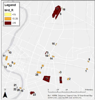
Figure 11: Map of the Species Richness per patch in the study
area (bird_R=Bird Species Richness)
Regarding the species distribution, 12 of the 34 species were
found in 21 to 25 of the patches surveyed while 11 of them were only found in 1
to 5 patches (Figure 12). Acridotheres grandis (White-vented Myna),
Acridotheres tristis (Common Myna) and Copsychus saularis
(Oriental Magpie Robin) had the higher range of distribution as they were
found in the 25 patches surveyed.
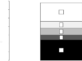
Number of species
35
30
25
20
15
10
5
0
12
11
4
4
3
40
Species Distribution
VERY HIGH HIGH MEDIUM LOW VERY LOW
Figure 12: Amount of species characterized by different
distribution (number of records) in the study area. Distribution classes: very
high (21 to 25 records), high (16 to 20 records), medium (11 to 15 records),
low (6 to 10 records) and very low (1 to 5 records)
41
V.1.2. Abundance Distribution
We generated a map (Figure 13) in order to compare the 25
patches Shannon index of diversity. We found that the patches No.21 and No.22
showed the lowest species diversity while the highest heterogeneity was
situated in the patches No.4, No.6 and No.17.
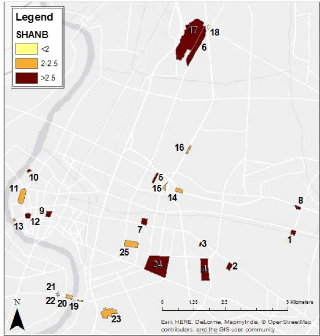
Figure 13: Map of the Shannon Index of Diversity per patch
in the study area (SHANB= Shannon index of bird
diversity)
30 25 20 15 10 5 0
Concerning the individuals' relative abundance, it is not
surprising that the two species that showed the highest count within the study
area appear to be two widespread urban species: Passer montanus
(Eurasian Tree Sparrow) and Columba livia (Rock Pigeon). On the
other hand, 16 species show a very low abundance (Figure 14).
35
5
42
6
5
2
Individuals Relative Abundance
VERY HIGH HIGH MEDIUM LOW VERY LOW
Figure 14: Amount of species individuals characterized by
different relative densities (total of the abundance scores) in the study area.
Relative abundance classes: very high (101 to 125), high (76 to 100), medium
(51 to 75), low (26 to 50) and very low (1 to 25 records)
43
V.1.3. Biotic homogenization index
The species having the highest SSI (species specialization
index) are Amaurornis phoenicurus (White-breasted Waterhen),
Passer flaveolus (Plain-backed Sparrow)7. Conversely,
Copsychus saularis (Oriental Magpie Robin), Acridotheres tristis
(Common Myna) and Acridotheres grandis (White-breasted Myna)
seems to be the more generalist species.
Concerning the CSI (community specialization index) calculated
for all the patches, Figure 15 illustrates its distribution within the study
area. The highest CSI was found in patch No.17 while the smallest was in patch
No.22.
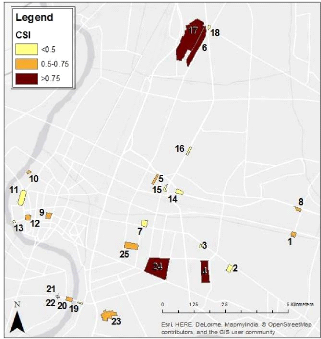
Figure 15: Community specialization Index
(CSI) distribution in the study area
7 Apus affinis (House swift) was also
listed a one of the most specialized species because it has been recorded only
once perched in a patch while it was seen often flying over the patches. This
species won't be taken into account in further statistical analyses.
44
In order to bring to a discussion of the previous parameters
describing the ornithological data, it will be interesting to compare the
evolution of their values in the 25 patches. Therefore, we decided to draw a
graph of their evolution on Figure 16. The x-axis of the graph organizes the
patches from the highest to the smallest bird species richness observed. We can
see that the general decreasing trend is similarly for the three indices with
the presence of peaks and troughs more contrasted for the Shannon index.
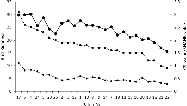
Figure 16: Comparison of the describing parameters of the
ornithological data calculated in the 25 patches studied
(bird_R
=bird species richness, CSI = community
specialization index, SHANB= Shannon index of species
diversity)
ORNITHOLOGICAL COMMUNITIES ANALYSIS
Data matrix for the analysis consisted of 25 sites x 33 bird
species.
V.2.1. Structure of the Ornithological data
The Ward's minimum variance method allowed us to classify the
sites in different groups on the basis of their species composition. The result
of the cluster analysis for the abundance data is illustrated on the dendrogram
on Figure 17 below.
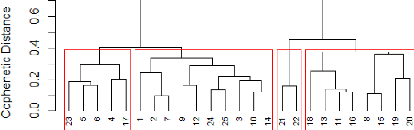
45
2 1 4 3
Figure 17: Dendrogram formed out of the Ward's minimum
variance method from the ornithological abundance dataset.
Four major groups
were identified
The cophenetic correlation coefficient calculated for Figure 17
has a value of 0.523.
A clear differentiation was firstly made between group 1-2 and
3-4, showing us the fundamental species abundances distance between the patches
of those groups. While comparing those results with the previous SHANB curve
(Figure 16: Comparison of the describing parameters of the
ornithological data calculated in the 25 patches
studied
(bird_R =bird species richness, CSI
= community specialization index, SHANB= Figure 16),
we can easily assume that the two first groups contain high species abundances
while the groups 3 and 4 show lower abundances. Still, four groups were chosen
in order to get more precise indication of the bird abundances distributions.
This being said, group 4 separates then 2 patches (21 and 22) showing together
similar low abundance trends. On the other side, the cut off between groups 1
and 2 is harder to describe.
46
The ordination method (PCoA in this case) offered the
possibility to illustrate the result of the cluster method in a space of
reduced dimensionality where the sites have been localized regarding their
species abundance scores (Figure 18).
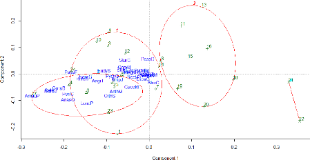
Figure 18: Factorial design created with the two first
axis of the PCoA concerning the abundance data. The red ellipses allow the
visualization of the four groups of sites defined earlier by the Ward's
method.
The two first axes of the PCoA explain 37.09% of the point
variability. The first axis (component 1) explains 24.03 % while the second
(component 2) explains 13.05%.The first axis shows well the isolation of groups
3 and 4 from the other groups that are partially overlapping each other.
Regarding the avian influence, it is quite hard to visualize bird assemblages
at this point.
V.2.2. Indicator Species
The IndVal method applied on the abundance data allowed the
identification of 11 significant indicator species (p-value < 0.05)
separating from each other two groups of sites. All the species listed in Table
8 were selected because they were indicators of the first and second group of
sites defined by the Ward clusters (None of the species listed in the two other
groups had a significant IndVal value). Some species were not significantly
kept from the IndVal analysis due to their lack of specificity or their rarity
in the surveys that didn't satisfy the two criterions of the method (i.e.
specificity and fidelity).
47
Table 8: Species selected via the IndVal method as being
significantly associated to a group of sites

Total sum of
Species Code Group IndVal p-value Frequency Abundance
score
RhipJ 1 0.437 0.006 18 45
CorvM 1 0.405 0.021 19 59
MegaH 1 0.376 0.001 23 76
SturN 1 0.374 0.007 22 56
NectJ 1 0.338 0.049 23 58
|
PycnB
|
1
|
0.310
|
0.014
|
24
|
81
|
|
LoncP
|
2
|
0.875
|
0.001
|
6
|
18
|
Pied Fantail
Corvus macrorhynchos
Large-billed Crow Megalaima haemacephala
Coppersmith Barbet Sturnus nigrocollis
Black-collared Starling Nectarinia jugularis
Olive-backed Sunbird Pycnonotus blanfordi
AnthM 2 0.692 0.031 5 10
OrthS 2 0.662 0.001 10 23
Yellow-Vented Bulbul
Streptopelia tranquebarica StreT 2 0.521 0.046 6
13
Red Collared Dove
Brown-Throated Sunbird Orthotomus sutorius
Common Tailorbird Pycnonotus goiavier
PycnG 2 0.588 0.002 11 23
Rhipidura javanica
Streak-eared Bulbul
Lonchura punctulata
Scaly-breasted Munia
Anthreptes malacensis
The two groups obtained in the previous table showed various
visible differences. First, considering the species record frequencies in the
25 patches, the first group holds widespread synanthropic species while
compared with the second one. However, the species of the second group show
higher IndVal indices than in the first one.
ENVIRONMENTAL CHARACTERISTICS
V.3.1. Correlations matrix of the environmental
variables
The correlation matrix (see Appendix 5) showed that a few of
the environmental variables (SHANL and nLC; SHANL and WOOD) presented together
a correlation coefficient higher than 70% and there was no correlation of the
landscape variables with the spatial variables. The landscape richness (nLC)
was eliminated from the landscape variables because the information given was
poor, while we decided to keep all the others.
By contrast, the spatial variables were for the most part
correlated. As their redundancy didn't offer real facilities for the subsequent
interpretations, 9 of the 11 variables were deleted. The two left are
X3+Y3 and Y3, as together, they were
correlated with all of the other spatial variables.
48
V.3.2. Principal Component Analysis of the
environmental variables
The PCA (principal component analysis) reported the
relationships between variables in the research of explanatory factors (for the
numerical values see Appendix 6). Before the start of the analysis, the
environmental factors have been log or squared-root transformed in order to
tend as much as possible to a normal distribution. Hence, the variables AREA,
HERB and WATE have been log-transformed while the WCON, SFACTOR, WOOD and Y3
were square root-transformed.
The two first axes of the PCA (PC1 and P) explain respectively
41% and 19% of the total variance of the data set, which means a total of
60%.
As we assume an axis is correlated if |r|>0.60 (Table 9),
the axis 1 of the PCA appears positively correlated to SHANL (91%), logAREA
(76%), logHERB (74%), SqrtSFACTOR (73%) and logWATE (68%) and negatively
correlated to SqrtWOOD (80%) regarding the Pearson correlation coefficients
(Figure 19). Concerning their Spearman correlation indices, they are quite
close of the previous ones except for the SqrtFACTOR variable that doesn't
appear correlated in this case (Figure 19). It is also remarkable that the
variable WCON shows here an opposite sign. This is due to the presence of three
exceptionally great values that overestimate the Pearson correlation
coefficient value.
The landscape heterogeneity appears to parallel the all other
factors on the first axis except for the percentage of wooded area and the
connectivity of a site (the latter correlation is low). This axis opposes
therefore the more open, large sites having a more heterogeneous landscape to
the more wooded ones. It is true that within our study area, a bunch of very
small patches were wood highly covered while the large patches contained more
water and herbaceous cover, meaning more heterogeneous landscapes.
Axis 2 seems to be relatively correlated with the spatial
variables (Y3: r =65%) regarding its Pearson coefficient, especially with the
longitude which is a direction going from the South to the North. However, the
Spearman correlation coefficient is lower than 0.6 because of three exceptional
values (three patches being together far more North than the others). Moreover,
the percentage of concrete in the sites seems to be negatively correlated to
this axis (CONC: r =-66%).
Then, Figure 20 displays the representation of the patches
along the two axes with the roles of those new axes interpreted.
49
Table 9: Pearson and Spearman correlation coefficients
between the environmental variables and the two axes of the PCA.
The numbers
highlighted show a correlation with the axis
|
Environmental
Factors
|
|
PC1
|
|
P
|
|
PEARSON
|
SPEARMAN
|
PEARSON
|
SPEARMAN
|
|
logAREA
|
0.761
|
0.676
|
0.081
|
-0.020
|
|
SqrtWCON
|
0.305
|
-0.274
|
0.588
|
0.353
|
|
SqrtSFACTOR
|
0.731
|
0.569
|
0.252
|
0.061
|
|
SqrtWOOD
|
-0.810
|
-0.786
|
0.386
|
0.475
|
|
logHERB
|
0.735
|
0.705
|
-0.341
|
-0.374
|
|
logWATE
|
0.683
|
0.731
|
0.208
|
0.249
|
|
CONC
|
0.310
|
0.200
|
-0.657
|
-0.690
|
|
SHANL
|
0.914
|
0.921
|
-0.302
|
-0.202
|
|
SqrtY3
|
0.394
|
0.245
|
0.650
|
0.403
|
|
X3Y3
|
0.456
|
0.409
|
0.482
|
0.563
|
PEARSON SPEARMAN
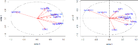
Figure 19: Representation of the environmental variables in
the Pearson and Spearman correlation circles formed by the two
first axes of the PCA
The longer the red arrow is, the more variance is explained
from the factorial design and the closer the arrow is from an axis, the more it
contributes.
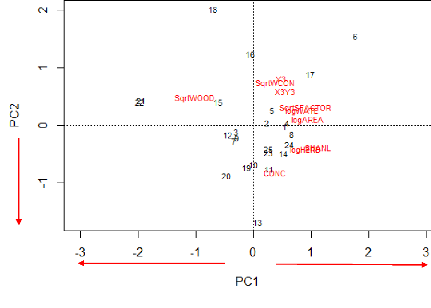
More wooded
-More open
-Larger areas
-More heterogeneous
With more concrete
50
Figure 20: Factorial design created with the two first axis
of the PCA concerning the environmental data.
51
ENVIRONMENTAL FACTORS EXPLAINING THE ORNITHOLOGICAL
DISTRIBUTION V.4.1. Indirect gradient analysis
The study of the role played by the environmental factor on
the ornithological distribution started with an analysis of the correlation of
the ornithological descriptive parameters with the two axes of the previous PCA
on the environmental factors.
PEARSON SPEARMAN
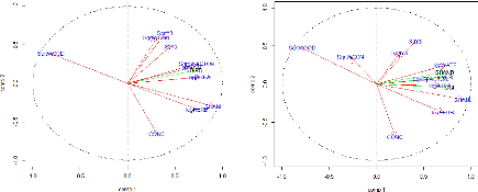
Figure 21 Representation of the environmental variables
(red arrows) together with the ornithological descriptive parameters (green
arrows) in the Pearson and Spearman correlation circles formed by the two first
axes of the PCA. Only one green arrow represented the three ornithological
parameters in the Pearson correlation circle for a better visibility as the
three arrows were merged together.
Figure 21 and Table 10 show both the positive correlation of
the ornithological description variables with the first axis of the PCA. This
means that species richness, Shannon index and CSI, became greater within
patches showing larger areas as well as more open and heterogeneous
landscapes.
Table 10: Pearson and Spearman correlation coefficients
between the ornithological variables and the two axis of the PCA.
The
numbers highlighted show a correlation with the specified axis.
|
Ornithological Factors
|
PC1 P
|
|
PEARSON SPEARMAN PEARSON SPEARMAN
|
|
bird_R
|
0.783
|
0.725
|
0.150
|
0.089
|
|
SHANB
|
0.724
|
0.724
|
0.156
|
0.156
|
|
CSI
|
0.730
|
0.772
|
0.171
|
-0.038
|
52
V.4.2. Generalized linear models
For the following analysis, it is important to note that three
environmental variables didn't reach a normal distribution (Shapiro-Wilk test:
p<0.05): WCON, SHANL and Y3. We kept the same transformation as before for
the other environmental variables. Table 11 presents a summary of the GLMs.
Table 11: General linear models and summary statistics for
ornithological variables. Predictor environmental variables are patch area
(logAREA, log-transformed), weighted connectivity (SqrtWCON, Square
root-transformed), S-Factor (SqrtSFACTOR, Square root-transformed), Wood cover
(SqrtWOOD, Square root-transformed), Herbaceous cover (logHERB,
log-transformed), Water cover (logWATE, log-transformed), Concrete cover
(CONC), Y3 (SqrtY3, Squared root transformed),
X3+Y3(X3Y3). a= first parameter, b= second parameter
(environmental factor coefficient), R2= coefficient of
determination, RSE= Residual Standard Error, AICc = Akaike's information
criterion corrected for small sample size. The best models are indicated in
bold for each ornithological variable.
Coefficients
Model R2 RSE AICc
a b
|
~logAREA
|
-13.612
|
2.993
|
0.721
|
2.692
|
125.524
|
|
~SHANL
|
8.531
|
10.176
|
0.467
|
3.720
|
141.691
|
|
~logWATE
|
13.536
|
2.866
|
0.428
|
3.855
|
143.475
|
|
~SqrtSFACTOR
|
-8.423
|
22.996
|
0.323
|
4.191
|
147.656
|
|
~logHERB
|
13.484
|
2.126
|
0.236
|
4.453
|
150.683
|
|
bird_R
|
|
|
|
|
|
|
|
~SqrtWOOD
|
28.371
|
-1.456
|
0.168
|
4.648
|
152.827
|
|
~X3Y3
|
-2,087.000
|
2,066.000
|
0.098
|
4.840
|
154.849
|
|
~SqrtY3
|
-507.424
|
10.305
|
0.058
|
4.946
|
155.934
|
|
~CONC
|
18.208
|
-6.208
|
0.019
|
5.047
|
156.949
|
|
~SqrtWCON
|
17.443
|
15.060
|
-0.017
|
5.138
|
157.836
|
|
~SHANL
|
1.618
|
0.866
|
0.594
|
0.247
|
6.176
|
|
~logWATE
|
2.062
|
0.232
|
0.490
|
0.277
|
11.861
|
|
~logAREA
|
0.542
|
0.178
|
0.423
|
0.295
|
14.964
|
|
~SqrtSFACTOR
|
0.471
|
1.699
|
0.302
|
0.324
|
19.722
|
|
~SqrtWOOD
|
3.376
|
-0.134
|
0.263
|
0.333
|
21.062
|
|
SHANB
|
|
|
|
|
|
|
|
~logHERB
|
2.091
|
0.157
|
0.218
|
0.343
|
22.545
|
|
~X3Y3
|
-201.200
|
0.000
|
0.184
|
0.351
|
23.608
|
|
~SqrtWCON
|
0.929
|
-0.054
|
-0.043
|
0.358
|
24.598
|
|
~SqrtY3
|
-34.474
|
0.723
|
0.042
|
0.380
|
27.611
|
|
~CONC
|
2.435
|
-0.366
|
-0.006
|
0.389
|
28.853
|
|
~logAREA
|
-0.598
|
0.108
|
0.693
|
0.104
|
-37.202
|
|
~logWATE
|
0.395
|
0.095
|
0.342
|
0.152
|
-18.141
|
|
~SHANL
|
0.251
|
0.315
|
0.317
|
0.155
|
-17.225
|
|
~SqrtSFACTOR
|
-0.271
|
0.709
|
0.214
|
0.166
|
-13.717
|
|
~logHERB
|
0.396
|
0.070
|
0.178
|
0.170
|
-12.582
|
|
CSI
|
|
|
|
|
|
|
|
~SqrtWOOD
|
0.925
|
-0.054
|
0.167
|
0.171
|
-12.256
|
|
~SqrtY3
|
-20.240
|
0.408
|
0.073
|
0.181
|
-9.595
|
|
~X3Y3
|
-69.200
|
0.000
|
0.071
|
0.181
|
-9.531
|
|
~SqrtWCON
|
0.521
|
0.617
|
-0.011
|
0.189
|
-7.430
|
|
~CONC
|
0.565
|
0.000
|
-0.038
|
0.191
|
-6.757
|
Considering concrete cover, weighted connectivity or the two
spatial variables as predictors for the three ornithological variables
respectively, provided the lowest relative statistical evidence and explanatory
power.
53
Species richness and CSI increased with the patch area while
Shannon's index Bird diversity increased with the water cover rate (Figure 22
and Figure 23).
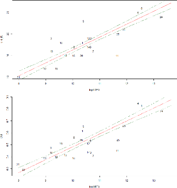
Figure 22: Residuals plots of best GLM: bird species
richness (top row) and log-transformed CSI (bottom row) as a function of the
patches log-transformed area
Some of the patches deviate from the regression line in both
plots (Figure 22). Patches No. 3, 5, 6, 10 and 19 showed higher bird richness
while patches No. 7, 11, 18, 20 and 24 contain lower bird species than the
regression line. Those trends need an interpretation regarding the factors
affecting the deviation of the patches in comparison with the ones situated
along the regression line (patches No. 15, 21, 6,1 for example). The same was
completed with the CSI plot.
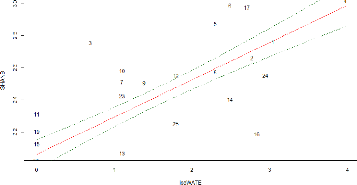
54
Figure 23: Residuals plots of best GLM: Shannon index of bird
diversity as a function the patches log-transformed water cover.
In this case, the patches are more scattered. The patches No.
3 and 16 show both the higher deviance from the regression line, the first one
showing a higher Shannon index of bird diversity and the second showing a lower
one.
V.4.3. Direct gradient analysis
Finally, a redundancy analysis (RDA) was realized with the
ornithological data (abundance matrix) and the environmental factors in order
to identify the relationships between the two data sets.
As we have 10 environmental variables, we have 10 constrained
ordination axes (RDA 1 to RDA 10). In total, the variance explained by the
constrained axes (independent variables, i.e. environmental variables) is equal
to 53% while the rest (47%) is explained by the unconstrained axis (dependent
variables, i.e. bird abundance).
We will focus on the two first axes of the RDA (Figure 24)
that show the highest variance explained in order to simplify the
interpretation. The red names represent each individual species displayed in
the RDA space and the blue vectors show how the environmental variables fall
along that RDA space. The longest vectors along each RDA axis are the most
influent in explaining variation of species abundance along that axis.
The first two constraints axes of the RDA explain respectively
37% and 16 % of the common variance among species and environmental factors (a
total of 53% explained). While those two axes explain respectively 9% and 8% of
the species abundance variance (17% in total). The plot (Figure 24) doesn't
allow us to visualize the actual species impacts on the patches distribution
between the two RDA axes. Regarding the environmental variables, three
variables are negatively correlated (|r|>0.60) with the first axis of the
RDA: logAREA, logWATE and SHANL (Table 12).
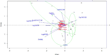
55
Figure 24: Representation of the species abundance and
environmental variables in the plot formed by the two first axes of the RDA.
The green ellipses show the Ward clusters obtained previously. An ellipse
contains 80% of the patches of a group.
The four previous clusters obtained at section IV.4.2 via the
Ward minimum variance method can be visualized on the factorial design shaped
by the two first axes of the RDA (Figure 24). That allows their
characterization. Group 1 and 2 are thus characterized by more open (more
herbaceous and concrete cover), heterogeneous landscapes while group 3 and 4
seem characterized by a more wooded context. Group 2 is elongated by the
spatial variables, situating those patches more in the North of the study area.
They are also characterized by large patches with water.
Table 12: Pearson and Spearman correlation coefficients
between the environmental variables and the two axes of the RDA.
The numbers
highlighted show a correlation with the specified axis.
|
Environmental Factor
|
|
PC1
|
|
P
|
|
PEARSON
|
SPEARMAN
|
PEARSON
|
SPEARMAN
|
|
logAREA
|
-0.858
|
-0.759
|
0.101
|
0.018
|
|
SqrtWCON
|
-0.115
|
0.124
|
0.426
|
0.165
|
|
SqrtSFACTOR
|
-0.439
|
-0.362
|
0.076
|
0.160
|
|
SqrtWOOD
|
0.401
|
0.417
|
0.174
|
0.105
|
|
logHERB
|
-0.487
|
-0.465
|
-0.219
|
-0.158
|
|
logWATE
|
-0.642
|
-0.637
|
-0.005
|
-0.158
|
|
CONC
|
0.016
|
-0.036
|
-0.560
|
-0.540
|
|
SHANL
|
-0.669
|
-0.677
|
-0.382
|
-0.139
|
|
SqrtY3
|
-0.360
|
-0.136
|
0.312
|
0.077
|
|
X3Y3
|
-0.312
|
-0.262
|
0.278
|
0.365
|
56
VI. DISCUSSION
Over the century, as urbanization growth accelerates, urban
green areas are facing severe recession. As the urban sprawl is continually
extending due to land speculation and uncontrolled development, wildlife and
people are getting closer and closer and the conservation of urban biodiversity
emerges as a concern of rising importance (MCKINNEY, 2002).
The potential impact of urbanization on the avifauna has been
largely studied worldwide. However, although Bangkok is a booming megacity
where the environment has been severely damaged, there has not been any
previous studies focusing on the overall urban bird species distribution
(ROUND, 2008). Therefore, this thesis was the timely opportunity to report the
situation of the birds in Central Bangkok so there can be basis implemented for
a future monitoring.
We will guide the discussion through the answers to the two
research questions, namely:
- How is the avifauna characterized and distributed into green
patches situated in the center of the Bangkok Metropolis?
- How do the environmental parameters of those green patches
influence the bird distribution?
In order to best inform the wildlife conservation strategies,
a section regarding the conservation implications will then be highlighted.
Finally, some result need to be nuanced and a section will focus on the
limitations of this study.
HOW IS THE AVIFAUNA CHARACTERIZED AND DISTRIBUTED INTO
GREEN PATCHES SITUATED IN THE CENTER OF THE BANGKOK METROPOLIS?
The results obtained through the ornithological distribution
analysis bring a descriptive overlook of Bangkok's avifauna distribution. Those
results will be discussed together with the literature review statements in
order to be correctly replaced in the thesis context.
Firstly, the bird species sampled (49 species) represented 13
% of the birds assumed to be in the region of the Bangkok Metropolis all year
round (LEPAGE, 2014). This is a quite poor amount but it was predictable as we
focused our study area in the most urbanized part of the city. It confirmed the
statements made by many previous studies, suggesting that species richness
decreases as urban development increases (CHACE and WALSH, 2006; DEVICTOR et
al., 2008; IMAI and NAKASHIZUKA, 2010; MCKINNEY, 2006; NIELSEN et al., 2013;
ORTEGA-ÁLVAREZ and MACGREGOR-FORS, 2009; SANDSTRÖM et al.,
2006).
57
A great part of the bird species found in the green patches
sampled were common native synanthropic species in the Bangkok region like
previously pointed out by ROUND (2008). A great part of those species were
found in the first indicator species group (Table 8), those species being
widespread, often abundant and easily detectable. Those common native species
are of great importance for conservation purpose, since their presence
contributes to the structure, biomass and energy turnover of the environment
they live in (GASTON, 2010). It is all the more important as those species
remain frequent victims of habitat loss as well as species invasion and this
can have deep impacts on their environment and the ecosystem services they
provide. Indeed, the interactions between those common species with city
dwellers can influence positively their wellbeing and increase their relation
with nature (MILLER and HOBBS, 2002). The latter argument is essential because
it brings a socio-economic motivation for the Bangkok administration to invest
in the support of avian biodiversity.
The species abundance structure (Figure 14) showed that most
of the urban species recorded are non-abundant while only a few are very
abundant. Indeed, some species are able to find alternative ecological niches
in the cities and develop quite significant populations alike the common native
synanthropic species listed before. However, those adaptions were also made by
few well known urban-exploiter bird species (native or alien) that created
excessive populations like Columbia Livia (Rock Pigeon, alien) and
Acridotheres tristis (Common Myna, native) pointed out as invasive
species in the GLOBAL INVASIVE SPECIES DATABASE (2005). Today's issue is that
those abundant species tend to become overabundant and create competition with
other native birds, forcing the decreasing of the latter's abundance (CONOLE
and KIRKPATRICK, 2011; DEVICTOR et al., 2008; MCKINNEY, 2006). It is
nevertheless important to nuance the statement that stipulates that a species
is invasive at the whole study area scale. Indeed, even if some species were
more widespread and abundant than others across the whole study area, it would
be essential to look at the invasiveness problem at the patch scale and explore
the metapopulation dynamics (ANDERIES et al., 2007).
The PCoA ordination axes (Figure 18) don't explain a high part
of the variance between the patches regarding their bird assemblages based on
the species abundance. External factors could better explain the bird abundance
distribution within the study area. Indeed, neutral mechanisms like biotic
processes such as scattering or competition, may play a subordinate role in
structuring community composition in urban spaces. According to SATTLER et al.
(2010), human disturbance happening in this case on a regular and frequent
basis by the multiple human activities could cause inhibitions of both the
development and installation of spatially organized biotic processes.
Environmental parameters may play a role as well and their case is discussed
below.
58
HOW DO THE ENVIRONMENTAL PARAMETERS OF THOSE GREEN
PATCHES INFLUENCE THE BIRD DISTRIBUTION?
In order to go further than an assessment of the effect of
urbanization on birds through the creation of species lists and to best inform
wildlife-conservation strategies, it is crucial to understand the
ornithological responses to the modified environmental features of Bangkok.
We know that Bangkok urban green patches are essential to
provide habitat for birds (ROUND, 2008). It is true that the use of a habitat
by a bird differs between every species as well as in between the same species
(FULLER, 2012). However, for conservation purposes, it is important to
attribute the species found in each patch to the way they use their environment
through the evaluation of the observed differences in overall species
abundances. The environmental features investigated in the urban green patches
of central Bangkok supported various bird assemblages that may in part reflect
the availability of different resources. For example, green patches with more
water were more inclined to host bird characteristics of wetlands.
Nevertheless, analyses of community-wide indices are complex to interpret
because they contain a composite response of many individual bird species
(PEARSON, 1993).
The previous tests realized through section V.4 showed that in
the context of Central Bangkok, the size of the patches had the highest
influence on bird species richness and CSI (Figure 22 and Table 11). This
doesn't follow statements made by previous researchers in other regions, which
demonstrated that green patches' internal habitat qualities are of greater
importance than both park size and park isolation for the bird richness and
composition (NIELSEN et al., 2013). We explained the patches showing higher
species richness (or CSI) than the regression line (Figure 22) as being more
heterogeneous patches. The ones below the line, especially patch No. 11 (Sanam
Luang Park) are assumed as being more homogeneous, in this case with a high
herbaceous cover rate.
The bird species heterogeneity (SHANB), on the other hand
(Figure 23), was the most influenced by the rate of water cover in the patches.
In this case, the patches below the regression lines seemed to be homogeneous
but with high wooded cover rates in the case of patch 16, therefore, the
detection of the birds is assumed as poorer than in other patches.
The following paragraphs study separately the environmental
variables types regarding their influence on the ornithological dataset.
- Biogeographic influence
As suggested by other studies as well as by the IBT (
e.g. CASTELLETTA. et al., 2005;
FERNÁNDEZ-JURICIC and JOKIMÄKI, 2001; MACARTHUR and WILSON, 1963,
1967, NIELSEN et al., 2013), a biogeographic variable, the area of the patches,
was the environmental variable affecting the bird richness the most (Figure 22
and Table 11). The area of the patches was also
59
of greatest influence on the bird diversity estimated with the
Shannon index of heterogeneity that takes into account abundance of each
species recorded at one site. Bird communities at a site contained also more
specialized species in larger area patches. The isolation index didn't show
evident influence on the ornithological variables, contrary to what has
previously been predicted by the IBT (MACARTHUR and WILSON, 1963, 1967, NIELSEN
et al., 2013). The possible causes will be later discussed in section
VI.3.3.
- Landscape influence
A first landscape factor explaining highly the bird diversity
was the rate of water cover. It tended to bring more species to the patches
including more wetland specialized species alike Anastomus oscitans
(Asian Openbill), Egretta garzetta (Little Egret), Ardeola
sp. (Pond Heron), Butorides striata (Little heron), or else
,Amaurornis phoenicurus (White-Breasted Waterhen).
Surprisingly, we found a negative influence of the percentage
of wooded cover on the bird species diversity that doesn't corroborates some
previous studies that found that trees play an important role in explaining
urban bird diversity (e.g. EVANS et al., 2009; SANDSTRÖM et al., 2006;
SATTLER et al., 2010). Two reasons can explain those trends; first, the
detectability of birds decreased with an augmentation of wood cover and second,
the larger patches of our study areas were mostly composed of heterogenetic
landscapes while the smaller patches contained merely wood cover.
More herbaceous cover, which was highly correlated with the
Shannon index of landscape heterogeneity seemed to have greater influence on
the more synanthropic group of species (group 1). The concrete cover showed the
same trends but has less influence.
- Spatial influence
The spatial variables don't have an actual influence on the bird
distribution.
Finally, even if environmental variables accounted for a large
percentage of the explanatory power of the bird community models, an important
part of the bird community composition seemed to be determined by environmental
stochasticity, i.e. «random events such as habitat destruction by
human activity, anthropogenic transportation or the introduction of exotic
species» (SATTLER et al., 2010). Environmental variables can explain
some variation in urban bird community composition, however, stochasticity,
appeared to be more important in urban areas than in other habitat types, where
avian species communities are far from stable, enduring constant change while
adapting themselves to the disturbances and changes that constantly modify
their habitat (SATTLER et al., 2010).
60
STUDY LIMITS
As the results obtained before are discussed, it is important
to have a critical subsequent approach on the data quality and directions taken
through the overall thesis.
VI.3.1. Limits regarding the study scope
Due to all of the constraints affecting our green patches
sampling, the patches selected show trends only regarding public areas within
the most urbanized part of Bangkok. Other green patches alike zoos, vacant
lands, privates gardens or street trees haven't been taken into account
although they can be considered as well as green patches and they include
avifauna potential habitat. It is therefore important to ask ourselves the
question of the chosen patches representativeness as they represent only a part
of the green patches within the study area. Furthermore, as the field work
depended on existing structures, the patches didn't range in area and land
cover types and the representativeness of the patches panel can also be
questioned.
VI.3.2. Limits concerning the bird data
collected
A second important fact concerning bird counting is the
difficulty of getting relevant abundance data. Indeed, it has never been
difficult for an ornithologist to create a list of the bird species recorded.
However, calculating species abundance is difficult considering such a mobile
animal. Their mobility could lead us to believe that they could be everywhere
although this is not the case.
It is true that birds are easily seen compared with other taxa
but while counting multi bird species, many studies tend (us also) to assume
them as similar. However, identifying the proximal factor of the urban bird
diversity is relatively difficult as well as studying urbanizations gradients
and biological response because they are far from being linear (MACDONNELL and
HAHS, 2008). Indeed, many parameters affect the bird species differently
according to one species eco-ethology: detectability, response to the
environment changes, adaptation to human disturbances...It is therefore a limit
to assume the anthropic effect or the habitats as equal in the overall patches
while those factors have variable influences for each species. Statistical
models for individual species would be best understood from the perspective of
each species' natural history and habitat preferences but as we focused on the
overall bird distribution and because the number of species was important, we
chose not to proceed in this way (PEARSON, 1993).
Nevertheless, as the study was made in order to implement the
basis for long-term monitoring, the data obtained will be compared to future
data collected in a similar way. Therefore, while forgetting the bias brought
by another observer, the abundance scores specified will allow future surveys
to detect large scale changes in the abundance of individual species.
61
Concerning the identification process, the fact that the field
work was a first ornithological survey experience and, in a foreign country,
and despite the great motivation put into the bird visual and sound
identification, a professional birdwatcher would surely have seen more birds.
Hence, the species identifications we made were accurate concerning the
abundant species while the multiplication of visual encounters allowed us to be
sure of the species recognition. On the other hand, non-abundant less
detectable species can lead to identification mistakes.
VI.3.3. Limits due to the choices of environmental
indices
Some of the previous calculated environmental indices may not
have any impact on the bird distribution. However, it is also possible that the
indices used were not well adapted to the organism studied. For example, the
study of isolation through the calculation of an index of weighted connectivity
has many limits. First, as said before, the patches sampled were not as islands
of habitats surrounded by a hostile urban matrix as presumed through the IBT.
Indeed, street trees or public garden or other habitats could be find inbetween
the patches which brings a relatively high bias to the index calculation.
Second, from one bird species to another, the distances are not assumed as
equal and the study of an isolation index should be done separately for each
species regarding its eco-ethology.
IMPLICATIONS FOR CONSERVATION
«There is no catch-all conservation strategy for
wildlife conservation. Targeting a specific species of concern, a functional
group or the proper response variable will lead to greater gains in comparable
conservation efforts.» (GALITSKY, 2012)
Despite the previous limitations, our study has major
implications to help improve the efficiency of bird conservation efforts in
Bangkok. A geographic layout of the urban biodiversity hotspots was set with
the distribution of the ornithological parameters described throughout this
thesis. To protect, preserve and restore functional green infrastructures in
urban green spaces for birds, large areas should contain compact and clustered
trees separated with sufficient amount and quality of open vegetation and water
inbetween.
However, the implementation of such strategies faces
significant challenges. Increasing the size of existing urban green patches is
difficult, if not impossible in cities. Therefore, strategies to enhance
habitat diversity and resource availability for birds within the patches
appears to be a straightforward way of increasing urban bird diversity.
Furthermore, initiative like the one coming from the Bird
Conservation Society of Thailand, which explored the possibility to implement
an urban bird reserve in eastern Bangkok (ROUND , 2008), should be brought
forward as well.
62
VII. CONCLUSION AND PERSPECTIVES
As there is much concern today about environmental changes, it
is essential to know how those changes affect wildlife over time, and birds
offer a great value as biological and environmental indicators (BIBBY, 1999;
GOTTSCHALK et al., 2005).
This study allowed us to conclude that in Central Bangkok, the
more an urban green space is large and with a heterogeneous landscape, the more
bird species will be numerous and the more specialized species will be found.
The influence of the water cover rates on the species abundance diversity was
demonstrated as well.
The previous results describing the bird distribution are
mostly descriptive and of little use in themselves but will be of high interest
while compared with futures bird counts conducted in a similar way. Indeed,
they will provide a quantification of urban bird diversity evolution across
time since birds are useful indicators of changes within their environment
(BIBBY, 1999; KOSKIMIES, 1989), their quantification is indispensable in order
to implement management measures or to reach a priority for future actions. It
is crucial for the Bangkok government to promote a sustainable development
within the metropolis.
As the landscape is not supposed to change in those green
areas, a landscape monitoring across time doesn't need to be implement.
However, the environmental factors could be complemented by calculating more
intrinsic environment structures within the patches with authorizations and
maps from the BMA and a scale-dependent study could also be apply.
Another clue could be the implementation of volunteer-based
surveys that provide sharing resources to facilitate science and management as
well as an avenue for urban conservation to engage a broader audience. Since
the interest for nature is growing more and more within the inhabitant of
Bangkok (pers. Obs.), initiatives of counting projects from the Bird
Conservation Society of Thailand need to be encouraged and may be
successful.
The development of sustainable cities is today the major goal
for urban landscape planners, government authorities and conservationists (WU,
2009). Programs that aim to find a sustainable balance between the today's
traditional vegetation management and more natural management need to be
implemented in order to contribute to the sustainable efforts (SHWARTZ et al.,
2013). We shall not forget that each city is a unique system and the occurring
management and planning actions should therefore be continuously evaluated to
measure their effectiveness
63
VIII. BIBLIOGRAPHY
ANDERIES J. M., KATTI M. and SHOCHAT E., 2007. Living in the
city: resource availability, predation, and bird population dynamics in urban
areas. Journal of theoretical biology, 247(1),
pp.36-49.
ANDRÉN H., 1994. Effects of habitat fragmentation on
birds and mammals in landscapes with different proportions of suitable habitat:
a review. Oikos, 71, pp.355-366.
ARAÚJO M.B., 2003. The coincidence of people and
biodiversity in Europe. Global Ecology and Biogeography,
12, pp.5-12.
BASTIN L. and THOMAS C.D., 1999. The distribution of plant
species in urban vegetation fragments. Landscape Ecology,
14, pp.493-507.
BEUDELS R. J., 2013. Protected Areas: the best tool we
have against biodiversity loss. Yet, is it enough? Conference at Gembloux
Agro Bio-Tech on October 10th, 2013.
BIBBY C. J. and BUCKLAND S. T., 1987. Bias of bird census
results due to detectability varying with habitat. Acta OEcologica: OEcol.
Gener., 8, pp.103-112.
BIBBY C. J., JONES M. and MARSDEN S., eds., 1998a.
Expedition Field Techniques. Birds Surveys. Geography Outdoors,
London.
BIBBY C. J., MARSDEN S. and FIELDING A., 1998b. Bird-habitat
studies. In: BIBBY C. J., JONES M. and MARSDEN S., eds. Expedition
Field Techniques. Birds Surveys. Geography Outdoors, London. pp.
99-114.
BIBBY C.J., 1999. Making the most of birds as environmental
indicators. Ostrich, 70, pp. 81-88.
BICKFORD D. et al., 2010. Forest Fragment and Breeding Habitat
Characteristics Explain Frog Diversity and Abundance in Singapore.
Biotropica, 42(1), pp.119-125.
BIRDLIFE INTERNATIONAL, 2001. Threatened birds of Asia:
the BirdLife International Red Data Book. Birdlife International,
Cambridge.
BLAIR R.B., 1999. Birds and Butterflies along an Urban
Gradient : Surrogate Taxa for Assessing Biodiversity ? Ecological
Applications, 9(1), pp.164-170.
BOLUND P. and HUNHAMMAR S., 1999. Ecosystem services in urban
areas. Ecol. Econ., 29, pp.293- 301.
64
BRIGGS J. C. 1996. Tropical diversity and conservation.
Conservation Biology, 10, pp. 713-718.
BROWN L.R., 2001. Eco-Economy: Building an Economy for the
Earth. W. W. Norton & Co., New York.
BUREL F. et al., 1999. Ecologie du paysage : concepts,
méthodes et applications. Éd. Tec & doc., Paris.
BURNHAM K. P. and ANDERSON D. R., 2004. Multimodel inference:
Under- standing AIC and BIC in model selection. Sociological methods &
research, 33, pp. 261-304.
CARSON R., 1962. Silent Spring. Riverside Press,
Cambridge.
CASTELLETTA M., THIOLLAY J.-M. and SODHI N. S., 2005. The
effects of extreme forest fragmentation on the bird community of Singapore
Island. Biological Conservation, 121(1),
pp.135-155.
CHACE J. F. and WALSH J. J., 2006. Urban effects on native
avifauna: a review. Landscape and Urban Planning,
74(1), pp.46-69.
CHAN S. et al., 2004. Important Bird Areas in Asia: Key
Sites for Conservation. BirdLife International, Cambridge.
CHOW W.T.L. and ROTH M., 2006. Temporal dynamics of the urban
heat island of Singapore. International Journal of Climatology,
26, pp. 2243-2260.
CLERGEAU P., JOKIMÄKI J. and SAVARD J.-P.L., 2002. Are
urban bird communities influenced by the bird diversity of adjacent landscapes?
Journal of Applied Ecology, 38(5), pp.1122-1134.
COLWELL R. K., 2013. EstimateS: Statistical estimation of
species richness and shared species from samples. Version 9.1.0. User's
Guide and application. «
http://purl.oclc.org/estimates»
(22/07/2014).
CONOLE L.E. and KIRKPATRICK J.B., 2011. Functional and spatial
differentiation of urban bird assemblages at the landscape scale. Landscape
and Urban Planning, 100(1-2), pp.11-23.
DE RIDDER K. et al., 2004. An integrated methodology to assess
the benefits of urban green space. The Science of the total
environment, 334-335, pp.489-497.
DELOYA M.C., 1993. Urban forestry activities in Mexico.
Unasylva, 173(44), pp. 28-32. DEMBNER S.A., 1993.
Urban forestry in Beijing. Unasylva, 173(44), pp.
13-18.
65
DEVICTOR V. et al., 2008. Functional biotic homogenization of
bird communities in disturbed landscapes. Global Ecology and
Biogeography, 17(2), pp.252-261.
DIAMOND J.M., 1975. The island dilemma: lessons of modern
biogeographic studies for the design of natural reserves. Biological
Conservation, 7, pp.129-146.
DOLMAN P.M., 2012. Mechanisms and processes underlying landscape
structure effects on bird populations. In: FULLER R. J., 2012.
Birds and habitat: relationships in changing landscapes. Cambridge
University Press, New York. pp. 93-124.
DUFRÊNE M. and LEGENDRE P., 1997. Species Assemblages and
Indicator Species: The Need for a Flexible Asymmetrical Approach.
Ecological Monographs, 67(3), pp.345-366.
DUFRÊNE M., 2003. Méthodes d'analyse des
données écologiques et biogéographiques. «
http://old.biodiversite.wallonie.be/outils/methodo/»
(24/07/2014)
EVANS K.L., NEWSON S.E. and GASTON K.J., 2009. Habitat
influences on urban avian assemblages. Ibis, 151(1),
pp.19-39.
FAHRIG L., 2003. Effects of habitat fragmentation on
biodiversity. Annual Review of Ecology, Evolution, and Systematics,
34(1), pp.487-515.
FERNÁNDEZ-JURICIC E. and JOKIMÄKI, J., 2001. A
habitat island approach to conserving birds in urban landscapes: case studies
from southern and northern Europe. Biodiversity and Conservation,
10, pp.2023-2043.
FOOD AND AGRICULTURE ORGANIZATION OF THE UNITED NATIONS (FAO),
2012. State of the World's Forests 2012, Food and Agriculture
Organization of the United Nations, Rome, Italy.
FORMAN R.T.T. and GODRON M., 1986. Landscape Ecology.
John Wiley and Sons Inc., New York.
FORMAN R.T.T., 1995. Land mosaics: the ecology of
landscapes and regions. Cambridge University Press, Cambridge.
FRASER E.D.G., 2002. Urban Ecology in Bangkok, Thailand:
Community Participation, Urban Agriculture and Forestry. Environments,
30(1), pp.37-50.
FULLER R. J., ed., 2012. Birds and habitat: relationships
in changing landscapes. Cambridge University Press, New York.
GAILLY R., 2013. Impact des plantations de sapins de
Noël sur l'avifaune des milieux ouverts en Ardenne occidentale.
Travail de fin d'études : Gembloux Agro Bio-Tech/Université de
Liège.
66
GALITSKY C., 2012. Effects of local vegetation and
landscape patterns on avian biodiversity in the threatened oak habitat of the
Willamette Valley, Oregon. Master Thesis: University of Washington.
GASTON K.J., 2010. Valuing Common Species. Science,
327(5962), pp.154-155.
GLOBAL INVASIVE SPECIES DATABASE, 2005. Invasive species
of the organism type bird in Thailand. «
http://www.issg.org/database/species/»
(09/05/2014).
GOTTSCHALK T.K., HUETTMANNJ F. and EHLERS M., 2005. Thirty
years of analyzing and modeling avian habitat relationships using satellite
imagery data: a review. International Journal of Remote Sensing,
26(12), pp.2631-2656.
HELTSHE J.F. and FORRESTER N.E., 1983. Estimating Species
Richness Using the Jackknife Procedure. Biometrics,
39(1), pp.1-11.
HOSTETLER M., 1999. Scale, birds, and human decisions: a
potential for integrative research in urban ecosystems. Landscape and Urban
Planning, 45(1), pp.15-19.
HUSTÉ A. and BOULINIER T., 2011. Determinants of bird
community composition on patches in the suburbs of Paris, France.
Biological Conservation, 144(1), pp.243-252.
IMAI H. and NAKASHIZUKA T., 2010. Environmental factors
affecting the composition and diversity of avian community in mid- to late
breeding season in urban parks and green spaces. Landscape and Urban
Planning, 96(3), pp.183-194.
IUCN, 2013. The IUCN Red List of Threatened Species.
Version 2013.2. «
http://www.iucnredlist.org»
(09/05/2014).
JONES M., 1998. Study design. In: BIBBY C. J., JONES
M. and MARSDEN S., eds. Expedition Field Techniques. Birds Surveys.
Geography Outdoors, London. pp. 15-34.
JULLIARD R. et al., 2006. Spatial segregation of specialists
and generalists in bird communities. Ecology Letters,
9, pp. 1237-1244.
KATTI M. and WARREN P. S., 2004. Tits, noise and urban
bioacoustics. Tree, 19, pp.109-110.
KHEDARI J., SANGPRAJAK A. and HIRUNLABH J., 2002. Thailand
climatic zones. Renewable Energy, 25, pp.267-280.
KHERA N., MEHTA V. and SABATA B.C., 2009. Interrelationship of
birds and habitat features in urban greenspaces in Delhi, India. Urban
Forestry & Urban Greening, 8(3), pp.187-196.
67
KONIJNENDIJK C. C., 2003. A decade of urban forestry in
Europe. Forest Policy and Economics, 5, pp.
175-186.
KOSKIMIES P., 1989. Birds as a tool in environmental
monitoring. Ann. Zool. Fennici, 26, pp.153- 166.
KUCHELMEISTER G., 1998. Urban Forestry: Present Situation
and Prospects in the Asia and Pacific region. FAO Asia-Pacific Forestry
Sector Outlook Study, FAO Working Paper No.: APFSOS/WP/44, Food and Agriculture
Organization of the United Nations, Rome.
KÜHN I., BRANDL R. and KLOTZ S., 2004. The flora of
German cities is naturally species rich. Evolutionary Ecology
Research, 6, pp. 749-764.
LAGHAI H. AND BAHMANPOUR H., 2012. GIS Application in Urban
Green space Per Capita Evaluation (Case study: City of Tehran). Annals of
Biological Research, 3(5),
pp.2439-2446.
LEAKEY R.E. AND LEWIN R., 1999. La sixième
extinction: évolution et catastrophes. Flammarion, Paris.
LEGENDRE P. and LEGENDRE L., 2012. Numerical ecology.
3rd ed., Elsevier, Amsterdam.
LEPAGE D., 2014. Avibase - listes d'oiseaux mondiales :
Bangkok Metropolis. «
http://avibase.bsc-eoc.org/checklist.jsp?region=TH01bm&list=howardmoore»
(10/08/2014).
LIM H.C. and SODHI N.S., 2004. Responses of avian guilds to
urbanisation in a tropical city. Landscape and Urban Planning,
66(4), pp.199-215.
LOUGBEGNON T.O. and CODJIA T.C., 2011. Avifaune urbaine de
Cotonou et sa distribution en relation avec les facteurs de l'habitat:
implications pour l'aménagement écologique de la ville.
Afrique Science, 7(1), pp.116-136.
LUSSENHOP J., 1977. Urban cemeteries as bird refuges. The
Condor, 79, pp.456-461.
MA Z. et al., 2012. Use of localized descriptive statistics for
exploring the spatial pattern changes of bird species richness at multiple
scales. Applied Geography, 32(2), pp.185-194.
MACARTHUR R.H. and WILSON E.O., 1963. An Equilibrium Theory of
Insular Zoogeography. Evolution, 17(4),
pp.373-387.
MACARTHUR R.H. and WILSON E.O., 1967. The Theory of Island
Biogeography. Princeton University Press, Princeton.
68
MACDONNELL M. J. and HAHS A. K., 2008. The use of gradient
analysis studies in advancing our understanding of the ecology of urbanizing
landscapes: current status and future directions. Landscape Ecology,
23, pp.1143-1155
MACGREGOR-FORS I., 2008. Relation between habitat attributes
and bird richness in a western Mexico suburb. Landscape and Urban
Planning, 84(1), pp.92-98.
MARZLUFF J.M., BOWMAN R. and DONNELLY R., 2001. Avian
Ecology and Conservation in an Urbanizing World. Kluwer Academic
Publishers, Dordrecht.
MATEO-BABIANO I.B., 2012. Public life in Bangkok's urban
spaces. Habitat International, 36(4), pp.452-461.
MCKINNEY M.L., 2002. Urbanization, biodiversity, and
conservation. BioScience, 52, pp.883-890.
MCKINNEY M.L., 2006. Urbanization as a major cause of biotic
homogenization. Biological Conservation, 127(3),
pp.247-260.
MILLENNIUM ECOSYSTEM ASSESSMENT (MEA), 2005. Ecosystems
and Human Well-being: Biodiversity Synthesis. World Resources Institute,
Washington.
MILLER J. and HOBBS R., 2002. Conservation where people live
and work. Conservation Biology 16, pp.330-337.
NAPOMPETH B., 2002. Thailand. In: PALLETTAWA N.,
REASER J. K., and GUTIERREZ A. T., eds. Invasive Alien Species in
South-Southeast Asia: National Reports & Directory of Resources. pp.
104-106.
NIELSEN A.B. et al., 2013. Species richness in urban parks and
its drivers: A review of empirical evidence. Urban Ecosystems,
17(1), pp.305-327.
ORTEGA-ÁLVAREZ R. and MACGREGOR-FORS I., 2009. Living
in the big city: Effects of urban land-use on bird community structure,
diversity, and composition. Landscape and Urban Planning,
90(3-4), pp.189-195.
PEARSON S.M., 1993. The spatial extent and relative influence
of landscape-level factors on wintering bird populations '. Landscape
Ecology, 8(1), pp.3-18.
POMEROY D., 1992. Counting Birds. A guide to assessing
numbers, biomass and diversity of Afrotropical birds. AWF, Nairobi.
69
PURVIS A. and HECTOR A., 2000. Getting the measure of
biodiversity. Nature, 405(6783), pp.212- 219.
RAMALHO C.E. and HOBBS R.J., 2012. Time for a change: dynamic
urban ecology. Trends in ecology & evolution,
27(3), pp.179-88.
ROBERTS D. W., 2010. Ordination and Multivariate Analysis
for Ecology. «
http://ecology.msu.montana.edu/labdsv/R/»
(23/07/2014).
ROBERTSON P. A. and LILEY D., 1998. Assessment of sites:
Measurement of species richness and diversity. In: BIBBY C. J., JONES
M. and MARSDEN S., eds. Expedition Field Techniques. Birds Surveys.
Geography Outdoors, London. pp. 76-98.
ROBSON C., 2002. Birds of Thailand. Princeton
University Press, Princeton.
ROSENZWEIG M.L., 2003. Win-Win Ecology: How Earth's
Species can Survive in the Midst of Human Enterprise. Oxford University
Press, New York.
ROUND P., 2008. The birds of the Bangkok area, White
Lotus Press, Bangkok.
ROYSTON P., 1982. Algorithm AS 181: The W test for Normality.
Applied Statistics, 31, pp. 176- 180.
SANDSTRÖM U. G., ANGELSTAM P. and MIKUSIÑSKI G.,
2006. Ecological diversity of birds in relation to the structure of urban green
space. Landscape and Urban Planning, 77(1-2),
pp.39-53.
SATTLER T. et al., 2010. Spider, bee, and bird communities in
cities are shaped by environmental control and high stochasticity.
Ecology, 91(11), pp.3343-53.
SAVARD J.-P.L., CLERGEAU P. and MENNECHEZ G., 2000.
Biodiversity concepts and urban ecosystems. Landscape and Urban
Planning, 48(3-4), pp.131-142.
SAX D.F. and GAINES S.D., 2003. Species diversity: from global
decreases to local increases. Trends in Ecology & Evolution,
18(11), pp.561-566.
SHANNON C.E., 1948. A mathematical theory of communication.
Bell System Technical Journal, 27, pp. 379-423.
SHWARTZ A., MURATET A., SIMON L. and JULLIARD R., 2013. Local
and management variables outweigh landscape effects in enhancing the diversity
of different taxa in a big metropolis. Biological Conservation,
157, pp. 285-292.
70
SINGH V. S., PANDEY D. N. and CHAUDHRY P., 2010. Urban
forests and open green spaces: lessons for Jaipur, Rajasthan, India.
Occasional paper from the Rajasthan State Pollution Control Board.
SODHI N.S. and BROOK B.W., 2006. Southeast Asian
Biodiversity in Crisis. Cambridge University Press, Cambridge.
SODHI N.S. and LIOW L.H., 2000. Improving Conservation Biology
Research in Southeast Asia, Conservation Biology,
14(4), pp.1211-1212.
SODHI N.S. et al., 1999. Bird use of linear areas of a
tropical city: implications for park connector design and management.
Landscape and Urban Planning, 45(2-3), pp.123-130.
SODHI N.S. et al., 2004. Southeast Asian biodiversity: an
impending disaster. Trends in ecology and evolution,
19(12), pp.654-660.
SODHI N.S. et al., 2009. The state and conservation of
Southeast Asian biodiversity. Biodiversity and Conservation,
19(2), pp.317-328.
SODHI N.S., KOH L.P. and BROOK B.W., 2006. Southeast Asian
birds in peril. The Auk, 123(1), pp.275-277.
SORACE A., 2002. High density of bird and pest species in
urban habitats and the role of predator abundance. Ornis Fenn.
79, pp.60-71.
SPELLERBERG I.A.N.F. and FEDOR P.J., 2003. A tribute to Claude
Shannon (1916 - 2001) and a plea for more rigorous use of species richness,
species diversity and the « Shannon - Wiener» Index. Global
Ecology and Biogeography, 12, pp.177-179.
THAIUTSA B. et al., 2008. Urban green space, street tree and
heritage large tree assessment in Bangkok, Thailand. Urban Forestry &
Urban Greening, 7, pp.219-229
TURNER W. R., 2003. Citywide biological monitoring as a tool
for ecology and conservation in urban landscapes: the case of the Tucson Bird
Count. Landscape and Urban Planning, 65(3),
pp.149-166.
UNITED NATIONS (UN), DEPARTMENT OF ECONOMIC AND SOCIAL
AFFAIRS, POPULATION DIVISION, 2012. World Urbanization Prospects: The 2011
Revision: Highlights. New York.
UNITED NATIONS CONFERENCE ON ENVIRONMENT AND DEVELOPMENT
(UNCED), 5th of June 1992. Convention on Biological
Diversity, Rio de Janeiro. 1760 UNTS 79; 31 ILM 818.
71
VAN TURNHOUT C. A. M. et al., 2007. Scale-dependent
homogenization: Changes in breeding bird diversity in the Netherlands over a
25-year period. Biological Conservation, 134(4),
pp.505- 516.
WHITE E.P. and HURLBERT A.H., 2010. The combined influence of
the local environment and regional enrichment on bird species richness. The
American naturalist, 175(2), pp.E35-E43.
WHITE J.G. et al., 2005. Non-uniform bird assemblages in urban
environments: the influence of streetscape vegetation. Landscape and Urban
Planning, 71(2-4), pp.123-135.
WHITTINGHAM M. J., STEPHENS P. A., BRADBURY R.B. and
FRECKLETON R.P., 2006. Why do we still use stepwise modelling in ecology and
behaviour? Journal of Animal Ecology, 75, pp. 1182- 1189.
WILLIAMS J.N., 2012. Humans and biodiversity: population and
demographic trends in the hotspots. Population and Environment,
34(4), pp.510-523.
WORLD HEALTH ORGANIZATION (WHO), 2008. Our cities, our health,
our future. Report to the WHO Commission on Social Determinants of Health
from the Knowledge Network on Urban Settings.
WU J., 2009. Urban sustainability: an inevitable goal of
landscape research. Landscape Ecology, 25(1),
pp.1-4.
i
APPENDICES
APPENDIX 1: GAZETTEER OF THE GREEN PATCHES SAMPLED II
APPENDIX 2: BIRD LIST AND SEASONAL STATUS III
APPENDIX 3: PUNCTUAL RICHNESS COMPARED WITH THE RICHNESS
OBSERVED IN THE MORNING AND IN THE AFTERNOON V
APPENDIX 4: COMPARISON BETWEEN THE PATCHES REGARDING THEIR
ORNITHOLOGICAL CHARACTERISTICS. VI
APPENDIX 5: CORRELATION MATRIX OF THE ENVIRONMENTAL VARIABLES
VII
APPENDIX 6: COMPARISON BETWEEN THE PATCHES REGARDING THEIR
ENVIRONMENTAL CHARACTERISTICS VIII
|
APPENDIX 1: GAZETTEER OF THE GREEN PATCHES
SAMPLED
|
|
|
|
PATCH N°
|
Name
|
Type
|
Longitude
|
Latitude8
|
|
1
|
Somdet Saranrat Maneerom Park
|
Park
|
100.590320
|
13.742434
|
|
2
|
Benjasiri Park
|
Park
|
100.567424
|
13.730513
|
|
3
|
Chuvit Garden
|
Park
|
100.557054
|
13.738443
|
|
4
|
Benjakitti Park
|
Park
|
100.558569
|
13.729384
|
|
5
|
Santiphap Park
|
Park
|
100.541323
|
13.762778
|
|
6
|
Chatuchak Park
|
Park
|
100.553783
|
13.804674
|
|
7
|
Pathum Wanaram Temple
|
Temple
|
100.536832
|
13.746267
|
|
8
|
Phanphirom Park
|
Park
|
100.591922
|
13.751225
|
|
9
|
Romaneenaart Park
|
Park
|
100.502551
|
13.749001
|
|
10
|
Santichai Prakan Public Park
|
Park
|
100.495482
|
13.764088
|
|
11
|
Sanam Luang Park
|
Park
|
100.493086
|
13.755204
|
|
12
|
Saranrom Park
|
Park
|
100.495169
|
13.748316
|
|
13
|
Nagaraphirom Park
|
Park
|
100.490174
|
13.746893
|
|
14
|
No Name
(under Sirat Expressway)
|
Park
|
100.549435
|
13.757224
|
|
15
|
No Name
(under Chalerm Maha Nakhorn Expressway)
|
Park
|
100.544085
|
13.758199
|
|
16
|
Vibhavadi Rangsit Forest Park
|
Park
|
100.553345
|
13.772275
|
|
17
|
Rot Fai and Queen Sirikit Park
|
Park
|
100.553254
|
13.811215
|
|
18
|
Princess Mother Garden
|
Park
|
100.560002
|
13.814623
|
|
19
|
Next to BTS Sathorn
|
Park
|
100.514444
|
13.718354
|
|
20
|
Chaloemprakiarti Forest Park
|
Park
|
100.510479
|
13.719703
|
|
21
|
No Name
Next to BTS Thonburi (North)
|
Crossroad greenery
|
100.505818
|
13.721150
|
|
22
|
No Name
Next to BTS Thonburi (South)
|
Crossroad greenery
|
100.505906
|
13.720329
|
|
23
|
Tae Chio Cemetery
|
Cemetery
|
100.523947
|
13.714271
|
|
24
|
Lumphini Park
|
Park
|
100.541316
|
13.730972
|
|
25
|
Chulalongkorn University
|
University
|
100.530864
|
13.738592
|
ii
8 Longitude and Latitude are those of the approximate
center of the green patches in decimal degrees
iii
APPENDIX 2: BIRD LIST AND SEASONAL STATUS
Seasonal status is indicated as follows (ROUND, 2008):
R= Resident or presumed resident
N= Non-breeding visitor
P= Passage Migrant
E= Presumed escaped captives (pers. obs.)
Kept for the analyses
Species Common english name Seasonal status
Acridotheres grandis White-vented Myna R
Acridotheres tristis Common Myna R
Aegithina tiphia Common Iora R
Amaurornis phoenicurus White-Breasted Waterhen R
Anastomus oscitans Asian Openbill R
Anthreptes malacensis Brown-Throated Sunbird R
Apus nipalensis House swift. R
Ardeola sp.9 Pond Heron sp. R
Butorides striata Little heron R
Cacomantis merulinus Plaintive Cuckoo R
Centropus sinensis Greater Coucal R
Columba livia Rock Pigeon R
Copsychus saularis Oriental Magpie Robin R
Coracias benghalensis Indian Roller R
Coracina melaschistos Black-winged Cuckooshrike N
Corvus macrorhynchos Large-Billed Crow R
Dicaeum cruentatum Scarlet-Backed Flowerpecker R
Dicrurus macrocercus Ashy Drongo N
Egretta garzetta Little Egret R
Eudynamys scolopaceus Asian Koel R
Ficedula albicilla Red-throated Flycatcher N
Garrulax leucolophus White-crested Laughingthrush E
Geopelia striata Zebra Dove R
Hirundo rustica Barn Swallow N
Lanius cristatus Brown Shrike N
Lonchura punctulata Scaly-breasted Munia R
9 The non-breeding plumage of the Javan, Chinese
and Indian pond herons are similar and virtually indistinguishable in the
field. Furthermore, some hybrids have been observed by local birdwatchers.
Megalaima haemacephala Coppersmith Barbet R
iv
Merops sp.10 Bee-eater sp. P
Muscicapa dauurica Asian Brown Flycatcher N
Muscicapa sibirica Dark-sided Flycatcher P
Nectarinia jugularis Olive-Backed Sunbird R
Ninox scutulata Brown Boobook N
Oriolus chinensis Black-Naped Oriole N
Orthotomus sutorius Common Tailorbird R
Passer domesticus House Sparrow R
Passer flaveolus Plain-backed Sparrow R
Passer montanus Eurasian Tree Sparrow R
Pericrocotus cinnamomeus Small Minivet R
Phylloscopus inornatus Yellow-Browed Warbler N
Psittacula alexandri Red-Breasted Parakeet E
Pycnonotus blanfordi Streak-Eared Bulbul R
Pycnonotus goiavier Yellow-Vented Bulbul R
Pycnonotus jocosus Red-Whiskered Bulbul E
Rhipidura javanica Pied Fantail R
Streptopelia chinensis Spotted Dove R
Streptopelia tranquebarica Red Collared Dove R
Sturnus contra Asian Pied Starling R
Sturnus nigrocollis Black-Collared Starling R
Treron sp.11 Green Pigeon sp. E
10 Too far to be well identified. Presumed as being
Merops philippinus (Blue-tailed Bee-eater)
11 Too far to be well identified. Presumed as being
Treron curvirostra (Thick-billed Green Pigeon)
V
APPENDIX 3: PUNCTUAL RICHNESS COMPARED WITH THE
RICHNESS OBSERVED IN THE MORNING AND IN THE AFTERNOON
|
Patch n°
|
|
Punctual Richness
|
|
|
|
Morning
|
|
|
Afternoon
|
|
|
Average
|
S. D.
|
Minimum
|
Maximum
|
Average
|
S. D.
|
Minimum
|
Maximum
|
Average
|
S. D.
|
Minimum
|
Maximum
|
|
1
|
14.3
|
1.75
|
11
|
16
|
15.0
|
1.00
|
14
|
16
|
13.7
|
2.31
|
11
|
15
|
|
2
|
14.0
|
0.89
|
13
|
15
|
14.3
|
0.58
|
14
|
15
|
13.7
|
1.15
|
13
|
15
|
|
3
|
14.0
|
1.79
|
11
|
16
|
15.3
|
0.58
|
15
|
16
|
12.7
|
1.53
|
11
|
14
|
|
4
|
20.5
|
2.43
|
17
|
24
|
22.3
|
1.53
|
21
|
24
|
18.7
|
1.53
|
17
|
20
|
|
5
|
17.3
|
1.97
|
15
|
19
|
19.0
|
0.00
|
19
|
19
|
15.7
|
1.15
|
15
|
17
|
|
6
|
22.2
|
1.60
|
20
|
24
|
22.3
|
1.53
|
21
|
24
|
22.0
|
2.00
|
20
|
24
|
|
7
|
12.7
|
1.86
|
10
|
15
|
12.7
|
2.52
|
10
|
15
|
12.7
|
1.53
|
11
|
14
|
|
8
|
11.2
|
1.47
|
10
|
14
|
12.0
|
1.73
|
11
|
14
|
10.3
|
0.58
|
10
|
11
|
|
9
|
12.5
|
2.66
|
9
|
16
|
14.7
|
1.15
|
14
|
16
|
10.3
|
1.53
|
9
|
12
|
|
10
|
14.2
|
1.60
|
11
|
15
|
15.0
|
0.00
|
15
|
15
|
13.3
|
2.08
|
11
|
15
|
|
11
|
11.5
|
2.26
|
8
|
14
|
12.7
|
1.53
|
11
|
14
|
10.3
|
2.52
|
8
|
13
|
|
12
|
13.2
|
1.72
|
11
|
16
|
14.3
|
1.53
|
13
|
16
|
12.0
|
1.00
|
11
|
13
|
|
13
|
7.2
|
0.98
|
6
|
8
|
8.0
|
0.00
|
8
|
8
|
6.3
|
0.58
|
6
|
7
|
|
14
|
14.0
|
1.41
|
12
|
16
|
15.0
|
1.00
|
14
|
16
|
13.0
|
1.00
|
12
|
14
|
|
15
|
8.8
|
2.48
|
6
|
13
|
10.7
|
2.08
|
9
|
13
|
7.0
|
1.00
|
6
|
8
|
|
16
|
12.0
|
2.10
|
9
|
15
|
13.7
|
1.15
|
13
|
15
|
10.3
|
1.15
|
9
|
11
|
|
17
|
26.5
|
1.22
|
25
|
28
|
26.7
|
1.53
|
25
|
28
|
26.3
|
1.15
|
25
|
27
|
|
18
|
7.2
|
1.17
|
6
|
9
|
8.0
|
1.00
|
7
|
9
|
6.3
|
0.58
|
6
|
7
|
|
19
|
9.5
|
1.64
|
7
|
11
|
10.3
|
0.58
|
10
|
11
|
8.7
|
2.08
|
7
|
11
|
|
20
|
8.7
|
2.66
|
6
|
12
|
11.0
|
1.00
|
10
|
12
|
6.3
|
0.58
|
6
|
7
|
|
21
|
5.8
|
1.83
|
4
|
9
|
7.0
|
2.00
|
5
|
9
|
4.7
|
0.58
|
4
|
5
|
|
22
|
4.8
|
1.72
|
3
|
7
|
5.0
|
1.73
|
4
|
7
|
4.7
|
2.08
|
3
|
7
|
|
23
|
15.5
|
1.22
|
14
|
17
|
16.3
|
1.15
|
15
|
17
|
14.7
|
0.58
|
14
|
15
|
|
24
|
20.5
|
1.87
|
18
|
23
|
20.3
|
1.53
|
19
|
22
|
20.7
|
2.52
|
18
|
23
|
|
25
|
13.8
|
1.17
|
12
|
15
|
13.7
|
1.53
|
12
|
15
|
14.0
|
1.00
|
13
|
15
|
vi
APPENDIX 4: COMPARISON BETWEEN THE
CHARACTERISTICS.
|
PATCHES REGARDING THEIR ORNITHOLOGICAL
|
|
Patch
n°
|
bird_R
|
Total sum of
Abundance scores
|
Average
Abundance score
|
Shannon
Index
|
CSI
|
|
1
|
18
|
54
|
3.2
|
2.764
|
0.616
|
|
2
|
19
|
51
|
3.2
|
2.663
|
0.435
|
|
3
|
19
|
57
|
3.2
|
2.756
|
0.476
|
|
4
|
25
|
65
|
2.6
|
3.018
|
0.807
|
|
5
|
23
|
60
|
2.7
|
2.875
|
0.655
|
|
6
|
26
|
69
|
2.8
|
2.990
|
0.828
|
|
7
|
16
|
51
|
3.2
|
2.513
|
0.407
|
|
8
|
17
|
49
|
2.7
|
2.574
|
0.743
|
|
9
|
17
|
51
|
3.0
|
2.508
|
0.534
|
|
10
|
18
|
61
|
3.4
|
2.583
|
0.512
|
|
11
|
15
|
45
|
3.0
|
2.312
|
0.451
|
|
12
|
19
|
57
|
3.0
|
2.552
|
0.512
|
|
13
|
12
|
40
|
3.3
|
2.069
|
0.389
|
|
14
|
17
|
55
|
3.2
|
2.406
|
0.438
|
|
15
|
15
|
41
|
2.7
|
2.128
|
0.414
|
|
16
|
15
|
44
|
2.9
|
2.189
|
0.388
|
|
17
|
31
|
88
|
2.8
|
2.978
|
1.128
|
|
18
|
12
|
37
|
3.1
|
1.913
|
0.399
|
|
19
|
16
|
49
|
3.1
|
2.205
|
0.436
|
|
20
|
15
|
37
|
2.5
|
2.025
|
0.540
|
|
21
|
10
|
33
|
3.3
|
1.698
|
0.337
|
|
22
|
9
|
29
|
3.2
|
1.559
|
0.290
|
|
23
|
21
|
63
|
3.0
|
2.425
|
0.660
|
|
24
|
24
|
72
|
3.0
|
2.554
|
0.782
|
|
25
|
20
|
58
|
2.9
|
2.253
|
0.542
|
vii
APPENDIX 5: CORRELATION MATRIX OF THE ENVIRONMENTAL
VARIABLES
Cell content: Pearson's correlation (P-value) Highlighted:
correlated variables (>0.7)
|
AREA
|
AREA
1
|
WCON
|
SFACTOR
|
WOOD
|
HERB
|
WATE
|
CONC
|
nLC
|
SHANL
|
X
|
Y
|
X2
|
Y2
|
XY
|
X2Y
|
XY2
|
X2+Y2
|
|
|
WCON
|
0.135732
|
1
|
|
|
|
|
|
|
|
|
|
|
|
|
|
|
|
|
|
SFACTOR
|
0.262775
|
0.52926
|
1
|
|
|
|
|
|
|
|
|
|
|
|
|
|
|
|
|
T
|
-0.2771
|
-0.23593
|
-0.44805
|
1
|
|
|
|
|
|
|
|
|
|
|
|
|
|
|
|
H
|
0.285552
|
0.441068
|
0.466348
|
-0.64643
|
1
|
|
|
|
|
|
|
|
|
|
|
|
|
|
|
W
|
0.380991
|
0.005337
|
0.191331
|
-0.35113
|
-0.10492
|
1
|
|
|
|
|
|
|
|
|
|
|
|
|
|
C
|
-0.18488
|
-0.10499
|
0.044278
|
-0.5801
|
-0.01223
|
-0.10255
|
1
|
|
|
|
|
|
|
|
|
|
|
|
|
nLC
|
0.221454
|
0.050828
|
0.518043
|
-0.65548
|
0.226946
|
0.335523
|
0.510409
|
1
|
|
|
|
|
|
|
|
|
|
|
|
SHANL
|
0.384442
|
0.054317
|
0.503373
|
-0.82851
|
0.436065
|
0.404938
|
0.494844
|
0.880369
|
1
|
|
|
|
|
|
|
|
|
|
|
X
|
0.180658
|
0.179194
|
0.293032
|
-0.13948
|
-0.06559
|
0.502741
|
-0.10811
|
0.329612
|
0.379773
|
1
|
|
|
|
|
|
|
|
|
|
Y
|
0.33663
|
0.542504
|
0.422484
|
-0.07662
|
0.191201
|
0.016192
|
-0.09327
|
0.219783
|
0.156515
|
0.282855
|
1
|
|
|
|
|
|
|
|
|
X2
|
0.180614
|
0.179171
|
0.292999
|
-0.13951
|
-0.06558
|
0.502736
|
-0.10807
|
0.32961
|
0.379793
|
1
|
0.282844
|
1
|
|
|
|
|
|
|
|
Y2
|
0.337018
|
0.542869
|
0.422473
|
-0.07638
|
0.191281
|
0.016144
|
-0.09369
|
0.219376
|
0.156143
|
0.282869
|
0.999999
|
0.282858
|
1
|
|
|
|
|
|
|
XY
|
0.345552
|
0.541243
|
0.442938
|
-0.09234
|
0.172704
|
0.085725
|
-0.10392
|
0.255137
|
0.201966
|
0.409065
|
0.990947
|
0.409054
|
0.990949
|
1
|
|
|
|
|
|
X2Y
|
0.348224
|
0.53183
|
0.454423
|
-0.10498
|
0.153543
|
0.14652
|
-0.11184
|
0.282811
|
0.239478
|
0.515537
|
0.967697
|
0.515527
|
0.967701
|
0.992784
|
1
|
|
|
|
|
XY2
|
0.342356
|
0.543469
|
0.43392
|
-0.08459
|
0.182216
|
0.051828
|
-0.09938
|
0.237973
|
0.179775
|
0.348254
|
0.997624
|
0.348243
|
0.997626
|
0.997841
|
0.982765
|
1
|
|
|
|
X2+Y2
|
0.214244
|
0.237966
|
0.332403
|
-0.14306
|
-0.03954
|
0.483911
|
-0.11503
|
0.342731
|
0.383126
|
0.993136
|
0.3931
|
0.993135
|
0.393113
|
0.512986
|
0.61222
|
0.455505
|
1
|
|
|
X3
|
0.18057
|
0.179148
|
0.292965
|
-0.13955
|
-0.06556
|
0.502731
|
-0.10804
|
0.329608
|
0.379812
|
1
|
0.282833
|
1
|
0.282847
|
0.409043
|
0.515517
|
0.348232
|
0.993134
|
|
|
Y3
|
0.337406
|
0.543234
|
0.422461
|
-0.07615
|
0.191361
|
0.016096
|
-0.0941
|
0.218969
|
0.155771
|
0.282884
|
0.999997
|
0.282872
|
0.999999
|
0.990949
|
0.967703
|
0.997626
|
0.393127
|
0.
|
|
X3+Y3
|
0.185507
|
0.187659
|
0.29881
|
-0.14016
|
-0.06191
|
0.500477
|
-0.10913
|
0.331742
|
0.380597
|
0.999862
|
0.298736
|
0.999862
|
0.29875
|
0.424153
|
0.529688
|
0.363765
|
0.994941
|
0.
|
WOOD
Patch n° AREA WCON SFACTOR 0 ER ÿ SHANL
Y3 X3+Y3 ON
HERB
WATE
CONC
viii
APPENDIX 6: COMPARISON BETWEEN THE PATCHES REGARDING
THEIR ENVIRONMENTAL CHARACTERISTICS
|
1
|
31630
|
1.92E-04
|
1.311
|
41
|
9
|
20
|
30
|
1.266
|
2595.32
|
1020410
|
|
2
|
43382
|
3.67E-04
|
1.343
|
55
|
6
|
15
|
24
|
1.122
|
2588.57
|
1019708
|
|
3
|
9849
|
5.49E-04
|
1.175
|
63
|
12
|
1
|
23
|
0.945
|
2593.06
|
1019398
|
|
4
|
247213
|
3.60E-04
|
1.266
|
28
|
3
|
52
|
18
|
1.097
|
2587.93
|
1019439
|
|
5
|
32738
|
3.29E-04
|
1.804
|
58
|
6
|
9
|
28
|
1.057
|
2606.86
|
1018935
|
|
6
|
284069
|
6.59E-02
|
2.231
|
16
|
54
|
11
|
20
|
1.185
|
2630.74
|
1019336
|
|
7
|
47085
|
4.54E-04
|
1.182
|
52
|
0
|
2
|
46
|
0.785
|
2597.49
|
1018789
|
|
8
|
23209
|
1.92E-04
|
1.377
|
35
|
23
|
9
|
32
|
1.292
|
2600.30
|
1020463
|
|
9
|
42631
|
2.66E-04
|
1.242
|
67
|
7
|
3
|
24
|
0.896
|
2599.04
|
1017751
|
|
10
|
14217
|
2.52E-04
|
1.369
|
46
|
13
|
2
|
39
|
1.071
|
2607.61
|
1017546
|
|
11
|
114859
|
2.29E-04
|
1.376
|
26
|
55
|
0
|
20
|
1.001
|
2602.56
|
1017468
|
|
12
|
39042
|
3.19E-04
|
1.062
|
70
|
5
|
5
|
20
|
0.867
|
2598.65
|
1017527
|
|
13
|
7805
|
2.81E-04
|
1.056
|
19
|
20
|
2
|
59
|
1.034
|
2597.85
|
1017375
|
|
14
|
39005
|
3.36E-04
|
1.180
|
35
|
15
|
11
|
39
|
1.268
|
2603.71
|
1019178
|
|
15
|
16701
|
3.29E-04
|
1.263
|
79
|
7
|
0
|
14
|
0.653
|
2604.26
|
1019016
|
|
16
|
22681
|
3.76E-04
|
1.858
|
75
|
1
|
16
|
8
|
0.754
|
2612.26
|
1019305
|
|
17
|
835221
|
2.99E-04
|
1.582
|
50
|
21
|
14
|
14
|
1.228
|
2634.48
|
1019324
|
|
18
|
11964
|
2.25E-02
|
1.066
|
86
|
0
|
1
|
14
|
0.439
|
2636.44
|
1019531
|
|
19
|
9920
|
3.96E-03
|
1.638
|
49
|
12
|
0
|
39
|
0.997
|
2581.70
|
1018095
|
|
20
|
30445
|
3.38E-04
|
1.336
|
52
|
2
|
0
|
46
|
0.767
|
2582.46
|
1017975
|
|
21
|
2929
|
2.74E-04
|
0.862
|
100
|
0
|
0
|
0
|
0.000
|
2583.28
|
1017835
|
|
22
|
3546
|
3.67E-04
|
0.783
|
100
|
0
|
0
|
0
|
0.000
|
2582.82
|
1017837
|
|
23
|
146990
|
3.05E-04
|
1.459
|
41
|
47
|
2
|
9
|
1.023
|
2579.40
|
1018380
|
|
24
|
586824
|
3.08E-04
|
1.217
|
44
|
14
|
18
|
24
|
1.289
|
2588.83
|
1018916
|
|
25
|
118390
|
2.69E-04
|
1.287
|
51
|
16
|
5
|
28
|
1.132
|
2593.14
|
1018604
|
| 

