Memoire Online - A study of the birds in central Bangkok (Thailand) in order to implement the basis of a long term monitoring

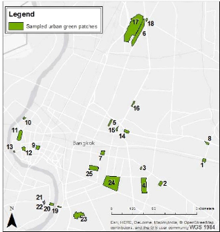
As a reminder, the goal of this study is to investigate the ornithological characteristics, together with the environmental factors affecting them, within various vegetation patches in Bangkok in order to implement the basis for a long term monitoring.

In order to reach the fixed goal, a suite of processes was followed. First, the vegetation patches were sampled within the study area. A field phase was then realized within those green patches to collect the raw ornithological data. On the other hand, the environmental data were obtained from a digitalization out of satellite imagery using the GIS software ArcGIS(c) 10.1. Various variables were then calculated to permit the description of the urban green patches' ornithological and environmental characteristics. Different statistical methods (principally multivariate) were finally used in order to point out the bird communities formed and how the environmental features affect them.

The three main components of a landscape structure are (FORMAN and GODRON, 1986):

- The patches: functional units of the landscape which represent homogeneous environmental conditions and whose boundaries are distinguished by discontinuities in the state variable of a significant magnitude for the ecological process or the considered organism. All patches showing similar characteristics for the considered process is called «type» or «class».

- The corridors: units of a characteristic linear form. The «corridors» perform the ecological function of passage, filter or barrier. They are often present in a network-like landscape.

- The matrix: across types, the «matrix» is the most common and the less fragmented. This type can also be considered as the background of the landscape within which are situated the other elements.

This work will focus on the birds of the «urban green» patch type, the matrix in this case being the concrete of the urban zone. Unfortunately, the avian distribution in the corridors won't be approached because of the lack of time, although it can hold a high level of bird diversity (SODHI et al., 1999; WHITE et al., 2005).

The precise localization of the green spaces in the study area was a first necessary component for the proper achievement of the sampling. Like many cities, Bangkok has spatially explicit planning, land use, and land cover maps for the entire city. Regrettably, it was not possible to get those maps, especially in the context of the political crisis that occurred during the time of the field work.

A digitalization of those green patches was made possible thanks to the interpretation given out of Google Earth(c) satellite imagery (version 7.1.2.2041, accessed on February 2014), Google Maps(c) and various recent tourist maps of the city. A preliminary process of exploration was achieved ten days before the start of the survey to validate in the field the potential green areas.

Some factors affected the selection of the parks and restricted the sampling possibilities:

- we focused on green areas localized in the most densely urbanized area of the city - all the green patches of Bangkok were not open to public

Finally, we selected 25 green patches on a total sampling basis, which means that all the green areas identified accessible and public allowed were designated for the study. Most of them were urban public parks, with two crossroad greeneries, one temple, one University's park, and adding to that, a cemetery (Appendix 1). As we realized the study in all public areas, we assumed the anthropic effect as equal. Furthermore, as poacher's activities are unobserved and because people don't really hunt birds in the city (ROUND, 2008), the presence of people will not reduce the bird presence but is more likely to affect our chances to detect them.

Ideally, the order of visit of the different parks should be determined on a random basis. However, practically, in order to optimize the movements across the study area, small green patches, close to each other were all visited within a same survey period. Because some species have a more active acoustic activity in the early morning, the order of visit into the parks surveyed together was inversed every day. Thus, a green patch visited in the early morning one day, was visited at the end of the morning the next day in order to increase the probability of encountering all the present species. The same scheme was followed for the afternoon.

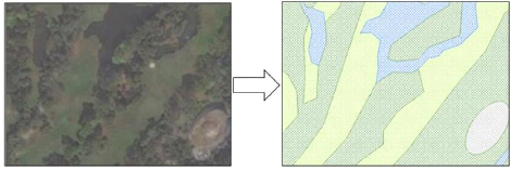
Figure 7: Map of the patches sampled in Central Bangkok RAW DATA COLLECTION

Counting the avian fauna can get quite complex and a review of the literature provides plenty of methods that were employed to do it (POMEROY, 1992). According to JONES (1998), «It is better to get reliable data using a simple method than unreliable data from a complex one, even if the latter (potentially at least) could provide more information». The major reason for adopting a simpler method is to make it easily repeatable, i.e. it allows the study to be significant even if the operators are different, don't have the same level of training or don't put the same amount of effort in the study (JONES, 1998). It is all the more important for this study as it implements the basis for a long term monitoring and others will repeat this work in the future.

The two basics aspects of counting birds are the number of species and the number of individuals (POMEROY, 1992). We will record both while making counts, but they are not necessarily related. Indeed, the importance of birds in the ecosystem varies from place to place because different places have variable numbers of species and individuals (POMEROY, 1992).

The counting method depends upon many things, such as why the counting is made, which level of accuracy needs to be achieved, which resource is available and what time of the day and of the year the survey is done (POMEROY, 1992). Moreover, many factors affect bird activity and behavior, which influences the chances of recording them. Among the more important factors are the season, the time of the day and weather condition (JONES, 1998).

Seasonal effects on birds can be difficult to cope with. JONES (1998) shows the case of a species which is breeding: while the males may be singing and calling to defend their territory, which makes it easy to record them, the females that are nesting won't be seen.

The ornithologist survey we realized within the field phase took place between February 17^th and June 4^th 2014 i.e. during Thailand's hot season. As it was spread over a short period of time, the seasonal effect was minimized. However, as the migration period occurred in April-May, and the non-breeding visitors leave Bangkok around this time as well, the bird's seasonal status (ROUND, 2008) were recorded on the bird species list created.

The ten days before the start of the survey, spent venturing in Bangkok urban green spaces, were also essential in order to get familiar with the bird species and to design the practical details of the bird survey. Moreover, we revisited the sixth first patches at the end of the field work period so the bird species knowledge can be assumed as equal in all the patches.

As the aim of a census is to record as many as possible of the birds that are present, as quickly as possible, and as most of the birds show trends of morning and late evening peaks of activity (JONES, 1998), we chose those times for our surveys. Consequently, to follow the common study design pointed out by JONES (1998), the data collection began 30 minutes after dawn (6.30 am) in order to avoid the saturated acoustic atmosphere, well known as the dawn chorus, when the louder birds would be over recorded at the expense of the quieter ones. The survey ended during the mid-morning when bird activity declines (9.00 or earlier depending on the length of the path). The second survey period occurred before dusk, at about 4.00 pm until 6.30 pm.

We avoided adverse weather conditions like rain in order to delete the bias it could lead to in the surveys. Indeed, the bird activity is generally highly affected by those conditions, as well as the observer's capacity to see or hear them (JONES, 1998). Therefore, surveys were sometimes postponed until the following day due to the weather while approaching the rainy season.

We calculated species richness and abundance from the data gathered from six repeated passages into the patches, 3 in the morning and 3 in the afternoon to optimize the detections and the number of events in order to increase the analytical precision. Such surveys offer baseline conservation data regarding the distribution of the species, the richness of the sites or habitats and allow comparisons to be made between areas (JONES, 1998).

The principle was to walk along the patches tracks at a mean pace of 25 meters per minute and to record and count all the birds seen or heard. Adding to the binoculars (Nikula (c) V061042) and a field guide of the birds of Thailand (ROBSON, 2002), we also used a GPS receiver (Garmin GPSMAP 62) to survey the length of the path followed and afterwards to deduct the time spent surveying.

We used this survey technique, at the expense of other widespread practices, after some tests in the field which demonstrated the best results of the latter. For this reason, we didn't proceed with the «point counts» technique even though it is the most common method used to study the link between birds and habitat (BIBBY et al., 1998b). Indeed, as the patches were only sampled during three consecutive days, there wasn't sufficient data collected for most species to use this technique (except for Rock Pigeon or Eurasian Tree Sparrow or other very common urban species). We chose not to apply the «distance» technique neither because it needed too much prerequisites.

While «simply» recording and counting all the birds seen or heard along the linear survey as described above, we observed for each species a relative abundance and not an absolute abundance. It is not suitable to compare on this basis the abundance of two species because one could be easier to detect than the other. Similarly, one species' abundances can't be compared between surveys made in two different environments. However, in this case, the different surveys were done in similar contexts - urban green spaces - and the hypothesis can be done that the detection probability of a same species is similar within all the patches (BIBBY and BUCKLAND, 1987; JONES, 1998).

It is important to note that we counted separately the birds only flying over the surveying zone.

Each of the 25 patches surveyed was characterized by different land covers. For reason of time availability and lack of permit from the Bangkok administration, local ecological variables like the tree cover or canopy height could not be surveyed directly within the urban green spaces visited during the field work.

Nevertheless, in order to get environmental variables for the purpose of data analysis, land cover features within the 25 green patches were digitalized from a ESRI basemap (world satellite imagery⁵) using the GIS software ArcGIS(c) 10.1 (Figure 8).

5 Sources: Esri, DigitalGlobe, Earthstar Geographics, CNES/Airbus DS, GeoEye, i-cubed, USDA FSA, USGS, AEX, Getmapping, Aerogrid, IGN, IGP, swisstopo, and the GIS User Community

DEFINITION AND CALCULATION OF THE VARIABLES IV.3.1. Ornithological variables

The number of species recorded in each patch was based on the total number of species that were observed on a track across the 6 sampling periods.

Moreover, the amount of bird individuals per species seen or heard around the track were also recorded. As double counting or omissions can occur while recording birds with this method, the abundance collected could not be assumed as real. Therefore, the field hours were recorded in conjunction with the number of individuals of each species observed. This allowed a relative frequency of abundance to be calculated for each species by dividing the number of birds recorded by the time spent on the field, giving a figure of birds per hour for each species (ROBERTSON and LILEY, 1998). We can therefore assume that there is an actual relationship between the observed frequencies and the bird densities into the patches. However, the abundance data obtained do not give precise indications of density but if the hypothesis is made that a species is as easy to detect at one site as another, then encounter rates can be compared for a species between sites by being split into crude ordinal categories of abundance (Table 4). The categories allowed abundance scores to be given and future surveys to detect large scale changes in the abundance of individual species (ROBERTSON and LILEY, 1998).

Table 4: Crude ordinal scale of abundance deducted from the encounter rate data (adapted from ROBERTSON and LILEY, 1998)

For the subsequent analyses, some birds encountered during the field survey were not counted. This applied for passage migrants only seen punctually in some patches as well as non-breeding visitors recorded during the first months of the survey that were gone at the end and also for presumed escaped captives birds. Similarly, the birds recorded as flying over the census area were not used in the analyses (principally Swifts, Asian Openbills or Barn Swallows).

The Island Biogeography Theory (IBT; MACARTHUR and WILSON, 1963; 1967) predicts how the area and isolation of oceanic islands affect their species richness through the variation of extinction and colonization rates. The IBT was later revisited to any «area where the species can exist, surrounded by an area in which the species can survive poorly or not at all and which consequently represents a distributional barrier» (DIAMOND, 1975). In our study, the green patches can be considered as `islands' of habitat in the inhospitable matrix of the concrete of Bangkok.

From the patches areas (AREA) of the 25 green spaces, we were able to calculate an isolation variable, the weighted connectivity (WCON) between the patches in order to combine one fragment area with the proximity of the other 24 fragments (BICKFORD et al., 2010). The weighted connectivity of focal fragment ?? was calculated as

where ???? is the area of fragment ??, ???? is the total area of all fragments and ?????? is the shortest distance between fragments ?? and ??.

The patch parameters allowed us to calculate four indices commonly used to characterize the landscape (BICKFORD et al., 2010; BASTIN and THOMAS, 1999; BUREL et al., 1999) presented in Table 6.

where ?? is the measured perimter of the patch divided by the circumference of a perfect circle of

the same area (2v?? * ??). So, a long and narrow patch will have a higher Shape Index than a more nearly circular patch. It is important in the context of the current work because the patch shape can affect its ecosystem vulnerability to external influences. As a reminder, a circular form offers the greatest possible area for a given perimeter.

The landscape data recorded in each patch allowed the quantification of the landscape composition that can be expressed by 3 types of indices (BUREL et al., 1999). The first one concerns the landscape richness and is expressed by the number of land cover classes it contains (nLC). The second index type refers to the equitability of the land cover classes it outlines, i.e. the proportion taken by the different land covers described earlier (WOOD, HERB, WATER, CONC). The third type of index of landscape composition is the heterogeneity, which combines the two previous ones. Heterogeneity is synonym of diversity and many indices allow its quantification. The one used in this work is the Shannon Index applied to the landscape (SHANL), defined as (SHANNON, 1948; SPELLERBERG and FEDOR, 2003)

where ???? = ???? / ?? is the relative frequency of each land cover within each patch. It gives an index of the combination of richness and evenness of the land cover.

Several spatial variables were considered in order to test if some of the previous landscape variables could be correlated with the patch position into the study area. Those spatial variables could as well explain the distribution of some species. They were defined on the basis of the WGS84 geographic coordinates of the central point of each park. In addition to the simple latitudes (X) and longitudes (Y) other spatial variables were calculated: X², Y², XY, X²Y, XY², X²+Y², X³, Y³, X³+Y³ (GAILLY, 2013).

A correlation matrix was realized in order to identify the highly redundant variables within the landscape and spatial variables. The goal hereby is to delete the correlated variables and therefore to decrease the number of variables in order to allow a better visibility of the results. The correlation coefficient of Pearson has to be higher than 70% in order to present a correlation.

The data analysis was split into four sections in order to achieve the four objectives of the thesis. We started with an evaluation of the bird diversity through the calculation of various parameters of the species assemblages in each patch. Following that, we analyzed the ornithological communities potentially found in the overall patches through multivariate analysis. The environment within the patches was then characterized and finally, the response of the bird assemblages to the driving forces affecting their habitat in Bangkok was investigated. Descriptive analysis and map of the distribution of those parameters across the study area were performed in order to illustrate the results before further interpretation.

The two first descriptive parameters of the bird distribution considered are species richness and abundance. In order to get closer with a major urban issue presented before, namely the biotic homogenization phenomenon, a Community Specialization Index (CSI) was calculated.

Species Richness is one of the basic measures of diversity. The species richness of a patch was defined in this work as being the total number of species recorded across the 6 sampling periods.

In order to allow a comparison between the assemblages, the sampling effort is assumed to be equal. However, the completeness of the surveys in the 25 patches must be considered. This calculation required the drafting of species saturation curves. Thus, for each patch, the random

settlement of the samples allowed the establishment of a mean cumulative richness curve. The most accurate the survey, the more this curve tends to an asymptote. The sample completeness is calculated as the ratio between the number of species observed and the real number of species within a patch. The EstimateS(c) 9.1.0 software was used to compute non-parametric, asymptotic species richness estimators for incidence-based data (COLWELL, 2013) and allowed the establishment of those mean curves of cumulative richness. The real number of species could be estimated via a first order Jack-knife extrapolation (GAILLY, 2013) which is function of the number of species that only appeared in one sample: «unique» species (HELTSHE and FORRESTER, 1983).

A map was created showing the species richness of each patch within the study area in order to obtain an overview of the richness distribution. Then, in order to show the species distribution in the overall patches, we estimated for each species a distribution range going from very low, while the species was only present in 1 to 5 patches to very high when the species was recorded in 20 to 25 patches. A column chart was drawn in order to illustrate the bird species distribution.

In order to get a bird abundance estimation within each patch, we decided to use a heterogeneity index since a simple sum of the species abundance scores for each patch doesn't take into account the individuals repartition between the different species. Thus, to synthetize the number of species and the equilibrium of the individuals' repartition into one quantified variable, we used the Shannon Index of Species Diversity (SHANNON, 1948; SPELLERBERG and FEDOR, 2003):

where pi = ⁿⁱ/_N is the proportion of species i in the green patch. This index gives an appropriate

index of bird diversity at a site because it takes into account the abundance of each species recorded at this site (SODHI et al., 1999).

Then, to show the species abundance distribution along the patches, we estimated for each species its total abundance on the study area going from very low, while the species had a cumulative abundance score ranging from 1 to 25, to very high when the species showed a cumulative abundance score ranging from 101 to 125. A column chart was drawn as well in order to illustrate the abundances distribution.

⁶ As a reminder, the abundance data was split into ordinal categories of abundance which were given an abundance score ranging from 1 to 5.

«Biotic homogenization» is a quite contemporary term traducing a biodiversity erosion process resulting from a diminution of the species community variability among sites or habitats and not from an impoverishment of the species communities in themselves (VAN TURNHOUT et al., 2007; SAX and GAINES, 2003).

This homogenization process generally appears while there is fragmentation or degradation of a habitat and is linked with an augmentation of generalist species to the detriment of more specialized species. Hence, the degree of specialization of a bird species to a given habitat class is positively related to the species abundance along that habitat class gradient (DEVICTOR et al., 2008). Therefore, a more specialized species will show higher densities with the augmentation of a particular resource while more generalist species will demonstrate little variation across habitats. The approach of JULLIARD et al. (2006) was used in order to quantify the Species Specialization Index (SSI) as the coefficient of variation (Standard Deviation / Average) of the species densities among the patches (DEVICTOR et al., 2008). The SSI allowed ranking all considered species from the most to the least specialized, whatever the species size, ecology, habitat preference and under any site classification (JULLIARD et al., 2006).

Then, a CSI was measured in order to estimate the functional homogenization. The CSI for a green patch ?? is given by the mean SSI of species present at a given site (DEVICTOR et al., 2008).

where ?? is the total number of species recorded, ?????? is the relative abundance of species ?? in patch ??, and ???????? its specialization index.

The research for species associations is one of the usual problems of community ecology (LEGENDRE and LEGENDRE, 2012). Until now, the analyses focused on the overall species diversity and did not take into account species assemblages. In order to include them, we need to use multivariate methods.

- Ordinations methods: identify gradients within the data set whilst opposing species and sites that are the most different (find continuities).

- Cluster methods: identify sites or species groups that share a maximum of similarities classification of the objects in groups (find discontinuities).

Those two approaches, while opposed, are in fact complementary to analyze multivariate data sets (DUFRÊNE, 2003). They will both be outlined in this work (Figure 9) and they were performed using the RStudio(c) software (Version 0.98.976). A research of indicator species into the different clusters was then operated using the same software.

The adopted methodology was set using the abundance scores matrix. Indeed, the abundance indices truly give more interpretation possibilities than presence/absence data. We thus assume that the necessary conditions (equal detectability), in order to compare the bird assemblages between the patches based on the abundance scores, are respected (JONES, 1998).

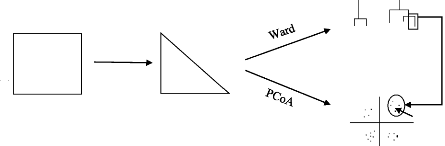
Figure 9: Method used for the ornithological communities analysis: Bray-Curtis = methods used for the creation of the distance matrix, Ward= Ward's minimum variance method used for the cluster analysis, PCoA= Principal Coordinate Analysis used for the ordination analysis, IndVal=Indicator Species Analysis.

Firstly, the data matrix was conversed into a distance matrix through the estimation of the sites «proximity» regarding the observed species and their abundance. It is therefore a multivariate measure of the differences existing between sites.

Among the distance calculation methods, that of Bray-Curtis (D 14) was selected for the analysis on the species communities based on the abundance data. Bray-Curtis index is a distance coefficient calculated from the Steinaus similarity coefficient (S17) that compares two sites (x1, x2) in terms of the minimum abundance of each species. The D14 formula is

where W is the sum of the minimum abundances of the different species, this minimum being defined as the abundance at the site where the species is the rarest. A and B are the sums of the abundances of all species at each of the two sites respectively (LEGENDRE and LEGENDRE, 2012). This index was chosen because it can be used on abundances frequencies and because a same difference between two sites for abundant of rare species has the same contribution to the similarity.

The cluster analysis gives a graphical representation (dendrogram) that was used to determine, from the Bray-Curtis distance matrix, the similar bird communities' compositions among the different sites. It also provided the opportunity to see how the sites rank in comparison to each other.

A hierarchical agglomerative clustering method was used to join together the more similar sites. The term «hierarchical» signifies that the position of a site was definitively imposed within a branch of the classification. The term «agglomerative» refers to the discontinuous partition of the objects where those are considered as being separate from one another. They are successively grouped into larger and larger clusters until a single, all-inclusive cluster is found (LEGENDRE and LEGENDRE, 2012).

The Ward's minimum variance method was chosen (e.g. CONOLE and KIRKPATRICK, 2011; GAILLY, 2013; LOUGBEGNON and CODJIA, 2011) because it aims at finding compact, spherical clusters. To form clusters, this method minimizes the variance across each group as the sites agglomeration progress in minimizing the sum of squared deviation distances from the centroid of each group. Compared to other clustering methods, the Ward's minimum variance method overestimates the distances between sites while the first groups are shaped (LEGENDRE and LEGENDRE, 2012).

The sites similarities calculated from the dendrogram and named cophenetic similarities are different from the original similarities that served to cluster the sites together. Hence, the calculation of the cophenetic correlation allowed us to measure the relationship between the distances of Ward's clustering and the original ones (LEGENDRE and LEGENDRE, 2012).

The Principal Coordinate Analysis (PCoA) allowed us to position the 25 patches, in a space of reduced dimensionality while preserving their distance relationships calculated above as well as possible. The PCoA used the distance matrix calculated before with the goal to find out the axes that maximized that distance matrix (LEGENDRE and LEGENDRE, 2012).

Some distance measures might be negative and did not allow a proper ordination of sites in a full Euclidean space. Therefore, they need a correction for the negative eigenvalues before being used for ordination by PCoA (LEGENDRE and LEGENDRE, 2012).

An indicator species must meet two specific criteria (DUFRÊNE, 2003): it must dominate into a group of sites (specificity index, percentage of individuals in the group) and it must occupy all of the sites within that group (fidelity index, percentage of occupied sites in the group). The IndVal method (DUFRÊNE and LEGENDRE, 1997) was used to identify the species that can be considered as associated to a site or a group of sites. Hence, this method takes into account the specificity and fidelity indices while calculating the species indicator value, giving a percentage proportional to the previous indices. The highest IndVal value obtained identifies the group where the species can be considered as indicator. In addition, the IndVal method allows to test statistically if a species can be considered as being indicator or not.

Moreover, the sum of the species indicator values can be assumed as a criterion in order to compare the clusters formed and choose which one explains the species distribution best (DUFRÊNE and LEGENDRE, 1997).

The following analyses aimed to achieve an investigation of the environmental factors affecting the different patches. It is indeed essential to examine those factors and their distribution within the study area as a first step to interpret the ornithological distribution. We used a multivariate approach using the RStudio(c) software (Version 0.98.976).

To determine the interactions that the environmental variables tended to have with each other in our study area, we performed a principal component analysis (PCA). The PCA is an ordination method that considers the variables altogether and allows the creation of a space of reduced dimensionality from an extraction of the axis that maximize the variance of multidimensional cloud of points shaped by the initial environmental variables. In other words, it condenses the dimension of the cloud of points and helps choose a point of view to look at this cloud of points. The two axes are perpendicular with each other (so they are not redundant) and each one explains

a part of the initial cloud information. Those new descriptors of the information are called principal component and are linear combinations of the initial variables. The roles of those new axes are interpreted while examining the initial variables that are the more correlated (ROBERTS, 2010).

Values of sites characteristics were correlated with the first two principal axes using Pearson and Spearman rank-order correlations coefficients. The reason we used the two methods is that Spearman's correlation coefficient is a non-parametric method unlike Pearson's. Non-parametric methods consist in finding a coefficient correlation, not between the values taken by the two variables, but between ranks of those values. It allows to find out monotone correlations although the variable distributions are skew. The Pearson method only consists of finding the linear relation between values and is easily biased if the two variables don't have a Gaussian distribution or show exceptional values.

The comparison of the two correlation coefficients values brought information about the bias of the correlation calculated. Hence, if Pearson coefficient was higher than the Spearman's one, this means that exceptional values could be present. This would increase the Pearson coefficient value but not modify the more robust Spearman's coefficient values.

IV.4.4. Environmental explicatory factors of the ornithological distribution analysis

For the thesis to be more than descriptive work, an investigation of the influence that the environmental factors have on the bird distribution was realized. The analyses were divided in two sections. The first analysis investigated the influence of the environmental factors on the previously calculated descriptive parameters of the ornithological through multivariate analysis (indirect gradient analysis). Then, Generalized Linear Models (GLM) were realized to demonstrate the relations existing between the environmental variables and our diversity measures. The third analysis directly confronted the bird abundance data matrix with the environmental factors through a multivariate analysis called the redundancy analysis (RDA; direct gradient analysis).

To determine how the ornithological descriptive parameters (species richness, CSI and Shannon index) were affected by site characteristics, the ornithological parameters were correlated with the previous PCA axes using Pearson and Spearman correlation coefficients.

Regressions equations allowed us to formalize the relationship existing between explicative variables and variables to explicate. We used GLMs in order to determine which variables or sets of variables had the largest influence on the overall species richness, Shannon index of heterogeneity and CSI.

For the following analyses, we transformed our previous set of explanatory environmental variables so they approach a normal distribution. A p-value was estimated for each variable through a Shapiro-Wilk test (ROYSTON, 1982) to confirm or not the normal distribution.

All GLM models were constructed in Rstudio(c). We used information-theoretic methods to compare models incorporating different environmental variables, because of the advantages of that method over stepwise approaches for this type of analysis (WHITTINGHAM et al., 2006). To identify the most biologically relevant models, we used the small sample size Akaike's Information Criterion (AICc). We identified the model showing the lowest AICc as the best model (BURNHAM and ANDERSON, 2004; WHITTINGHAM et al., 2006).

Two other criterions were important as well to give information on the model quality. The residual standard error (RSE) that describes the standard deviation of points formed around the linear function, and estimates the accuracy of the dependent variable being measured. And the coefficient of determination (Adjusted-R²) that describes the percentage of the observation variability that is explain by the regression equation.

Relationships between communities and the overall environmental variables were assessed with a canonical ordination method. The RDA is a multivariate analysis method commonly used in ecology in order to analyze simultaneously two data tables (e.g. GAILLY, 2013; SATTLER et al., 2010). It is the multivariate analog of simple linear regressions. The RDA analysis combines the ordination and regression concepts. It allows the ordination of the «species» variables constraints by a canonical axis that is maximally related to a linear combination of the environmental variables (LEGENDRE and LEGENDRE, 2012). It allows the representation at the same time of the species, the patches and the environmental variables in a space of reduced dimensionality.

We used a RDA in this thesis to link the species abundance data set together with the environmental variables. We also projected the Ward clusters obtained previously in the space of reduced dimensionality in order to characterize them.

The 6 respective visits into the 25 patches allowed us to survey 49 bird species. After deletion of the non-breeding visitors (9 species), passage migrants (2 species), presumed escaped birds (4 species) and a resident bird species that was every times recorded as flying over the census area (Hirundo Rustica), 34 species were kept for the analyses (Appendix 2). The following results give an overview of the ornithological descriptive parameters distribution in the 25 patches. The notations for the 3 variables will be as follow: bird_R (bird species richness), SHANB (Shannon index of bird diversity), CSI (community specialization index).

A conservation value was first planned to be calculated for each patch, however it has not been completed since out of all the bird recorded, none of the species were listed as «threatened» or «near threatened» in the «Asian Bird Red Data Book» (BIRDLIFE INTERNATIONAL, 2001).

All of the 34 species can be assumed to be synanthropic species in view of the situation of the study area. Two of the species kept for the analyses were identified as invasive species according to the GLOBAL INVASIVE SPESCIES DATABASE (2005): Columbia Livia (Rock Pigeon) as an alien invasive species and Acridotheres tristis (Common Myna) as a native invasive species. Nevertheless, the number of known alien species in Thailand was still far from being realistically estimated (NAPOMPETH, 2002).

Table 7 shows the species richness distribution within the 25 patches and its completeness while comparing them with the Jack-Knife estimated real richness.

All of the cumulative richness curves tend to an asymptote. Figure 10 shows two distinct curves got for patch No. 8 and patch No. 3. Their Jack-Knife estimated real richness tends to the same number of species (21.5 and 21.3 species respectively), however the two curves show different shapes. Indeed, the surveys in patch No.3 reached faster the real species richness than the surveys carried out in patch No. 8. Hence, at least four surveys were necessary in this case to get reliable data. Concerning the slopes the curves at the last survey, the No. 3 is 0.5 and No. 8 is 0.3. This signifies that in theory to get one new species, 2 supplementary surveys needs to be realized for patch No. 3 and 3 for patch No. 8. The samplings completeness is therefore acceptable.

Another observation made while comparing the species richness results is the time of the day of the survey. After a verification of the normality of the data, a paired t-test of Student was done in order to compare the mean bird richness observed in a park during the morning to the one observed in the afternoon. The test showed that the true difference in means was not equal to 0 (p-value= 8.627x10^-7). Thus, the average species found during the morning surveys appear to be greater than the ones during the afternoon surveys (see Appendix 3 for the entire results).

The Figure 11 below illustrates the previous richness distribution within the study area.

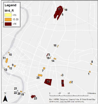
Figure 11: Map of the Species Richness per patch in the study area (bird_R=Bird Species Richness)

Regarding the species distribution, 12 of the 34 species were found in 21 to 25 of the patches surveyed while 11 of them were only found in 1 to 5 patches (Figure 12). Acridotheres grandis (White-vented Myna), Acridotheres tristis (Common Myna) and Copsychus saularis (Oriental Magpie Robin) had the higher range of distribution as they were found in the 25 patches surveyed.

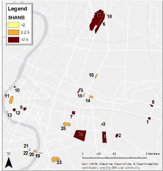
Figure 12: Amount of species characterized by different distribution (number of records) in the study area. Distribution classes: very high (21 to 25 records), high (16 to 20 records), medium (11 to 15 records), low (6 to 10 records) and very low (1 to 5 records)

We generated a map (Figure 13) in order to compare the 25 patches Shannon index of diversity. We found that the patches No.21 and No.22 showed the lowest species diversity while the highest heterogeneity was situated in the patches No.4, No.6 and No.17.

Figure 13: Map of the Shannon Index of Diversity per patch in the study area (SHANB= Shannon index of bird diversity)

Concerning the individuals' relative abundance, it is not surprising that the two species that showed the highest count within the study area appear to be two widespread urban species: Passer montanus (Eurasian Tree Sparrow) and Columba livia (Rock Pigeon). On the other hand, 16 species show a very low abundance (Figure 14).

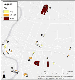
Figure 14: Amount of species individuals characterized by different relative densities (total of the abundance scores) in the study area. Relative abundance classes: very high (101 to 125), high (76 to 100), medium (51 to 75), low (26 to 50) and very low (1 to 25 records)

The species having the highest SSI (species specialization index) are Amaurornis phoenicurus (White-breasted Waterhen), Passer flaveolus (Plain-backed Sparrow)⁷. Conversely, Copsychus saularis (Oriental Magpie Robin), Acridotheres tristis (Common Myna) and Acridotheres grandis (White-breasted Myna) seems to be the more generalist species.

Concerning the CSI (community specialization index) calculated for all the patches, Figure 15 illustrates its distribution within the study area. The highest CSI was found in patch No.17 while the smallest was in patch No.22.

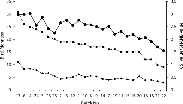
Figure 15: Community specialization Index (CSI) distribution in the study area

⁷ Apus affinis (House swift) was also listed a one of the most specialized species because it has been recorded only once perched in a patch while it was seen often flying over the patches. This species won't be taken into account in further statistical analyses.

In order to bring to a discussion of the previous parameters describing the ornithological data, it will be interesting to compare the evolution of their values in the 25 patches. Therefore, we decided to draw a graph of their evolution on Figure 16. The x-axis of the graph organizes the patches from the highest to the smallest bird species richness observed. We can see that the general decreasing trend is similarly for the three indices with the presence of peaks and troughs more contrasted for the Shannon index.

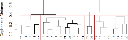
Figure 16: Comparison of the describing parameters of the ornithological data calculated in the 25 patches studied
(bird_R =bird species richness, CSI = community specialization index, SHANB= Shannon index of species diversity)

The Ward's minimum variance method allowed us to classify the sites in different groups on the basis of their species composition. The result of the cluster analysis for the abundance data is illustrated on the dendrogram on Figure 17 below.

Figure 17: Dendrogram formed out of the Ward's minimum variance method from the ornithological abundance dataset.
Four major groups were identified

The cophenetic correlation coefficient calculated for Figure 17 has a value of 0.523.

A clear differentiation was firstly made between group 1-2 and 3-4, showing us the fundamental species abundances distance between the patches of those groups. While comparing those results with the previous SHANB curve (Figure 16: Comparison of the describing parameters of the

ornithological data calculated in the 25 patches studied
(bird_R =bird species richness, CSI = community specialization index, SHANB= Figure 16), we can easily assume that the two first groups contain high species abundances while the groups 3 and 4 show lower abundances. Still, four groups were chosen in order to get more precise indication of the bird abundances distributions. This being said, group 4 separates then 2 patches (21 and 22) showing together similar low abundance trends. 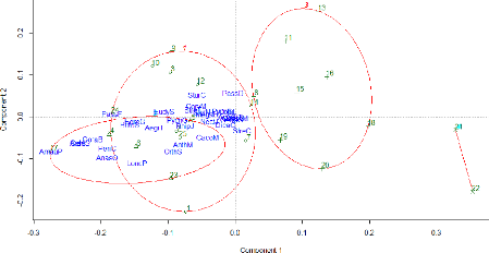On the other side, the cut off between groups 1 and 2 is harder to describe.

The ordination method (PCoA in this case) offered the possibility to illustrate the result of the cluster method in a space of reduced dimensionality where the sites have been localized regarding their species abundance scores (Figure 18).

Figure 18: Factorial design created with the two first axis of the PCoA concerning the abundance data. The red ellipses allow the visualization of the four groups of sites defined earlier by the Ward's method.

The two first axes of the PCoA explain 37.09% of the point variability. The first axis (component 1) explains 24.03 % while the second (component 2) explains 13.05%.The first axis shows well the isolation of groups 3 and 4 from the other groups that are partially overlapping each other. Regarding the avian influence, it is quite hard to visualize bird assemblages at this point.

The IndVal method applied on the abundance data allowed the identification of 11 significant indicator species (p-value < 0.05) separating from each other two groups of sites. All the species listed in Table 8 were selected because they were indicators of the first and second group of sites defined by the Ward clusters (None of the species listed in the two other groups had a significant IndVal value). Some species were not significantly kept from the IndVal analysis due to their lack of specificity or their rarity in the surveys that didn't satisfy the two criterions of the method (i.e. specificity and fidelity).

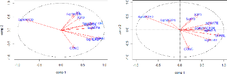
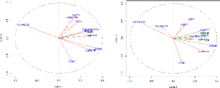
Table 8: Species selected via the IndVal method as being significantly associated to a group of sites

The two groups obtained in the previous table showed various visible differences. First, considering the species record frequencies in the 25 patches, the first group holds widespread synanthropic species while compared with the second one. However, the species of the second group show higher IndVal indices than in the first one.

The correlation matrix (see Appendix 5) showed that a few of the environmental variables (SHANL and nLC; SHANL and WOOD) presented together a correlation coefficient higher than 70% and there was no correlation of the landscape variables with the spatial variables. The landscape richness (nLC) was eliminated from the landscape variables because the information given was poor, while we decided to keep all the others.

By contrast, the spatial variables were for the most part correlated. As their redundancy didn't offer real facilities for the subsequent interpretations, 9 of the 11 variables were deleted. The two left are X³+Y³ and Y³, as together, they were correlated with all of the other spatial variables.

The PCA (principal component analysis) reported the relationships between variables in the research of explanatory factors (for the numerical values see Appendix 6). Before the start of the analysis, the environmental factors have been log or squared-root transformed in order to tend as much as possible to a normal distribution. Hence, the variables AREA, HERB and WATE have been log-transformed while the WCON, SFACTOR, WOOD and Y3 were square root-transformed.

The two first axes of the PCA (PC1 and P) explain respectively 41% and 19% of the total variance of the data set, which means a total of 60%.

As we assume an axis is correlated if |r|>0.60 (Table 9), the axis 1 of the PCA appears positively correlated to SHANL (91%), logAREA (76%), logHERB (74%), SqrtSFACTOR (73%) and logWATE (68%) and negatively correlated to SqrtWOOD (80%) regarding the Pearson correlation coefficients (Figure 19). Concerning their Spearman correlation indices, they are quite close of the previous ones except for the SqrtFACTOR variable that doesn't appear correlated in this case (Figure 19). It is also remarkable that the variable WCON shows here an opposite sign. This is due to the presence of three exceptionally great values that overestimate the Pearson correlation coefficient value.

The landscape heterogeneity appears to parallel the all other factors on the first axis except for the percentage of wooded area and the connectivity of a site (the latter correlation is low). This axis opposes therefore the more open, large sites having a more heterogeneous landscape to the more wooded ones. It is true that within our study area, a bunch of very small patches were wood highly covered while the large patches contained more water and herbaceous cover, meaning more heterogeneous landscapes.

Axis 2 seems to be relatively correlated with the spatial variables (Y3: r =65%) regarding its Pearson coefficient, especially with the longitude which is a direction going from the South to the North. However, the Spearman correlation coefficient is lower than 0.6 because of three exceptional values (three patches being together far more North than the others). Moreover, the percentage of concrete in the sites seems to be negatively correlated to this axis (CONC: r =-66%).

Then, Figure 20 displays the representation of the patches along the two axes with the roles of those new axes interpreted.

Table 9: Pearson and Spearman correlation coefficients between the environmental variables and the two axes of the PCA.
The numbers highlighted show a correlation with the axis

Environmental Factors		PC1		P
Environmental Factors	PEARSON	SPEARMAN	PEARSON	SPEARMAN
logAREA	0.761	0.676	0.081	-0.020
SqrtWCON	0.305	-0.274	0.588	0.353
SqrtSFACTOR	0.731	0.569	0.252	0.061
SqrtWOOD	-0.810	-0.786	0.386	0.475
logHERB	0.735	0.705	-0.341	-0.374
logWATE	0.683	0.731	0.208	0.249
CONC	0.310	0.200	-0.657	-0.690
SHANL	0.914	0.921	-0.302	-0.202
SqrtY3	0.394	0.245	0.650	0.403
X3Y3	0.456	0.409	0.482	0.563

Figure 19: Representation of the environmental variables in the Pearson and Spearman correlation circles formed by the two

The longer the red arrow is, the more variance is explained from the factorial design and the closer the arrow is from an axis, the more it contributes.

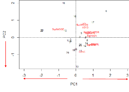
Figure 20: Factorial design created with the two first axis of the PCA concerning the environmental data.

ENVIRONMENTAL FACTORS EXPLAINING THE ORNITHOLOGICAL DISTRIBUTION V.4.1. Indirect gradient analysis

The study of the role played by the environmental factor on the ornithological distribution started with an analysis of the correlation of the ornithological descriptive parameters with the two axes of the previous PCA on the environmental factors.

Figure 21 Representation of the environmental variables (red arrows) together with the ornithological descriptive parameters (green arrows) in the Pearson and Spearman correlation circles formed by the two first axes of the PCA. Only one green arrow represented the three ornithological parameters in the Pearson correlation circle for a better visibility as the three arrows were merged together.

Figure 21 and Table 10 show both the positive correlation of the ornithological description variables with the first axis of the PCA. This means that species richness, Shannon index and CSI, became greater within patches showing larger areas as well as more open and heterogeneous landscapes.

Table 10: Pearson and Spearman correlation coefficients between the ornithological variables and the two axis of the PCA.
The numbers highlighted show a correlation with the specified axis.

For the following analysis, it is important to note that three environmental variables didn't reach a normal distribution (Shapiro-Wilk test: p<0.05): WCON, SHANL and Y3. We kept the same transformation as before for the other environmental variables. Table 11 presents a summary of the GLMs.

Table 11: General linear models and summary statistics for ornithological variables. Predictor environmental variables are patch area (logAREA, log-transformed), weighted connectivity (SqrtWCON, Square root-transformed), S-Factor (SqrtSFACTOR, Square root-transformed), Wood cover (SqrtWOOD, Square root-transformed), Herbaceous cover (logHERB, log-transformed), Water cover (logWATE, log-transformed), Concrete cover (CONC), Y³ (SqrtY3, Squared root transformed), X³+Y³(X3Y3). a= first parameter, b= second parameter (environmental factor coefficient), R²= coefficient of determination, RSE= Residual Standard Error, AICc = Akaike's information criterion corrected for small sample size. The best models are indicated in bold for each ornithological variable.

	~logAREA	-13.612	2.993	0.721	2.692	125.524
	~SHANL	8.531	10.176	0.467	3.720	141.691
	~logWATE	13.536	2.866	0.428	3.855	143.475
	~SqrtSFACTOR	-8.423	22.996	0.323	4.191	147.656
	~logHERB	13.484	2.126	0.236	4.453	150.683
bird_R
	~SqrtWOOD	28.371	-1.456	0.168	4.648	152.827
	~X3Y3	-2,087.000	2,066.000	0.098	4.840	154.849
	~SqrtY3	-507.424	10.305	0.058	4.946	155.934
	~CONC	18.208	-6.208	0.019	5.047	156.949
	~SqrtWCON	17.443	15.060	-0.017	5.138	157.836
	~SHANL	1.618	0.866	0.594	0.247	6.176
	~logWATE	2.062	0.232	0.490	0.277	11.861
	~logAREA	0.542	0.178	0.423	0.295	14.964
	~SqrtSFACTOR	0.471	1.699	0.302	0.324	19.722
	~SqrtWOOD	3.376	-0.134	0.263	0.333	21.062
SHANB
	~logHERB	2.091	0.157	0.218	0.343	22.545
	~X3Y3	-201.200	0.000	0.184	0.351	23.608
	~SqrtWCON	0.929	-0.054	-0.043	0.358	24.598
	~SqrtY3	-34.474	0.723	0.042	0.380	27.611
	~CONC	2.435	-0.366	-0.006	0.389	28.853
	~logAREA	-0.598	0.108	0.693	0.104	-37.202
	~logWATE	0.395	0.095	0.342	0.152	-18.141
	~SHANL	0.251	0.315	0.317	0.155	-17.225
	~SqrtSFACTOR	-0.271	0.709	0.214	0.166	-13.717
	~logHERB	0.396	0.070	0.178	0.170	-12.582
CSI
	~SqrtWOOD	0.925	-0.054	0.167	0.171	-12.256
	~SqrtY3	-20.240	0.408	0.073	0.181	-9.595
	~X3Y3	-69.200	0.000	0.071	0.181	-9.531
	~SqrtWCON	0.521	0.617	-0.011	0.189	-7.430
	~CONC	0.565	0.000	-0.038	0.191	-6.757

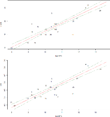
Considering concrete cover, weighted connectivity or the two spatial variables as predictors for the three ornithological variables respectively, provided the lowest relative statistical evidence and explanatory power.

Species richness and CSI increased with the patch area while Shannon's index Bird diversity increased with the water cover rate (Figure 22 and Figure 23).

Figure 22: Residuals plots of best GLM: bird species richness (top row) and log-transformed CSI (bottom row) as a function of the patches log-transformed area

Some of the patches deviate from the regression line in both plots (Figure 22). Patches No. 3, 5, 6, 10 and 19 showed higher bird richness while patches No. 7, 11, 18, 20 and 24 contain lower bird species than the regression line. Those trends need an interpretation regarding the factors affecting the deviation of the patches in comparison with the ones situated along the regression line (patches No. 15, 21, 6,1 for example). The same was completed with the CSI plot.

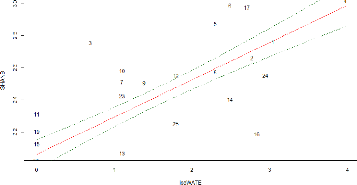
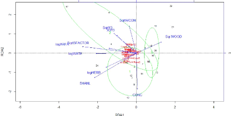
Figure 23: Residuals plots of best GLM: Shannon index of bird diversity as a function the patches log-transformed water cover.

In this case, the patches are more scattered. The patches No. 3 and 16 show both the higher deviance from the regression line, the first one showing a higher Shannon index of bird diversity and the second showing a lower one.

Finally, a redundancy analysis (RDA) was realized with the ornithological data (abundance matrix) and the environmental factors in order to identify the relationships between the two data sets.

As we have 10 environmental variables, we have 10 constrained ordination axes (RDA 1 to RDA 10). In total, the variance explained by the constrained axes (independent variables, i.e. environmental variables) is equal to 53% while the rest (47%) is explained by the unconstrained axis (dependent variables, i.e. bird abundance).

We will focus on the two first axes of the RDA (Figure 24) that show the highest variance explained in order to simplify the interpretation. The red names represent each individual species displayed in the RDA space and the blue vectors show how the environmental variables fall along that RDA space. The longest vectors along each RDA axis are the most influent in explaining variation of species abundance along that axis.

The first two constraints axes of the RDA explain respectively 37% and 16 % of the common variance among species and environmental factors (a total of 53% explained). While those two axes explain respectively 9% and 8% of the species abundance variance (17% in total). The plot (Figure 24) doesn't allow us to visualize the actual species impacts on the patches distribution between the two RDA axes. Regarding the environmental variables, three variables are negatively correlated (|r|>0.60) with the first axis of the RDA: logAREA, logWATE and SHANL (Table 12).

Figure 24: Representation of the species abundance and environmental variables in the plot formed by the two first axes of the RDA. The green ellipses show the Ward clusters obtained previously. An ellipse contains 80% of the patches of a group.

The four previous clusters obtained at section IV.4.2 via the Ward minimum variance method can be visualized on the factorial design shaped by the two first axes of the RDA (Figure 24). That allows their characterization. Group 1 and 2 are thus characterized by more open (more herbaceous and concrete cover), heterogeneous landscapes while group 3 and 4 seem characterized by a more wooded context. Group 2 is elongated by the spatial variables, situating those patches more in the North of the study area. They are also characterized by large patches with water.

Table 12: Pearson and Spearman correlation coefficients between the environmental variables and the two axes of the RDA.
The numbers highlighted show a correlation with the specified axis.

Environmental Factor		PC1		P
Environmental Factor	PEARSON	SPEARMAN	PEARSON	SPEARMAN
logAREA	-0.858	-0.759	0.101	0.018
SqrtWCON	-0.115	0.124	0.426	0.165
SqrtSFACTOR	-0.439	-0.362	0.076	0.160
SqrtWOOD	0.401	0.417	0.174	0.105
logHERB	-0.487	-0.465	-0.219	-0.158
logWATE	-0.642	-0.637	-0.005	-0.158
CONC	0.016	-0.036	-0.560	-0.540
SHANL	-0.669	-0.677	-0.382	-0.139
SqrtY3	-0.360	-0.136	0.312	0.077
X3Y3	-0.312	-0.262	0.278	0.365

Over the century, as urbanization growth accelerates, urban green areas are facing severe recession. As the urban sprawl is continually extending due to land speculation and uncontrolled development, wildlife and people are getting closer and closer and the conservation of urban biodiversity emerges as a concern of rising importance (MCKINNEY, 2002).

The potential impact of urbanization on the avifauna has been largely studied worldwide. However, although Bangkok is a booming megacity where the environment has been severely damaged, there has not been any previous studies focusing on the overall urban bird species distribution (ROUND, 2008). Therefore, this thesis was the timely opportunity to report the situation of the birds in Central Bangkok so there can be basis implemented for a future monitoring.

We will guide the discussion through the answers to the two research questions, namely:

- How is the avifauna characterized and distributed into green patches situated in the center of the Bangkok Metropolis?

- How do the environmental parameters of those green patches influence the bird distribution?

In order to best inform the wildlife conservation strategies, a section regarding the conservation implications will then be highlighted. Finally, some result need to be nuanced and a section will focus on the limitations of this study.

HOW IS THE AVIFAUNA CHARACTERIZED AND DISTRIBUTED INTO GREEN PATCHES SITUATED IN THE CENTER OF THE BANGKOK METROPOLIS?

The results obtained through the ornithological distribution analysis bring a descriptive overlook of Bangkok's avifauna distribution. Those results will be discussed together with the literature review statements in order to be correctly replaced in the thesis context.

Firstly, the bird species sampled (49 species) represented 13 % of the birds assumed to be in the region of the Bangkok Metropolis all year round (LEPAGE, 2014). This is a quite poor amount but it was predictable as we focused our study area in the most urbanized part of the city. It confirmed the statements made by many previous studies, suggesting that species richness decreases as urban development increases (CHACE and WALSH, 2006; DEVICTOR et al., 2008; IMAI and NAKASHIZUKA, 2010; MCKINNEY, 2006; NIELSEN et al., 2013; ORTEGA-ÁLVAREZ and MACGREGOR-FORS, 2009; SANDSTRÖM et al., 2006).

A great part of the bird species found in the green patches sampled were common native synanthropic species in the Bangkok region like previously pointed out by ROUND (2008). A great part of those species were found in the first indicator species group (Table 8), those species being widespread, often abundant and easily detectable. Those common native species are of great importance for conservation purpose, since their presence contributes to the structure, biomass and energy turnover of the environment they live in (GASTON, 2010). It is all the more important as those species remain frequent victims of habitat loss as well as species invasion and this can have deep impacts on their environment and the ecosystem services they provide. Indeed, the interactions between those common species with city dwellers can influence positively their wellbeing and increase their relation with nature (MILLER and HOBBS, 2002). The latter argument is essential because it brings a socio-economic motivation for the Bangkok administration to invest in the support of avian biodiversity.

The species abundance structure (Figure 14) showed that most of the urban species recorded are non-abundant while only a few are very abundant. Indeed, some species are able to find alternative ecological niches in the cities and develop quite significant populations alike the common native synanthropic species listed before. However, those adaptions were also made by few well known urban-exploiter bird species (native or alien) that created excessive populations like Columbia Livia (Rock Pigeon, alien) and Acridotheres tristis (Common Myna, native) pointed out as invasive species in the GLOBAL INVASIVE SPECIES DATABASE (2005). Today's issue is that those abundant species tend to become overabundant and create competition with other native birds, forcing the decreasing of the latter's abundance (CONOLE and KIRKPATRICK, 2011; DEVICTOR et al., 2008; MCKINNEY, 2006). It is nevertheless important to nuance the statement that stipulates that a species is invasive at the whole study area scale. Indeed, even if some species were more widespread and abundant than others across the whole study area, it would be essential to look at the invasiveness problem at the patch scale and explore the metapopulation dynamics (ANDERIES et al., 2007).

The PCoA ordination axes (Figure 18) don't explain a high part of the variance between the patches regarding their bird assemblages based on the species abundance. External factors could better explain the bird abundance distribution within the study area. Indeed, neutral mechanisms like biotic processes such as scattering or competition, may play a subordinate role in structuring community composition in urban spaces. According to SATTLER et al. (2010), human disturbance happening in this case on a regular and frequent basis by the multiple human activities could cause inhibitions of both the development and installation of spatially organized biotic processes. Environmental parameters may play a role as well and their case is discussed below.

HOW DO THE ENVIRONMENTAL PARAMETERS OF THOSE GREEN PATCHES INFLUENCE THE BIRD DISTRIBUTION?

In order to go further than an assessment of the effect of urbanization on birds through the creation of species lists and to best inform wildlife-conservation strategies, it is crucial to understand the ornithological responses to the modified environmental features of Bangkok.

We know that Bangkok urban green patches are essential to provide habitat for birds (ROUND, 2008). It is true that the use of a habitat by a bird differs between every species as well as in between the same species (FULLER, 2012). However, for conservation purposes, it is important to attribute the species found in each patch to the way they use their environment through the evaluation of the observed differences in overall species abundances. The environmental features investigated in the urban green patches of central Bangkok supported various bird assemblages that may in part reflect the availability of different resources. For example, green patches with more water were more inclined to host bird characteristics of wetlands. Nevertheless, analyses of community-wide indices are complex to interpret because they contain a composite response of many individual bird species (PEARSON, 1993).

The previous tests realized through section V.4 showed that in the context of Central Bangkok, the size of the patches had the highest influence on bird species richness and CSI (Figure 22 and Table 11). This doesn't follow statements made by previous researchers in other regions, which demonstrated that green patches' internal habitat qualities are of greater importance than both park size and park isolation for the bird richness and composition (NIELSEN et al., 2013). We explained the patches showing higher species richness (or CSI) than the regression line (Figure 22) as being more heterogeneous patches. The ones below the line, especially patch No. 11 (Sanam Luang Park) are assumed as being more homogeneous, in this case with a high herbaceous cover rate.

The bird species heterogeneity (SHANB), on the other hand (Figure 23), was the most influenced by the rate of water cover in the patches. In this case, the patches below the regression lines seemed to be homogeneous but with high wooded cover rates in the case of patch 16, therefore, the detection of the birds is assumed as poorer than in other patches.

The following paragraphs study separately the environmental variables types regarding their influence on the ornithological dataset.

As suggested by other studies as well as by the IBT ( e.g. CASTELLETTA. et al., 2005; FERNÁNDEZ-JURICIC and JOKIMÄKI, 2001; MACARTHUR and WILSON, 1963, 1967, NIELSEN et al., 2013), a biogeographic variable, the area of the patches, was the environmental variable affecting the bird richness the most (Figure 22 and Table 11). The area of the patches was also

of greatest influence on the bird diversity estimated with the Shannon index of heterogeneity that takes into account abundance of each species recorded at one site. Bird communities at a site contained also more specialized species in larger area patches. The isolation index didn't show evident influence on the ornithological variables, contrary to what has previously been predicted by the IBT (MACARTHUR and WILSON, 1963, 1967, NIELSEN et al., 2013). The possible causes will be later discussed in section VI.3.3.

A first landscape factor explaining highly the bird diversity was the rate of water cover. It tended to bring more species to the patches including more wetland specialized species alike Anastomus oscitans (Asian Openbill), Egretta garzetta (Little Egret), Ardeola sp. (Pond Heron), Butorides striata (Little heron), or else ,Amaurornis phoenicurus (White-Breasted Waterhen).

Surprisingly, we found a negative influence of the percentage of wooded cover on the bird species diversity that doesn't corroborates some previous studies that found that trees play an important role in explaining urban bird diversity (e.g. EVANS et al., 2009; SANDSTRÖM et al., 2006; SATTLER et al., 2010). Two reasons can explain those trends; first, the detectability of birds decreased with an augmentation of wood cover and second, the larger patches of our study areas were mostly composed of heterogenetic landscapes while the smaller patches contained merely wood cover.

More herbaceous cover, which was highly correlated with the Shannon index of landscape heterogeneity seemed to have greater influence on the more synanthropic group of species (group 1). The concrete cover showed the same trends but has less influence.

Finally, even if environmental variables accounted for a large percentage of the explanatory power of the bird community models, an important part of the bird community composition seemed to be determined by environmental stochasticity, i.e. «random events such as habitat destruction by human activity, anthropogenic transportation or the introduction of exotic species» (SATTLER et al., 2010). Environmental variables can explain some variation in urban bird community composition, however, stochasticity, appeared to be more important in urban areas than in other habitat types, where avian species communities are far from stable, enduring constant change while adapting themselves to the disturbances and changes that constantly modify their habitat (SATTLER et al., 2010).

As the results obtained before are discussed, it is important to have a critical subsequent approach on the data quality and directions taken through the overall thesis.

A study of the birds in central Bangkok (Thailand) in order to implement the basis of a long term monitoring

IV. METHODOLOGY