3.3.3.2. Analysis of the determinants of communities'
vulnerability to flood
1) Analysis of Flood Characteristics
a) Flood frequency and magnitude
analysis
The magnitude of an extreme event is inversely related to its
frequency of occurrence, very severe events occurring less frequently than more
moderate events (Maiti, 2007, p 44). The objective of frequency of occurrence
is obtained through the use of probability distributions. Some of the commonly used probability distributions
are: Gumbel's or Extreme Value type 1 distribution (EV1); Log-Normal
distribution; Log-Pearson type III distribution (LP3), and Method of plotting
position.
For this study, further insight into flood frequency is provided
by the return period analysis. The return period was obtained using the most
efficient formula for computing plotting positions for unspecified
distributions and now commonly used for most sample data: the Weibull equation
(1). The objective of the method is to build the relation between the
probability of the occurrence (return period) of a certain event and its
magnitude. Frequency is how often an event of a given magnitude may be expected
to occur in the log-run average.
The annual peak discharge data of the Mono River at Athieme
station (1971-2010, N= 40 years) is selected for flood frequency analysis. A
simple technique was to arrange the given peak in descending order of magnitude
and assigned an order number (m). The probability of occurrence for each observation is
given by:
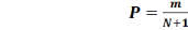  (1) (Sreyasi Maiti 2007, p 45) (1) (Sreyasi Maiti 2007, p 45)
Where: P= Probability of occurrence; m= order number of the
event; N= Total number of events in the data; The return period for each
observation was determined using the following formula:
  (2) (Sreyasi Maiti 2007, p 45) (2) (Sreyasi Maiti 2007, p 45)
Where: T = return period (Recurrence interval or frequency)
Depending on the flood peaks recorded in 2010 for the study area
and the average flood peaks for the examined period, floods are classified
according to their magnitude.
b) Flood duration and flood water level
assessment
Data on flood duration and flood water levels were obtained from
each household from interview. The interviewed household could recall the peak
duration of flooding during the latest more severe flood (2010). The average
days recorded from household interviews was calculated for each village. Flood
water levels were measured inside the house as revealed by marks on building
walls with reference to the ground floor during the interviews. Only houses in
the main village (populated area) were considered. The flood water levels were
ranged from the lowest level to the highest level for each village.
3.3.3.3 Analysis of
human-environmental condition
Statistical analyses were used as the methods for
human-environmental condition components analysis. It includes descriptive
statistics to describe all the data in general.
3.3.3.4 Computation of
Flood Vulnerability Index (FVI)
The collected data were arranged in the form of a
rectangular matrix with rows representing villages and columns representing
indicators. In order to obtain figures which are free from the units and also
to standardize their values, the indicators were normalized so that they all
lie between 0 and 1. After computing the normalized scores the index is
constructed by giving unequal weights to all indicators.
1) Normalisation of
Indicators Using Functional Relationship
Two types of functional relationships are possible:
vulnerability increases with increase (decrease) in the value of the
indicator. The study used then two formula to normalise indicator, depending on
their functional relationship with vulnerability. Then, in case that the
indicator has an increase functional relationship with vulnerability (positive
indicators), the normalisation is done using the following formula:
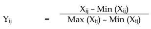
(3)
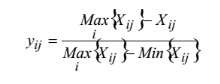
On the other hand, in case that the indicator has a decrease
functional relationship with vulnerability (negative indicators), the
normalized score is computed using the formula:
(4)
Xij denotes the value of j indicator (j=1, 2, .........30) in the
i village (i=1, 2-, ....8).
Yij is the matrix corresponding to the normalised score;
Wj and Yij lie between 0 and 1; Ó Wi = 1
It is obvious that the scaled values of Yij lies between 0 and
1. The value 1 corresponds to that village with maximum value and 0
corresponds to the village with minimum value. Through those formula the
normalised scores for each indicator were obtained using MS-EXCEL Max() and
Min() functions.
2) Method of Weighting
and Aggregation of Indicators into Vulnerability Index
After computing the normalized scores, the index is
constructed by giving an unequal weight to all indicators. In literature,
several methods are used to give weight to indicators either equal weights
(simple average of the scores and Patnaik and Narain Methods) or unequal
weights (Expert judgement and Iyengar and Sudarshan's methods) or multivariate
statistical techniques (Principal components and cluster analysis method).
The present study uses an unequal method of Iyengar
and Sudarshan's to give weight to all indicators. Iyengar and Sudarshan (1982)
developed a method to work out a composite index from multivariate data and it
was used to rank the districts in terms of their economic performance. This
methodology is statistically sound and equally suited for the development of
composite index of vulnerability to climate change. In Iyengar and Sudarshan's
method, the weights are assumed to vary inversely as the variance over the
regions in the respective indicators of vulnerability.
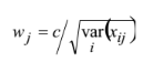
That is, the weight wj is determined by:
(5)
where c is a normalizing constant: equation 6
(6)
The choice of the weights in this manner would ensure that large
variation in any one of the indicators would not unduly dominate the
contribution of the rest of the indicators and distort inter regional
comparisons. It is well known that, in statistical comparisons, it is more
efficient to compare two or more means after equalizing their variances.
The overall village index, Yi , also varies from zero
(0) to one (1) with 1 indicating maximum vulnerability and 0 indicating no
vulnerability at all. the higher the district index, the more the level of
vulnerability .
The composite indicator for flood vulnerability factors
(exposure, susceptibility and resilience) for the ith village was
obtained as:
Yi= ?Wj Yij
(7)
where: Yi is the composite indicator of ith village;
Wj is the weight for each indicator lies between 0 and 1; ?Wj= 1; and Yij is
the normalised scores of indicators.
To ensure that the indices calculated for each vulnerability
factor can be compared, the sum for each factor of exposure, susceptibility and
resilience are divided by their respective number of indicators that describe
each vulnerability factor. The composite vulnerability index for exposure
factor is given as:
  (8) (8)
Where:   is the composite vulnerability index of exposure factor, is the composite vulnerability index of exposure factor,
Wj is the weight a single indicator, ei is exposure indicators;
Yij is the normalised value of exposure indicator; n is the number of
indicators.
Susceptibility and resilience factors can all be represented in
similar way.
Any flood vulnerability analysis requires information regarding
these factors, which can be specified in terms of exposure indicators,
sensitivity indicators and resilience indicators. Finally, the vulnerability of
a system to flood events can be expressed with the following general equation
(Balica, 2007, p 37). This equation is used in the present study to compute
Flood Vulnerability Index (FVI).
Vulnerability = Exposure + Susceptibility -
Resilience (9)
3.3.3.5. Flood vulnerability maps
The composite index values of the three factors
of vulnerability and total flood vulnerability index values were integrated in
ArcGIS 10.1 software with all relevant input data being available in a digital
spatial database (polygon shape file) to produce exposure, susceptibility,
resilience and vulnerability maps. The maps were classified and colour coded
green-yellow-red, indicating low-moderate-high areas, respectively.
| 

