|
NATIONAL UNIVERSITY OF RWANDA
FACULTY OF APPLIED SCIENCES
ELECTRICAL AND ELECTRONIC ENGINEERING
DEPARTMENT
STUDY OF SMART ANTENNAS ON MOBILE
COMMUNICATION
A project report submitted to obtain a BSc degree in
Electrical and Electronic Engineering/Ingénieur en Electricité et
Electronique.
Presented by BUGINGO Philippe
and
NDAMUKUNDA Ismaël
Supervisor: Dr. Felix K. AKORLI
Butare, January 2006
To our parents, brothers and sisters,
To our friends,
This project is dedicated.
ACKNOWLEDGEMENTS
We would like to express our sincere gratitude to our
supervisor, Dr Felix AKORLI, for his invaluable support and
guidance throughout the duration of the research.
We appreciate the tremendous support provide from our parents,
brothers and sisters for their love and encouragement. We would not complete
our degrees without their continuous and immeasurable support.
We would like to acknowledge the support of several students
and staffs at National University of Rwanda; especially, we thank our
colleagues for their collaboration during our studies.
We also would like to thank the following people: Muragijimana
Emmanuel's family, Pastor Munezero's Family, Ntampaka Justin's family,
Ir.Nzamutuma Ismaël, Mr. Ndalibumbye Fidèle, Mr.Harerimana
Emmanuel, Pastor Nahayo David's family, Jyanumucyo choir, Mr. Semana Edmond,
Miss Nyiranteziryayo Grace and her family, Miss Icyimpaye Joyce and her sister
and others who helped us through the years of our studies in National
University of Rwanda.
Last but not the least to Miss Mutezinka Gloriose we
acknowledged her invaluable love and encouragement.
BUGINGO Philippe NDAMUKUNDA Ismaël
ABSTRACT
The purpose of this project is to carry out a study into the
use of smart antennae by mobile communication systems. An introduction which
gives an overview of the project is given. Two methods of antenna synthesis
known as the Woodward-Lawson and Dolph Chebyshev are
presented, of these methods Dolph Chebyshev was used in our design due to its
fast convegence. Antenna theory is discussed with emphasis on array antennas.
With a basic understanding on antenna, this project therefore discusses the
smart antenna by on mobile communication technology. The two types of smart
antenna design approaches known as the Switching-Beam Array and
Adaptive Array are addressed.In the design the Adaptive Array has been considered
since it has the advantage of high capacity property over the Switching Beam
Array. System aspect for a smart antenna technology is also given. After a
brief introduction to the types of multiple access schemes, array antennas
simulation and synthesis using the above mentioned methods is carried out by
varying different limiting parameters. Antenna radiation patterns are plotted
and discussed. It concludes that smart antennas systems are to be deployed in
mobile communication especially in heavily populated area where the number of
subscribers is large.
RESUME
Le but de ce projet est d'étudier la possibilité
d'utilisation d'antennes intelligentes par des systèmes de communication
mobiles. Une introduction qui contient une vue d'ensemble du projet est
donnée. Deux méthodes de synthèse d'antenne connue comme
Woodward-Lawson et Dolph Chebyshev sont
présentées, de ces methodes celle de Chebyshev a
été utilisé utilisée dans notre conception comme
elle est plus convergente. La théorie sur les antennes est
discutée en mettant l'accent sur les systèmes d'antennes.Avec une
compréhension de base sur les antennes, ce projet discute donc de la
technologie d'antenne intelligente sur la communication mobile. Les deux
approches d'antennes intelligentes connues comme Antennes à
commutation de faisceaux et antennes adaptives sont
adressés. Dans la conception, nous avons considéré les
antennes adaptives puisqu'elles offrent une plus grande capacité.
L'aspect d'un système d'antennes intelligentes est aussi donné.
Après une brève introduction aux différentes types
d'accès multiples, la simulation et la synthèse d' un
système d'antennes utilisant les méthodes ci haut
mentionnées sont effectuées, et cela, en variant des
paramètres de limitation différents. Les modèles de
radiation d'antenne sont tracés pour la discussion. La conclusion montre
que le systeme d'antennes intelligentes est recommandable pour être
utilisé dans les régions surpeuplées où le nombre
d'abonnées est très important.
CONTENTS
DEDICACE
Error! Bookmark not
defined.
ACKNOWLEDGEMENTS
ii
ABSTRACT
iii
RESUME
iv
CONTENTS
v
List of Figures
vii
List of Tables
viii
List of Abbreviations
ix
INTRODUCTION
1
CHAP 1 TOWARD SMART ANTENNA
3
1.1 Antenna synthesis
3
1.1.1 Woodward-Lawson Method
4
1.1.2 Dolph-Chebyshev Method
6
1.2 Evolution from Omni directional to
Smart Antennas
8
1.2.1 Omni directional Antennas
9
1.2.2 Directional Antennas and Sectorized Systems
10
1.2.3 Smart antenna
11
1.2.3.1 Switching-Beam Array (SBA)
12
1.2.3.2 Adaptive Array
13
CHAP 2 SYSTEM ASPECTS OF
SMART ANTENNA
16
2.1 Key characteristics of smart
antennas Technology
16
2.2 Signal Propagation: Multipath and
cochannel Interference
17
2.2.1 Multipath and problem associated with it.
17
2.2.2 Cochannel Interference
19
2.3 Difference between uplink and
downlink
20
2.3.1 Uplink Processing
20
2.3.2 Downlink Processing
21
2.4 Handling of common channels
21
CHAP 3 ANTENNA ARRAYS AND BEAM FORMING
23
3.1 Antenna Arrays
23
3.1.1 Introduction
23
3.1.2 Theoretical model for an antenna array
24
3.1.2.1 Linear array antenna
24
3.1.2.2 Planar array antenna
25
3.1.3. Elements spacing
28
3.1.4. Microstrip patch antennas design
29
3.2. Beam forming
30
3.2.1. Nulling Beam Forming
31
3.2.2. Steering Vector
31
3.2.3. Recursive Least Squares Algorithm
32
CHAP 4 Multiple Access
Schemes
34
4.1 Introduction
34
4.2 Frequency Division Multiple Access
(FDMA)
34
4.3 Time Division Multiple Access (TDMA)
35
4.4 Code Division Multiple Access (CDMA)
35
4.4 Space Division Multiple Access
(SDMA)
36
CHAP 5 SIMULATION USING
MATLAB
37
5.1 Analysis and Simulation on array
antenna
37
5.1.1 Variation of number of elements N
37
5.1.2 Variation of Side Lobe Level
39
5.1.3 Variation of Inter-element Spacing.
41
5.2 Discussion
44
CONCLUSION AND RECOMMANDATIONS.
45
References
46
APPENDIX
49
List of
Figures
Fig.1.1 Omni directional Antennas and coverage patterns
[7].
9
Fig 1.2: Sectorized antenna system and coverage pattern
[10].
10
Fig 1. 3: Concept of smart antenna systems [8].
11
Fig 1.4 Switch-Beam Systems [11].
12
Fig 1.5: A Switch-Beam network [11].
13
Fig 1.6: An adaptive antenna [11].
14
Fig 1.7: Network structure of an adaptive array [11].
15
Fig 2.1: The effect of Multipath on a mobile user[8].
17
Fig 2.2: Two out-of-Phase Multipath Signal [8].
18
Fig 2.3:.Representation of Fade Effect on User Signal
[8].
18
Fig 2.4: Illustration of Phase Cancellation [8].
19
Fig 2.5: Illustration of Co channel Interference in a Typical
Cellular Grid [8].
20
Fig 3.1: Linear array of micro strip [5].
24
Fig 3.2: Linear and Planar geometries [6].
26
Fig 4.1: Concept of FDMI system
35
Fig 4.2: Concept of TDMA system
35
Fig 4.3: Concept of a CDMA system
36
Fig 4.4 Concept of SDMA system
36
Fig 5.1 : Radiation pattern with 4 elements
37
Fig 5.2 Radiation pattern with 8 elements
38
Fig 5.3 : Radiation pattern with 10 elements
38
Fig 5.4: Radiation pattern with 5dB.
39
Fig 5.5: Radiation pattern with 15dB
39
Fig 5.6: Radiation pattern with 37dB
40
Fig 5.7: Radiation pattern with 40dB
40
Fig 5.8 Radiation Pattern with normalized inter-element spacing
of 0.125
41
Fig 5.9: Radiation Pattern with normalized inter-element spacing
of 0.5
41
Fig 5.10: Radiation Pattern with normalized inter- element
spacing of 0.75
42
Fig 5.11 Radiation Pattern with normalized inter-element spacing
of 1
42
List of Tables
Table 1 :Results of varying number of elements
38
Table 2: Results of varying side lobe level
40
Table 3 : Results of varying inter-element spacing
43
List of Abbreviations
MATLAB: Matrix Laboratory
GSM:Global System for Mobile Communications (Ex Groupe
Spéciale Mobile).
RF: Radio Frequency
BER: Bit Error Rate
EM: Electromagnetic
DSP: Digital Signal Processor
SBA: Switching Beam Array
TBA: Tracking Beam Array
CDMA: Code Division Multiple Access
SDMA: Space Division Multiple Access
TDMA: Time Division Multiple Access
FDMA: Frequency Division Multiple Access
TDD: Time Division Duplex
FDD: Frequency Division Duplex
AF: Array Factor
RLS: Recursive Least Square
LMS: Least Mean Square
DOAs: Directions of Arrival
INTRODUCTION
It is foreseen that in the future an enormous increase in
traffic will be experienced for mobile and personal communications systems.
This is due both to an increased number of users as well as new high bit rate
data services being introduced. The increase in traffic will put a demand on
both manufacturers and operators to provide high capacity systems in
the networks.
Presently, the only mobile communication campany in Rwanda is
MTN Rwandacell. This company uses either omnidirectional in the sparsely
populated areas or sectorized antennas in the densely populated areas - in the
cities at its base stations. The basic challenge in wireless communication
being the finite spectrum or bandwidth, the only technology believed to be the
latest major technological innovation that has the capability of containing
large increase in mobile communication systems access [1] is the smart
antenna.
Therefore, the aim of this project is to analyse and study
smart antenna system, but also how the system can increase capacity in mobile
communications. Our project is limited to an examination of the design of a
smart antenna system for the base station for mobile communication. We show
that the smart antennas can be implemented at the base station site, without
requiring any changes neither at adjacent base stations nor in the mobile
stations. Cost estimation of design is not included in this project.
The project begins with antennas analysis and discusses the
evolution from omni directional to smart antennas.
Smart antenna system is presented in the second chapter in
which keys benefits, signal propagation, uplink and downlink processing, and
handling of common channel are also discussed.
The third chapter consists of antenna array and beam forming.
Multiple access schemes are discussed in chapter four. This is followed by the
analysis and simulation on array antenna in chapter five and finally the
conclusion and recommendations are given.
CHAP 1 TOWARD SMART ANTENNA
1.1 Antenna
synthesis
In the business and industries worldwide, communications has
become the key to momentous changes as they themselves adjust to the shift
toward an information economy. Antennas provide mother earth a solution to a
mobile communication system.
In [2] it is reported that the antenna is a means of coupling
electromagnetic energy from a transmission line into free space, thus allowing
a transmitter to radiate, and a receiver to receive the incoming
electromagnetic power. It is a passive device and therefore, the power radiated
by a transmitting antenna cannot be greater than the power entering to the
transmitter.
In addition to transmitting and receiving energy, an antenna
in an advance mobile system is generally required to optimize or accentuate the
radiation energy in a particular direction while suppressing it in others.
Physical size may vary greatly and antennas can be just a lens, an aperture, a
patch, an assembly of elements (array), a reflector, or even a piece of
conducting wire [3]. The antenna is one of the most critical elements for
mobile communication systems and a good design of the antenna can ease system
requirements and improve overall system performance.
Practically, it is often necessary to design an antenna system
that produce desired radiation characteristics. In general, there are common
demands to design antenna whose far-field pattern posses nulls in certain
directions or to yield pattern that exhibit a desired distribution, narrow
beamwidth and low side lobes, decaying minor lobes, and so forth.
Hence, antenna synthesis is an approach that uses a systematic
method or combination of methods to arrive at an antenna configuration which
yields a pattern that is either exactly or approximately the same to the
initial specified pattern, while satisfying other system constrains.
From [4], antenna pattern synthesis can be classified into
three categories. The first group that normally utilizes the Schelkunoff
Method requires the antenna patterns to possess nulls in certain desired
direction. The next category, which requires the patterns to exhibit a desired
distribution in the entire visible region, is referred to beam shaping. It can
be achieved by using the Fourier Transform and Woodward-Lawson
Methods.
Finally, the Binomial Technique and
Dolph-Chebyshev Method are usually used to produce radiation patterns
with narrow beamwidth and low side lobes. However, only the Woodward-Lawson
method and the Dolph-Chebyshev method are discussed.
1.1.1 Woodward-Lawson Method
A popular antenna pattern synthesis method was introduced by
Woodward and Lawson. The synthesis is accomplished by sampling the desire
pattern at various discrete locations. Each pattern sample is associated with a
harmonic current of uniform amplitude distribution and uniform progressive
phase, whose corresponding field is known as a composing function.
Each composing function for a linear array is as shown in (1.1)
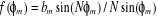 (1.1)
(1.1)
N - Number of elements
bm - excitation coefficient
Öm - Phase excitation
The excitation coefficient bm of every harmonic
current is such that its field strength is
similar to the amplitude of the desired pattern at its
corresponding sampled point. The total excitation of the source is comprised of
a finite summation of space harmonic, and
the corresponding synthesized pattern is represented by a
finite summation of composing functions with each term representing the field
of a current harmonic with uniform amplitude distribution and uniform
progressive phase [5].
The overall pattern produced by this method is described as
follows. The first composing
function yields a pattern whose main beam position is decided
by the value of its uniform progressive phase with the innermost side lobes
level approximately -13.5dB,and while the rest of the side lobes decreases
monotonically. Having a similar pattern, the second composing function will
adjust its uniform progressive phase so that its main lobe corresponds to the
innermost nulls of the first composing function. This will contribute to the
filling-in of the innermost null of the first composing function pattern, in
which, the amount of filling-in is restrained by the amplitude excitation of
the second composing function. Thus, this procedure will carry on for the
remaining finite number of composing functions.
When Woodward-Lawson method is implemented to synthesized
discrete linear arrays,
the pattern of each sample is
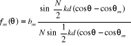 (1.2)
(1.2)
d - inter-element spacing
k - constant
è - angle
l= Nd assumes the array is equal to the
length of the line source. The overall array factor can be written as a
superposition of 2M or 2M+1 terms each of the form of (1.2)
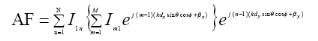
[5]. Therefore Array Factor is defind as
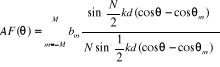 (1.3) (1.3)
Generally, although Woodward-Lawson synthesis technique
reconstructs pattern whose
values at the sampled points are similar to the ones of the
desired signal, it is unable
to control the pattern between the sample points. The quality
of fit to the desired pattern
fd(w) by the synthesis pattern f(w) over the
main beam is measured by the ripple, R,
which is defined as
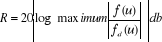 (1.4)
(1.4)
over the main beam. Also of interest is the region between the
main beam and side lobe
region, referred to as the transition region. It is desirable
to have the main beam fall off
shapely into the side lobe region. Thus, the transition width
T is introduced and defined
as  (1.5)
(1.5)
Where wf=0.9 and
wf=0.1 are the values of w where the synthesized
pattern f equals 90%
and 10% of the local discontinuity in the desired pattern
[6].
1.1.2 Dolph-Chebyshev Method
Comparing the Uniform, Dolph-Chebyshev and Binomial
distribution arrays, the uniform amplitude arrays yields the smallest
half-power beamwidth while the binomial arrays usually possess the smallest
side lobes. On the other hand, Dolph- Chebyshev array is mainly a compromise
between uniform and binomial arrays.
Its excitation coefficients are affiliated to the Chebyshev
polynomials and a Dolph-
Chebyshev array with zero side lobes (or side lobes of -8dB)
is simply a binomial design. Thus, the excitation coefficients for this case
would be the same if both methods were used for calculation.
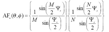
In [6], the array factor of an array of odd and even number of
elements with symmetric excitation is given by
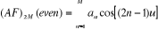 (1.6)
(1.6)
 (1.7) (1.7)
M is an integer, an is the excitation
coefficients and
 (1.8)
(1.8)
The array factor is merely a summation of M or M+1 cosine
terms. The largest harmonic of the cosine terms is one less than the total
number of elements in the array. Each cosine term, whose argument is an integer
times a frequency, can be rewritten as a series of cosine functions with the
fundamental frequency as the argument [5], which is,
m = 0; cos(mu) = 1
m = 1; cos(mu) = cos u
m = 2; cos(mu) = cos (2u) =
2cos2u -1
m = 3; cos(mu) = cos (3u) =
4cos3u - 3cos u
m = 4; cos(mu) = cos (4u) =
8cos4u - 8cos2u + 1 (1.9)
The above are achieved by using the Euler's formula
 (1.10) (1.10)
Where m= number of antennas on x-plane and the trigonometric
identity
sin2u = 1 - cos2u.
Assuming the elements of the array is placed along the z-axis,
and thus, replacing cos u
with z in (1.8), will relate each of the expression to a
Chebyshev polynomial Tm(z).
m = 0; cos(mu) = 1 = T0(z)
m = 1; cos(mu) = z = T1(z)
m = 2; cos(mu) = 2z2
-1 = T2(z)
m = 3; cos(mu) = 4z3 -
3z = T3(z)
m = 4; cos(mu) = 8z4 -
8z2 + 1 = T4(z) (1.11)
These relations between the cosine functions and the Chebyshev
polynomials are valid
only in the range of -1=Z=+1. Because |cos(mu)| =?1,
each Chebyshev polynomial is
|Tm(z)| =1 for -1 =Z =+1. For |z| > 1,
the Chebyshev polynomials are related too the
hyperbolic cosine function [5].
The recursive formula can be used to determine the Chebyshev
polynomial if the polynomials of the previous two orders are known. This is
given by
Tm(z) =
2zTm-1(z) - Tm-2(z)
(1.12)
It can be seen that the array factor of an odd and even number
of elements is a summation of cosine terms whose form is similar with the
Chebyshev polynomials. Therefore, by equating the series representing the
cosine terms of the array to the appropriate Chebyshev polynomial, the unknown
coefficients of the array factor can be determined. Note that the order of the
polynomial should be one less than the total number of elements of the
array.
1.2 Evolution from Omni directional to Smart Antennas
In [7], an antenna in telecommunications system is defined as
a port through which radio frequency (RF) energy is coupled from the
transmitter to the outside world for transmission purposes, and in reverse, to
the receiver from the outside world for reception purposes. To date, antennas
have been the most neglected of all the components in personal communications
systems. Yet, the manner in which radio frequency energy is distributed into
and collected from space has a profound influence upon the efficient use of
spectrum, the cost of establishing new personal communications networks and the
service quality provided by those networks. The goal of the next several
sections is to answer to the question «Why to use anything more than a
single omni directional (no preferable direction) antenna at a base
station?» by describing, in order of increasing benefits, the principal
schemes for antennas deployed at base stations.
1.2.1 Omni directional Antennas
Since the early days of wireless communications, there has
been the simple dipole antenna, which radiates and receives equally well in all
directions (direction here being referred to azimuth). To find its users, this
single-element design broadcasts omni directionally in a pattern resembling
ripples radiation outward in a pool of water (Fig.1.1).
Fig.1.1 Omni directional Antennas and coverage patterns
[7].
While adequate for simple RF environments where no specific
knowledge of the users' whereabouts is either available or needed, this
unfocused approach scatters signals, reaching desired users with only a small
percentage of the overall energy sent out into the environment [8]. Given
this limitation, omni directional strategies attempt to overcome environmental
challenges by simply boosting the power level of the signals broadcast. In a
setting of numerous users (and interferers), this makes a bad situation worse
in that the signals that miss the intended user become interference for those
in the same or adjoining cells. In uplink applications (user to base station),
omni directional antennas offer no preferential gain for the signals of served
users. In other words, users have to shout over competing signal energy [9].
Also, this single-element approach cannot selectively reject signals
interfering with those of served users and has no spatial multipath mitigation
or equalization capabilities. Therefore, omni directional strategies directly
and adversely impact spectral efficiency, limiting frequency reuse. These
limitations of broadcast antenna technology regarding the quality, capacity,
and geographic coverage of mobile communication prompted an evolution in the
fundamental design and role of the antenna in a mobile communication system.
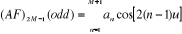
1.2.2 Directional Antennas and Sectorized Systems
A single antenna can also be constructed to have certain fixed
preferential transmission and reception directions. Sectorized antenna systems
take a traditional cellular area and subdivide it into sectors that are covered
using directional antennas looking out from the same base station location Fig.
1.2. Operationally, each sector is treated as a different cell in the system,
the range of which can be greater than in the omni directional case, since
power can be focused to a smaller area. This is commonly referred to as antenna
element gain. Additionally, sectorized antenna systems increase the possible
reuse of a frequency channel in such cellular systems by reducing potential
interference across the original cell. As many as six sectors have been used in
practical service, while more recently up to 16 sectors have been deployed
[10]. However, since each sector uses a different frequency to reduce co
channel interference, handoffs (handovers) between sectors are required.
Narrower sectors give better performance of the system, but this would result
in to many handoffs. While sectorized antenna systems multiply the use of
channels, they do not overcome the major disadvantages of standard omni
directional antennas such as filtering of unwanted interference signals from
adjacent cells.
Fig
1.2: Sectorized antenna system and coverage pattern [10].
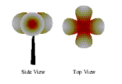
1.2.3 Smart antenna
The smart antenna systems, as shown in Fig 1.3, will be
introduced in order to improve systems performance by increasing spectrum
efficiency, extending coverage area, tailoring beam shaping, steering multiple
beams. Most importantly, smart antenna system increases long-term channel
capacity through Space Division Multiple Access scheme (See
Chapter 4 on Multiple Access Schemes).
In addition, it also reduces multipath fading, co channel
interferences, initial setup cost and bit error rate (BER).
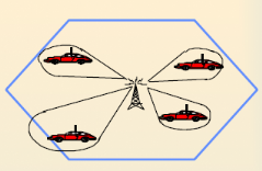
Fig 1.
3: Concept of smart antenna systems [8].
A smart antenna system is defined in [8] as
a system which uses an array of low gain antenna elements with a
signal-processing capability to optimize its radiation and/or reception pattern
automatically in response to the ever changing signal environment.
This can be visualized as the antenna focusing a beam towards
the communication user only.
Truly speaking, antennas are only mechanical construction
transforming free electromagnetic (EM) waves into radio frequency (RF) signals
traveling on a shielded cable or vice-versa. They are not smart but antenna
systems are. The whole system
consists of the radiating antennas, a combining/dividing
network and a control unit. The
control unit is usually realized using a digital signal
processor (DSP), which controls
several input parameters of the antenna to optimize the
communication link.
This show that smart antennas are more than just the
«antenna,» but rather a complete transceiver concept. Smart antenna
systems are customarily classified as either Switching- Beam Array (SBA) or
Adaptive Array (also known as Tracking-Beam Array - TBA) systems and they are
the two different approaches to realizing a smart antenna [1].
1.2.3.1 Switching-Beam Array (SBA)
In the smart antenna systems, the SBA approach forms multiple
fixed beams with
enhanced sensitivity in specific area. These antenna systems
will detect signal strength,
and select one of the best, predetermined, fixed beams for the
subscribers as they move
throughout the coverage sector. Instead of modeling the
directional antenna pattern with
the metallic properties and physical design of a single
element, a SBA system couple
the outputs of multiple antennas in such a manner that it
forms a finely sectorized
(directional) beams with spatial selectivity [10].
Fig 1.4 shows the SBA patterns and Fig 1.5 illustrated the
design network of a typical SBA system. The SBA system network illustrated is
relatively simple to implement, requiring only a beam forming network, a RF
switch, and control logic to select a specific beam.
Fig
1.4 Switch-Beam Systems [11].
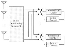
Fig
1.5: A Switch-Beam network [11].
Switched beam systems offer numerous advantages of more
elaborate smart antenna
systems at a fraction of the complexity and expense.
Nevertheless, there are some
limitations to switched beam array, which comprise of the
inability to provide any
protection from multipath components that arrive with
Directions-of-Arrival (DOAs)
near that of the desire components, and also the inability to
take advantage of path
diversity by combining coherent multipath components. Lastly,
due to scalloping, the
received power from a user may fluctuate when he moves around
the base station.
Scalloping is the roll-off of the antenna pattern as a
function of angles as the DOA
varies from the bore sight of each beam produced by the beam
forming network [11].
In spite of the drawbacks, SBA systems are widespread for
various reasons. They
provide some range extension benefits and offer reduction in
delay spread in certain
propagation environments. In addition, the engineering costs
to implement this low
technology approach are lesser than those associated with more
complicated systems.
1.2.3.2 Adaptive Array
From [11], it is reported that it is possible to achieve
greater performance improvements than that obtained using the SBA system. This
can be accomplished by increasing the complexity of the array signal processing
to form the Adaptive Antenna Systems, which is considered to be the most
advance smart antenna approach to date.
The adaptive antenna systems approach communication between a
user and the base station in a different way, in effect adding a dimension in
space. By adapting to the RF
environment as it changes, adaptive antenna technology can
dynamically modify the signal patterns to near infinity to optimize the
performance of the wireless system.
Adaptive arrays continuously differentiate between the desired
signals, multipath, and interfering signals as well as calculate their
directions of arrival by utilizing sophisticated signal-processing algorithms.
The technique constantly updates its transmitting approach based on changes in
both the desired and interfering signal locations. It ensures that signal links
are maximized by tracking and providing users with main lobes and interferers
with nulls, because there are neither micro sectors nor predefined patterns
[12].
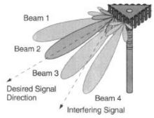
Although both systems seek to increase gain with respect to
the location of the users, however, only the adaptive system is able to
contribute optimal gain while simultaneously identifying, tracking, and
minimizing interfering signals. This can be seen from Fig 1.6 that only the
main lobe is directed towards the user while a null being directed at a co
channel interferer. Illustrated in Fig (1.7) is the network structure of an
adaptive array.
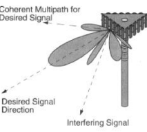
Fig
1.6: An adaptive antenna [11].
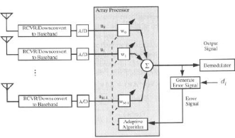
Fig
1.7: Network structure of an adaptive array [11].
CHAP 2 SYSTEM ASPECTS OF SMART
ANTENNA
2.1 Key characteristics of smart antennas Technology
An understanding of signal propagation environment and channel
characteristics is significant to the efficient use of a transmission medium.
In recent years, there have been signal propagation problems associated with
conventional antennas and interference is the major limiting factor in the
performance of mobile communication.
Thus, the introduction of smart antennas is considered to have
the potential of leading to a large increase in mobile communication systems
performance.
A smart antenna system in the mobile communication posses the
following key characteristics:
§ Larger Range Coverage - Smart
antennas provide enhanced coverage through range extension, whole filling, and
better building penetration [13].
§ Reduced Initial Deployment Cost
-When the number of subscribers increases in the network, system capacity
can be increased at the expense of reducing the coverage area and introducing
additional cell sites. Nevertheless, smart antenna can ease this problem by
providing larger early cell sizes and thus, initial deployment cost for the
mobile system can be reduced through range extension [14].
§ ??Reduced Multipath Fading -
The reduction variation of the signal (i.e., fading) greatly enhances system
performance because the reliability and quality of a mobile communications
system can strongly depend on the depth and rate of fading [15].
§ Better Security - The
employment of smart antenna systems diminish the risk of
connection tapping. The intruder must be situated in the
similar direction as the user as seen from the transmitter base station.
§ Better Services - Usage of
the smart antenna system enables the network to have
access to spatial information about the users. This
information can be used to assess the positions of the users much more
precisely than in existing network. This can be applied in services such as
emergency calls and location-specific billing [15].
§ Power efficiency -Combine the inputs
to multiple elements to optimize available processing gain in the downlink
(toward the user)
§ Increased Capacity - Precise
control of signal nulls quality and mitigation of interference combine to
frequency reuse reduce distance improving capacity. Adaptive technologies such
as space division multiple access support the reuse of frequencies within the
same cell [16] [17].
2.2 Signal Propagation: Multipath and cochannel
Interference
2.2.1 Multipath and problem associated
with it.
Multipath is a condition where the transmitted radio signal is
reflected by physical features/structures, creating multiple signal paths
between the base station and the user terminal.
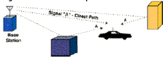
Fig
2.1: The effect of Multipath on a mobile user[8].
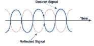
One problem resulting from having unwanted reflected signals
is that the phases of the waves arriving at the receiving station often do not
match. The phase of a radio wave is simply an arc of a radio wave, measured in
degrees, at a specific point in time.
Fig.2.2. illustrates two out-of-phase signals as seen
by the receiver.
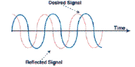
Fig
2.2: Two out-of-Phase Multipath Signal [8].
Conditions caused by multipath that are of primary concern are
as follows:
§ ?Fading: When the waves of multipath
signals are out of phase, reduction in signal strength can occur. One such type
of reduction is called a fade; the phenomenon is known as "Rayleigh fading" or
"fast fading"[8].
A fade is a constantly changing, three-dimensional phenomenon.
Fade zones tend to be small, multiple areas of space within a multipath
environment that cause periodic attenuation of a received signal for users
passing through them. In other words, the received signal strength will
fluctuate downward, causing a momentary, but periodic, degradation in
quality.
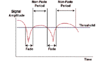
Fig
2.3:.Representation of Fade Effect on User Signal [8].
§ Phase cancellation: When waves of two
multipath signals are rotated to exactly 180° out of phase, the signals
will cancel each other. While this sounds severe, it is rarely sustained on any
given call (and most air interface standards are quite resilient to phase
cancellation). In other words, a call can be maintained for a certain period of
time while there is no signal, although with very poor quality. The effect is
of more concern when the control channel signal is canceled out, resulting in a
black hole, a service area in which call set-ups will occasionally fail [8].
Fig
2.4: Illustration of Phase Cancellation [8].
§ Delay spread: The effect of multipath
on signal quality for a digital air interface (e.g., TDMA) can be slightly
different. Here, the main concern is that multiple reflections of the same
signal may arrive at the receiver at different times. This can result in
intersymbol interference (or bits crashing into one another) that the receiver
cannot sort out.
When this occurs, the bit error rate rises and eventually
causes noticeable degradation in signal quality.
2.2.2 Cochannel
Interference
One of the primary forms of man-made signal degradation
associated with digital radio, co channel interference occurs when the same
carrier frequency reaches the same receiver from two separate transmitters.
Fig
2.5: Illustration of Co channel Interference in a Typical Cellular Grid
[8].
It could be seen that both broadcast antennas as well as more
focused antenna systems scatter signals across relatively wide areas. The
signals that miss an intended user can become interference for users on the
same frequency in the same or adjoining cells [8].
While sectorized antennas multiply the use of channels, they
do not overcome the
major disadvantage of standard antenna broadcast co channel
interference. Management of co channel interference is the number-one limiting
factor in maximizing the capacity of a wireless system. To combat the effects
of co channel interference, smart antenna systems not only focus directionally
on intended users, but in many cases direct nulls or intentional
noninterference toward known, undesired users [13].
2.3 Difference
between uplink and downlink
2.3.1 Uplink Processing
It is assumed here that a smart antenna is only employed at
the base station and not at the handset or subscriber unit. Such remote radio
terminals transmit using omni directional antennas, leaving it to the base
station to separate the desired signals from interference selectively.
Typically, the received signal from the spatially distributed
antenna elements is multiplied by a weight, a complex adjustment of amplitude
and a phase.
These signals are combined to yield the array output. An
adaptive algorithm controls the weights according to predefined objectives. For
a switched beam system, this may be primarily maximum gain; for an adaptive
array system, other factors may receive equal consideration. These dynamic
calculations enable the system to change its radiation pattern for optimized
signal reception [7].
2.3.2 Downlink Processing
The task of transmitting in a spatially selective manner is
the major basis for differentiating between switched beam and adaptive array
systems. As described below, switched beam systems communicate with users by
changing between preset directional patterns, largely on the basis of signal
strength. In comparison, adaptive arrays attempt to understand the RF
environment more comprehensively and transmit more selectively. The type of
downlink processing used depends on whether the communication system uses time
division duplex (TDD), which transmits and receives on the same frequency or
frequency division duplex (FDD), which uses separate frequencies for transmit
and receiving which is the case in GSM system. In most FDD systems, the uplink
and downlink fading and other propagation characteristics may be considered
independent, whereas in TDD systems the uplink and downlink channels can be
considered reciprocal [16]. Hence, in TDD systems uplink channel information
may be used to achieve spatially selective transmission. In FDD systems, the
uplink channel information cannot be used directly and other types of downlink
processing must be considered [7].
2.4 Handling of
common channels
The common channels provide control information for the mobile
stations, considering power levels, access information and so on. This
information has to be transmitted to the whole sector or cell at all time.
Though when designing a base station with smart antennas, it has to be able to
attend to this task. In [20] [21], it is reported that a smart antenna system
consisting of an antenna array, controlled by some weights, might be able to
cover the whole region by employing some special weights for the common
channels. This is a desirable solution, as it only will require some minor
additions to the smart antenna system, and the gain from all the antennas will
be exploited. If a satisfying set of weights can be found, these can be stored
in some non-volatile memory, and recalled each time information is sent on the
common channels.
However if the weights of the antenna array involves that the
whole region can not be covered sufficiently, it might be more feasible to add
an antenna with a wide beam covering the region [22]. The information for the
common channels can then be switched to this antenna. Such a solution is more
expensive, as it requires more hardware, including an antenna, a switch and
possibly an extra transceiver [13].
CHAP 3 ANTENNA ARRAYS AND BEAM FORMING
3.1 Antenna Arrays
3.1.1 Introduction
A directional radiation pattern can be produced when several
antennas are arranged in spaced or interconnected. Such an arrangement of
multiple radiating elements is referred to as an array antenna, or plainly, an
array.
Instead of a single large antenna, many small antennas can be
used in an array to achieve a similar level of performance. The mechanical
problems associated with a single large antenna are traded for the electrical
problems of feeding several small antennas. With the advancements in solid
state technology, the feed network required for array excitation is of improved
quality and reduced cost [10].
Arrays offer the unique ability of electronic scanning of the
main beam, which can be
achieved by altering the phase of the exciting currents in
each element antenna of the
array. Thus, it enables the capability of scanning the
radiation pattern through space.
The array is hereby known as a phased array. Arrays can be of
any form of geometrical
configurations and antenna arrays include the Linear
Array, Planar Array and Circular
Array [23].
The overall field of the array is determined by the vector
addition of the fields radiated by the individual elements and this assumes
that the current in each element is the same as that of the isolated element.
In order to render a very directive pattern, it is essential that the fields
from the elements of the array interfere constructively in the required
directions and interfere destructively in the remaining space.
There are five factors that contribute to the shaping of the
overall pattern of antenna array with identical elements and there are:
§ Geometrical configuration of the array (linear,
circular, rectangular, etc)
§ Displacement between the elements
§ Excitation amplitude of individual elements
§ Excitation phase of individual elements
§ Relative pattern of the individual elements
Some of the above mentioned parameters will thus be used for
our simulations analysis.
In addition, this project will only be covering on linear and
planar arrays.
3.1.2 Theoretical
model for an antenna array
3.1.2.1 Linear array antenna
A linear array of discrete elements is an
antenna consisting of several individuals and indistinguishable elements whose
centers are finitely separated and fall on a straight line
[23]. One dimension uniform linear array is mere and the most
frequently used geometry with the array elements being spaced equally. Fig
(3.1) shows a typical linear array of micro strip antennas, which is one of the
emphases in this final project.
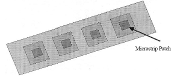
Fig
3.1: Linear array of micro strip [5].
The total field of the array is equal to the field of a single
element positioned at the origin multiple by a factor which is widely known as
the array factor (AF).
The array factor is a function of geometry of the array and
the excitation phase. By varying the separation d and/or the phase
â between the elements, the characteristics of the array factor
and the total field of the array can be controlled [5]. In other words, the
far-zone field of a uniform array with any number of identical elements is:
E(total) = [E(single element at reference point)] X [array
factor] (3.1)
Every array will have its own array factor and thus, the array
factor is generally a function of the number of elements, geometrical sequence,
relative magnitudes, relative phases and the inter-element spacing.
Nevertheless, elements having identical amplitudes, phases and spacing will
result in an array factor of simpler form.
Assuming a N elements array with identical amplitudes
but each succeeding element has a â progressive phase lead
current excitation relative to the preceding one (â represents
the phase by which the current in each element leads the current of the
preceding element). The array factor can thus be obtained by considering the
elements to be point sources. However, if the actual elements are not isotropic
sources, the total field can be form by multiplying the array factor of the
isotropic sources by the field of a single element, which is given by:
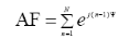 (3.2)
(3.2)
and since the total array factor for the array is a summation
of exponentials, it can be
represented by the vector sum of N phasors each of
unit amplitude and progressive
phase  relative to the previous one [5].
3.1.2.2 Planar array antenna
In addition to placing elements along a straight row to form a
linear array, individual
elements can be positioned along a rectangular grid to form a
rectangular or planar
array, which is capable of providing more variables for
controlling and modeling of
beam pattern. Moreover, planar arrays are also more versatile
with lower side lobe levels
and they can be used to scan the main beam of the antenna
towards any point in space.[6]
Referring to Fig 3.2, the array factor can be derived for a
planar array.
Fig
3.2: Linear and Planar geometries [6].
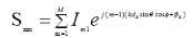
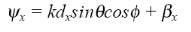
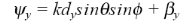
Placing M elements along the x-axis as shown
in Fig 3.2 (i) will have an array factor represented by
 (3.3)
(3.3)
Where: Im1= Excitation coefficient of individual
element
dx= Inter element spacing along x-axis
âx = Progressive phase shift between
elements along x-axis
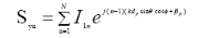
A rectangular array shown in Fig 3.2 (ii) will be formed if
N elements array with a
distance dy apart and with a progressive phase
ây, is placed in the y-direction. Thus, the
array factor for the entire planar array can be written
as[6]
 (3.4)
(3.4)
or,
 (3.5)
(3.5)
where
 (3.6)
(3.6)
 (3.7)
(3.7)
From equation (3.5), it can be seen that the pattern of a
rectangular array is the product of the array factors of the arrays in the
x- and y-plane.
The amplitude of the (m,n)th element can
be written as shown in equation (3.8) if the amplitude excitation coefficients
of the elements of the array in the y-direction are proportional to
those in the x [24],
 (3.8)
(3.8)
However, if the amplitude excitation of the array is uniform
(Imn = Io), then equation
(3.4) can be represented by
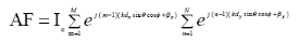 (3.9)
(3.9)
and the normalized form will be
 ( 3.10)
where,
 (3.11)
 (3.12)
The above derivation assumed that each element is an isotropic
source. However, if the
antenna is an array of identical elements, the total field can
be obtained by applying the
pattern multiplication rule of (3.1) in a manner similar as
for the linear array [24].
3.1.3. Elements spacing
The inter-element spacing between the antenna elements is an
important factor in the design of an antenna array. If the elements are more
than ë/2 apart, then the grating lobes appear which degrades the
array performances.
Mutual coupling is an effect that limits the inter-element
spacing of an array. If the elements are spaced closely (typically less than
ë/2), the coupling effects will be larger and generally tend to
decrease with increase in the spacing. Therefore, the elements have to be far
enough to avoid mutual coupling and the spacing has to be smaller than
ë/2 to avoid grating lobes. For all practical purposes, a spacing
of ë/2 is preferred [25].
3.1.4. Microstrip patch antennas design
In the last decade, the patch antenna has become a strong
candidate for the use of the base stations for mobile communication. The patch
is made on a microstrip substrate, and though is an antenna which is easy to
fabricate to handle.
From [22], it is reported that the basic principal of the
patch antenna, is to get electrical fields of the antenna to combine in-phase
in the perpendicular direction of the patch.
For forming an antenna array with a number of patch antennas,
the distance between them is normally given in wavelengths. Some of parameters
constrain for the design, include the length and width of the antenna patch,
the type of substrate used and the substrate thickness. The dimensions of a
rectangular patch antenna can be determined using the following equations as
reported in [22].
 where
W is Width, (3.13) where
W is Width, (3.13)
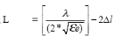 where L is Length (3.14) where L is Length (3.14)
where the effective dielectric constant,
åe and ?l ?are given by:
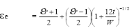 (3.15)
where åe is the effective dielectric and t is
the thickness of the substrate.
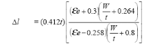 (3.16)
Wavelength, ë?= C/f
Where C is the speed of light, and f is the resonant
frequency.
3.2. Beam forming
A single output of the array is formed when signals induced on
different elements of the array are combined. A plot of the array response as a
function of angle is usually specified as the array pattern or beam pattern. It
can also be known as power pattern when the power response is plotted.
This method of combining the signals from several elements is
understood as beam forming. The direction in which the array has maximum
response is said to be the beam pointing direction, and thus this is the
bearing where the array has the utmost gain.
Conventional beam pointing or beam forming can be achieved by
adjusting only the phase of the signals from different elements. In other
words, pointing a beam in the desired direction. However, the shape of the
antenna pattern in this case is fixed, that is, the side lobes with respect to
the main do not change when the main beam is pointed in different directions by
adjusting various phases. Nevertheless, this can be overcome by adjusting the
gain and phase of each signal to shape the pattern as required and the degree
of change will depend upon the number of elements in the array [26].
For example, signals can also be coupled together without any
gain or phase shift in a linear array, and it is known as broadside to the
array, which is, perpendicular to the row joining all the elements of the
array. The array pattern formed thus falls to a low value on either side of the
beam pointing direction and the region of the low value is known as a null. In
this case, it must be noted that the null is actually a position where the
array response is zero and the term should not be misused to denote the low
value of the pattern.
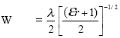
Lastly, it is very convenient to make use of vector notation
while working with array antennas. Thus the term weight vector (W) is
introduced. It is important because the weight vector will have significant
impact on the array output.
3.2.1. Nulling Beam Forming
The flexibility of array weighting to being adjusted to
specify the array pattern is an important property. This may be exploited to
cancel directional sources operating at the same frequency as that of the
desired source, provided these are not in the direction of the desired source
[26].
In circumstances where the directions of these interferences
are identified, cancellation is feasible by positioning the nulls in the
pattern corresponding to these directions and concurrently steering the main
beam in the direction of the desired signal. This approach of beam forming by
placing nulls in the directions of interferences is commonly referred to as
null beam forming or null steering [27].
3.2.2. Steering Vector
The steering vector contains the response of all elements of
the array to a narrow-band source of unit power. As the response of the array
is different in different directions, a steering vector is associated with each
directional source. The uniqueness of this
Association depends upon the array geometry [26]. Every
component of this vector has unit magnitude for an array of identical elements.
The phase of its i th component is similar to the
phase difference between signals induced on the ith
element and the reference element due to the source associated with the
steering vector. This vector is also known as the space vector because each
component of the vector represents the phase delay that is resulted from the
spatial position of the corresponding element of the array. In addition, it can
also be referred to as the array response vector for it measures the response
of the array due to the source under consideration.
Beam forming is used by the smart antennas, in order to obtain
a radiation pattern which only receives from and transmits to the desired
directions, while attenuating undesired directions. The only available
information for downlink transmission is the directional to the mobile station.
It is furthermore reasoned that in that situation, it is desired to send as
much power in the direction of the mobile station as possible, attenuating all
other directions. Most of basic beam forming methods, point the antenna beam in
a certain direction, by applying phase shifts to the signals to the individuals
antenna in the array. [28]. The phase shifts can be applied in same digital
baseband.
3.2.3. Recursive Least Squares Algorithm
Because the environment (e.g. mobileenvironment) is
time-variable, it is essential that the weight vector to be updated or adapted
periodically for an adaptive array network. As the necessary data to estimate
the optimal solution is noisy, an adaptive algorithm is exploited for updating
the weight vector periodically. In [22], it is reported that there are many
types of adaptive algorithms and the majorities are iterative. They utilized
the past information to minimize the computations required at each updatecycle.
In iterative algorithms, the current weight vector, W(n), is modified
by an incremental value to form a new weight vector,W(n+1) at each
iteration n. The RLS algorithm is summarized as follow [22]:
Initialization
 (3.17)
W(0) = 0 (3.18)
Weight Update
 (3.19)
 (3.20)
 (3.21)
 (3.22)
Convergence coefficient
0<ë<1, where;
ä is a small positive number,
I is the MXM identity matrix,
ë is the forgetting factor
k(n) is the gain vector,
á(n) is the innovation,
W(n) is the weight vector,
P(n) is the inverse of the correlation matrix Ô(n),
u(n) is the input vector
d(n) is the desired response.
In the RLS method, the desired signal must be supplied using
either a training sequence
or decision direction. For the training sequence approach, a
brief data sequence is transmitted which is known by the receiver. The receiver
uses the adaptive algorithm to
approximate the weight vector in the training duration, then
retains the weights constant
while information is being transmitted. This technique
requires that the environment be
stationary from one training period to the next, and it
reduces channel throughput by requiring the use of channel symbols for
training. However, in the decision approach, the receiver uses recreated
modulated symbols based on symbol decisions, which are used as the desired
signal to adapt the weight vector [22].
CHAP 4 Multiple
Access Schemes
4.1 Introduction
The Multiple Access Scheme defines how the radio frequency can
be shared by different simultaneous communication between different mobile
stations located in different cells [29]. The distribution of spectrum is
required to achieve this high system capacity by simultaneously allocating the
available bandwidth (or available amount of channels) to multiple users. In
this chapter, we discuss four access schemes used to share the available
bandwidth in a wireless communication. Nonetheless, they are known as the
frequency division multiple access (FDMA), time division multiple access
(TDMA), code division multiple access (CDMA) and Space division multiple access
(SDMA). As a result, there is a lot to debate about which schemes is better to
use in smart antennas systems. However, as it is reported in [30], the answer
to this depends on the combined techniques, such as the modulation scheme,
anti-fading techniques, forward error correction, and so on, as well as the
requirements of services, such as the coverage area, capacity, traffic, and
types of information.
4.2 Frequency Division Multiple Access (FDMA)
In FDMA, the bandwidth of the available spectrum is divided
into separate channels, each individual channel frequency being allocated to a
different user for transmission [28]. When a user sends a call request, the
system will assign one of the available channels to the user, in which, the
channel is used exclusively by that user during a call. However, the system
will reassign this channel to a different user when the previous call is
terminated.
Fig
4.1: Concept of FDMI system
4.3 Time Division Multiple Access (TDMA)
In TDMA the same spectrum channel frequency is shared
by all users, but each is only permitted to transmit in short bursts of time
(slots), thus sharing the channel between all the remote stations by dividing
it over time [28].
Fig
4.2: Concept of TDMA system
4.4 Code Division Multiple Access (CDMA)
In a CDMA system all users occupy the same frequency,
and there are separated from each by means of a special code. Each user is
assigned a code applied as a secondary modulation, which is used to transform
user's signal into spread-spectrum-coded version of the user's data stream. The
receiver then uses the same spreading code to transform the spread-spectrum
signal back into the original user's data stream [28].
Fig
4.3: Concept of a CDMA system
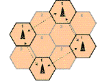
4.4 Space Division Multiple Access (SDMA)
In spatial division multiple access (SDMA), multiple mobiles
can communicate with a single base station on the same frequency. By using
highly directional beams and/or forming nulls in the directions of all but one
of the mobiles on a frequency, the base station creates multiple channels using
the same frequency, but separated in space [31].
![]()
Fig 4.4 Concept of SDMA system
CHAP 5 SIMULATION USING MATLAB
5.1 Analysis and Simulation on array antenna
This section will be exploring the radiation patterns of a
planar array by varying various parameters. The parameters include the
inter-element spacing, number of elements in the array and the amplitude
distribution. The subsequent simulations on planar array are performed using
the MATLAB 6.5.1. The element polarization is assumed to be in the x-
plane.
Appendix provides the MATLAB code we used.
5.1.1 Variation of number of elements
N
The following assumptions are made for the investigation:
§ Normalized inter-element spacing = 0.5
§ Side lobe level = 20dB
. Fig 5.1, Fig 5.2 and Fig.5.3 illustrate the plot generated
from MATLAB
Fig 5.1
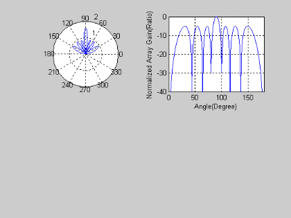
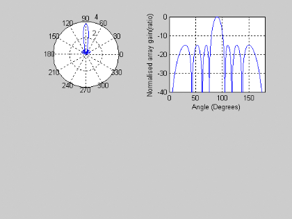
: Radiation pattern with 4 elements
Fig 5.2
Radiation pattern with 8 elements
Fig 5.3
: Radiation pattern with 10 elements
Observed results are tabulated in Table 1
|
Number of elements
|
Remarks
|
|
2
|
Main Beam with no side lobe
|
|
4
|
2sidelobes appear
|
|
6
|
4sidelobes appear
|
|
8
|
6sidelobes appear
|
|
10
|
8sidelobes appear
|
Table 1 :Results of varying number
of elements
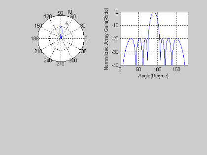
5.1.2 Variation of Side Lobe Level
The following assumptions are made for the synthesis:
§ Normalized inter-element spacing = 0.5
§ Number of elements = 8
Plot generated from MATLAB are following
Fig
5.4: Radiation pattern with 5dB.
Fig
5.5: Radiation pattern with 15dB
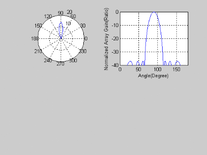
Fig
5.6: Radiation pattern with 37dB
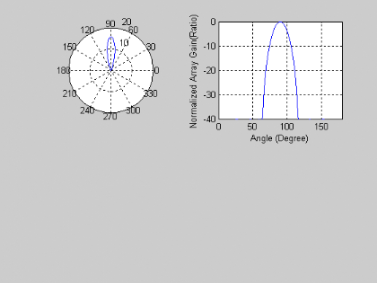
Fig
5.7: Radiation pattern with 40dB
Observed results are tabulated in Table 2.
|
Side lobe level(dB)
|
Remarks
|
|
5
|
6 side lobes appear
|
|
10
|
6 side lobes appear
|
|
15
|
6 side lobes appear
|
|
20
|
6 side lobes appear
|
|
25
|
6 side lobes appear
|
|
30
|
6 side lobes appear
|
|
40
|
6 side lobes appear
|
Table 2: Results of varying side
lobe level
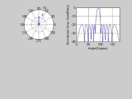
5.1.3 Variation of Inter-element
Spacing.
This section will be analyzing on the radiation pattern for
various inter-element spacing.
First and foremost, the following assumption is made:
§ Side lobe level = 20dB
§ Number of elements =8
The data obtained was tabulated in Table 3
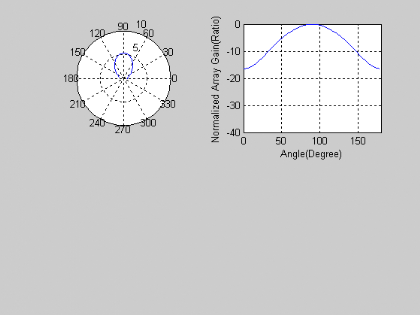
Fig 5.8
Radiation Pattern with normalized inter-element spacing of 0.125
Fig
5.9: Radiation Pattern with normalized inter-element spacing of 0.5
Fig
5.10: Radiation Pattern with normalized inter- element spacing of 0.75
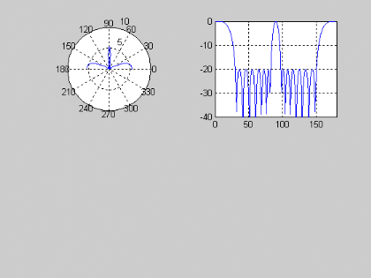
Fig 5.11 Radiation Pattern with
normalized inter-element spacing of 1
Observed results are tabulated below.
|
Number of elements
|
Inter-element spacing(Normalized)
|
Remarks
|
|
8
|
0.125
|
Main Beam with no side lobe
|
|
8
|
0.25
|
2 side lobes appear
|
|
8
|
0.375
|
6 side lobes appear
|
|
8
|
0.5
|
6sidelobes appear
|
|
8
|
0.625
|
8sidelobes appear
|
|
8
|
0.75
|
10sidelobes appear
|
|
8
|
0.825
|
14sidelobes appear
|
|
8
|
1
|
2grating lobes and12 side lobes appear
|
Table 3 : Results of varying
inter-element spacing
5.2 Discussion
From analysis results, a narrow 3dB beamwidth is achieved by
increasing the number of elements in the arrays for a fixed side lobe level.
Simulations show that the number of side lobes increases with
that of elements, but the side lobe level remains constant.
The beamwidth increases when the side lobe level decreases for
a fixed number of elements and inter-elements spacing, but the number of side
lobes doesn't change.
As the inter-elements spacing increases, the beamwidth
decreases. Thus, he number of side lobes multiples.
There is a generation of grating lobes when the inter-elements
spacing is equal to the wavelength.
Last but not least, the result shows that this synthesis can
be applied for achieving a narrow beamwidth accompanied by low side lobes
level.
CONCLUSION AND
RECOMMANDATIONS.
By giving an introduction to basic antenna theory, this
project had led to a better understanding of antennas with emphasis on array
antennas.
The evolution path from omni directional to the smart antenna
system was shown before proving the switching-beam array and adaptive array
approaches i.e. classifications of smart antenna.
A detailed description on system aspect of smart antenna was
presented and it includes the benefits of smart antenna system, multipath and
problems associated with it.
Various schemes such as FDMA, TDMA, CDMA and SDMA could be
utilized to exploit the range of frequencies available for mobile communication
technologies.
Radiation pattern and performance of array antennas have been
investigated. Simulation results show that the radiation pattern depends on the
number of elements in the array, the inter-elements spacing, and an amplitude
distribution. Thus, there is always a compromise between the influencing
parameters.
In conclusion, the project shows that smart antennas offer
several possibilities than omni directional or sector antennas. They increase
coverage through range extension, capacity through interference reduction or
SDMA, and mitigation of multipath fading and intersymbol interference. They can
be integrated in a given base station without any change on the adjacent cell
or on the mobile station.
Because of the key characteristics presented above, smart
antennas system are recommended to mobile communications companies to be used
especially in big towns where the number of subscribers is large.
However, further studies are required for the future of mobile
dimension. This project covers only two methods; Dolph-Chebychev and
Woodward-Lawson method, but Fourier Transform and Taylor Line-Source methods
may be used also in other research.
References
[1]. G.T. Okamato: Smart Antenna Systems and Wireless
LANs. Kluwer
Academic, Massachusettes, 1999.
[2]. Dr.Felix Akorli, Antenna and Waves Propagations. Class
notes, NUR, 2004
[3]. W.C. Jakes, Jr., et al, Microwave Mobile
Communications. New York:
Wiley, 1974.
[4]. K.F. Lee: Principles of Antenna Theory. John
Wiley & Sons, New York,
1984.
[5]. C.A. Balanis: Antenna Theory. John Wiley &
Sons, New York, 1997
[6]. W.S. Strutzman and G.A. Thiele: Antenna Theory and
Design, John Wiley
& Sons, New York, 1981.
[7]. M. Cooper and M. Goldburg ,Intelligent Antennas
Apatial Division
Multiple Acces. New York, 1996.
[8]. Smart Antenna System, Web proforum Tutorial, The
Imternational
Engineering Consortium,
http://www.iec.org, May 07, 2005
[9].J. H. Winters, «Optimum combining for indoor radio
systems with multiple
users,» IEEE Trans. Commun., vol..
COM-35, no. 11, Nov. 1987
[10]. IoWave Inc. Smart Antenna.
http://www.iowave.com/, June 23, 2005
[11].
http://www.ececs.uc.edu/~radhakri/Research.htm/,
August 16,2005
[12]. J. H. Winters, «Signal Acquisition and Tracking
with Adaptive Arrays in
the Digital Mobile Radio System IS-54 with flat
fading», IEEE Trans. Veh.
Technol., vol. 42, no. 4, Nov. 1993
[13]. Ole Norklit and Jorgen B.Andersen, Mobile radio
environments and
adaptive arrays. Denmark,1994.
[14]. T.S. Rappaport: Wireless Communications: Principles
& Practice.
Prentice Hall, Upper Saddle River, New Jersey,
1996.
[15]. P.H. Lehne and M. Pettersen, An Overview of Smart
Antenna Technology
for Mobile Communications System. Surveys,
http://www.comsoc.org/pubs/surveys/4q99issue/lehne.html,
September 13,
2005
[16]. R. Prasad: CDMA for Wireless Personal
Communications, Artech House,
Boston, 1996.
[17]. Per H. Lehne and Mangne Pettersen. «An Overview of
Smart Antenna
Technology for Mobile Communication Systems».
IEEE Communications
Surveys, 2(4):2-13, Fourth Quarter 1999
[18]. P.G. Proakis, Digital Comunications. New York:
McGraw-Hill, 1983
[19]. Nowicki and J. Roumeliotos. Smart Antenna Strategies
for Mobile
Communications, April 1995
[20]. Ng K. Chong, O. K. Leong, P. R. P. Hoole, and E. Gunawan
Smart Antennas and Signal. 2001.
[21]. Rodney G. Vaughan Antenna diversity in landmobile
communication. 1985.
[22]. J.C. Liberti Jr. and T.S. Rappaport: Smart Antennas
for Wireless
Communications: IS-95 and Third Generation CDMA
Applications.
Prentice Hall, Upper Saddle River, New Jersey,
1999.
[23]. M.T. Ma: Theory and Application of Antenna
Arrays. John wiley & Sons,
New York, 1974.
[24]. T. Macnamara: Handbook of Antennas for EMC.
Artech House, London,
1995
[25]. Ole Norklit and Jorgen B.Andersen,Mobile radio
environments and
adaptive arrays. Denmark,1994
[26]. L.C. Godara, «Applications of Antenna Arrays to
Mobile Communication,
Part I: Performance, Improvement, Feasibility and
Systems
Considerations» Proceedings of the
IEEE, Vol. 85, No. 7, Jul. 1997, pp.
1029-1060
[27]. J. John Litva, Titus Lo, Digital Beam forming in
Wireless
Communications. Norwood:Artech House,
1996
[28].
www.eecg.tronto.edu, September 13,
2005
[29]. Dr.Felix Akorli, Radar and Satellite Communications.
Class notes,NUR,
2004
[30]. S. Sampei: Applications of Digital Wireless
Technologies to Global Wireless
Communications. Prentice Hall, Upper Saddle
River, New Jersey, 1997.
[31].
http://schola.lib.vt.edu/theses/available/etd-04262000-
15330030/unrestricted/ch10.pdf, August 05, 2005
APPENDIX
clc; % Clear screen
clear; % Clear all variables
load C:\MATLAB6p5p1\work\DATAS.dat % Read data in the input
file
g=5;
for i=1:g,
N = DATAS(i,1);% Prompt for number of elements in an array.
SLL = DATAS(3,2);% Prompt for the required Side Lobe
Level.
R = 10.^(SLL/20); % Convert to ratio
Zo = cosh((1/(N-1))*acosh(R)); % Determine Zo
spacing = DATAS(3,3);% Prompt for the Normalised
Inter-element Spacing.
t = 0:1:179;
theta = t*pi/180; % Convert to radian
u = pi*spacing*cos(theta);
if N == 2;
AFp = [1]; % Polynomial of excitation coefficient
AFc = [1*Zo]; % Chebyshev polynomial
X = AFp\AFc; % Determine the excitation coefficient
Xo = X/X(1,1); % Normalized with respect to the amplitude of
the elements at the edge
AF = abs(Xo(1,1)*cos(u)); % Determine the array factor
subplot(2,2,1);
polar(theta,AF); % Generate polar plot
AF1=20*log10(AF); % Convert to decibels
max=max(AF1); % Setting maximum value of the array factor to
"max"
AF2=AF1-max; % Set values of array factor with respect to
maximum value
theta1=(180/pi)*theta;
subplot(2,2,2);
plot(theta1,AF2); % Generate linear plot
axis([0 180 -40 0]); % Set maximum and minimum values for X
and Y scales
title('RADIATION PATTERN WITH 2 ELEMENTS');
xlabel('Thetal');
ylabel('Array Factor')
grid; % Turn grid on
pause
clear; % Clear all variables
load C:\MATLAB6p5p1\work\DATAS.dat % Read data in the input
file
elseif N == 3;
AFp = [0,2;
1,-1]; % Polynomial of excitation coefficient
AFc = [2*Zo^2; % Chebyshev polynomial
-1];
X = AFp\AFc; % Determine the excitation coefficient
Xo = X/X(2,1); % Normalized with respect to the amplitude of
the elements at the edge
AF = abs(Xo(1,1)+Xo(2,1)*cos(2*u));% Determine the array
factor
subplot(2,2,1);
polar(theta,AF); % Generate polar plot
AF1=20*log10(AF); % Convert to decibels
max=max(AF1); % Setting maximum value of the array factor to
"max"
AF2=AF1-max; % Set values of array factor with respect to
maximum value
theta1=(180/pi)*theta;
subplot(2,2,2);
plot(theta1,AF2); % Generate linear plot
axis([0 180 -40 0]); % Set maximum and minimum values for X
and Y scales
grid % Turn grid on
pause
clear; % Clear all variables
load C:\MATLAB6p5p1\work\DATAS.dat % Read data in the input
file
elseif N==4;
AFp = [0,4;
1,-3]; % Polynomial of excitation coefficient
AFc = [4*Zo^3;
-3*Zo]; % Chebyshev polynomial
X = AFp\AFc; % Determine the excitation coefficient
Xo = X/X(2,1); % Normalized with respect to the amplitude of
the elements at the edge
AF = abs(Xo(1,1)*cos(u)+Xo(2,1)*cos(3*u));% Determine the
array factor
subplot(2,2,1);
polar(theta,AF); % Generate polar plot
AF1=20*log10(AF); % Convert to decibels
max=max(AF1); % Setting maximum value of the array factor to
"max"
AF2=AF1-max; % Set values of array factor with respect to
maximum value
theta1=(180/pi)*theta;
subplot(2,2,2);
plot(theta1,AF2); % Generate linear plot
axis([0 180 -40 0]); % Set maximum and minimum values for X
and Y scales
title('RADIATION PATTERN WITH 4 ELEMENTS');
xlabel('Thetal');
ylabel('Array Factor')
grid % Turn grid on
pause
clear; % Clear all variables
load C:\MATLAB6p5p1\work\DATAS.dat % Read data in the input
file
elseif N == 5;
AFp = [0,0,8;
0,2,-8;
1,-1,1]; % Polynomial of excitation coefficient
AFc = [8*Zo^4;
-8*Zo^2;
1]; % Chebyshev polynomial
X = AFp\AFc; % Determine the excitation coefficient
Xo = X/X(3,1); % Normalized with respect to the amplitude of
the elements at the edge
AF = abs(Xo(1,1)+Xo(2,1)*cos(2*u)+Xo(3,1)*cos(4*u));%
Determine the array factor
subplot(2,2,1);
polar(theta,AF); % Generate polar plot
AF1=20*log10(AF); % Convert to decibels
max=max(AF1); % Setting maximum value of the array factor to
"max"
AF2=AF1-max; % Set values of array factor with respect to
maximum value
theta1=(180/pi)*theta;
subplot(2,2,2);
plot(theta1,AF2); % Generate linear plot
axis([0 180 -40 0]); % Set maximum and minimum values for X
and Y scales
grid % Turn grid on
pause
clear; % Clear all variables
load C:\MATLAB6p5p1\work\DATAS.dat % Read data in the input
file
elseif N==6;
AFp = [0,0,16;
0,4,-20;
1,-3,5,]; % Polynomial of excitation coefficient
AFc = [16*Zo^5;
-20*Zo^3;
5*Zo]; % Chebyshev polynomial
X = AFp\AFc; % Determine the excitation coefficient
Xo = X/X(3,1); % Normalized with respect to the amplitude of
the elements at the edge
AF = abs(Xo(1,1)*cos(u)+Xo(2,1)*cos(3*u)+Xo(3,1)*cos(5*u));%
Determine the array factor
subplot(2,2,1);
polar(theta,AF); % Generate polar plot
AF1=20*log10(AF); % Convert to decibels
max=max(AF1); % Setting maximum value of the array factor to
"max"
AF2=AF1-max; % Set values of array factor with respect to
maximum value
theta1=(180/pi)*theta;
subplot(2,2,2);
plot(theta1,AF2); % Generate linear plot
axis([0 180 -40 0]); % Set maximum and minimum values for X
and Y scales
title('RADIATION PATTERN WITH 6 ELEMENTS');
xlabel('Thetal');
ylabel('Array Factor')
grid % Turn grid on
pause
clear; % Clear all variables
load C:\MATLAB6p5p1\work\DATAS.dat % Read data in the input
file
elseif N == 7;
AFp = [0,0,0,32;
0,0,8,-48;
0,2,-8,18
1,-1,1,-1]; % Polynomial of excitation coefficient
AFc = [32*Zo^6;
-48*Zo^4;
18*Zo^2;
-1]; % Chebyshev polynomial
X = AFp\AFc; % Determine the excitation coefficient
Xo = X/X(4,1); % Normalized with respect to the amplitude of
the elements at the edge
AF
=abs(Xo(1,1)+Xo(2,1)*cos(2*u)+Xo(3,1)*cos(4*u)+Xo(4,1)*cos(6*u));% Determine
the array factor
subplot(2,2,1);
polar(theta,AF); % Generate polar plot
AF1=20*log10(AF); % Convert to decibels
max=max(AF1); %Setting maximum value of the array factor to
"max"
AF2=AF1-max; % Set values of array factor with respect to
maximum value
theta1=(180/pi)*theta;
subplot(2,2,2);
plot(theta1,AF2); % Generate linear plot
axis([0 180 -40 0]); % Set maximum and minimum values for X
and Y scales
grid % Turn grid on
pause
clear; % Clear all variables
load C:\MATLAB6p5p1\work\DATAS.dat % Read data in the input
file
elseif N==8;
AFp = [0,0,0,64;
0,0,16,-112;
0,4,-20,56;
1,-3,5,-7,]; % Polynomial of excitation coefficient
AFc = [64*Zo^7;
-112*Zo^5;
56*Zo^3;
-7*Zo]; % Chebyshev polynomial
X = AFp\AFc; % Determine the excitation coefficient
Xo = X/X(4,1); % Normalized with respect to the amplitude of
the elements at the edge
AF
=abs(Xo(1,1)*cos(u)+Xo(2,1)*cos(3*u)+Xo(3,1)*cos(5*u)+Xo(4,1)*cos(7*u));%
Determine the array factor
subplot(2,2,1);
polar(theta,AF); % Generate polar plot
AF1=20*log10(AF); % Convert to decibels
max=max(AF1); % Setting maximum value of the array factor to
"max"
AF2=AF1-max; % Set values of array factor with respect to
maximum value
theta1=(180/pi)*theta;
subplot(2,2,2);
plot(theta1,AF2); % Generate linear plot
axis([0 180 -40 0]); % Set maximum and minimum values for X
and Y scales
grid % Turn grid on
title('RADIATION PATTERN USING 8 ELEMENTS');
xlabel('Thetal');
ylabel('Array Factor')
mytable=fopen('RESULTS.txt','wt'); %open ouput file for
writing
fprintf(mytable, 'THETAL\tARRAY FACTOR\n');
A=[theta1];
B=[AF2];
for p=0:1:179
for q=p,
fprintf(mytable, '%.2f\t %.2f\n', A(p), B(q));
fclose (mytable);
end
end
pause
clear; % Clear all variables
load C:\MATLAB6p5p1\work\DATAS.dat
elseif N == 9;
AFp = [0,0,0,0,128;
0,0,0,32,-256;
0,0,8,-48,160;
0,2,-8,18,-32;
1,-1,1,-1,1]; % Polynomial of excitation coefficient
AFc = [128*Zo^8;
-256*Zo^6;
160*Zo^4;
-32*Zo^2;
1]; % Chebyshev polynomial
X = AFp\AFc; % Determine the excitation coefficient
Xo = X/X(5,1); % Normalized with respect to the amplitude of
the elements at the edge
AF
=abs(Xo(1,1)+Xo(2,1)*cos(2*u)+Xo(3,1)*cos(4*u)+Xo(4,1)*cos(6*u)+Xo(5,1)*cos(8*u));
subplot(2,2,1);
polar(theta,AF); % Generate polar plot
AF1=20*log10(AF); % Convert to decibels
max=max(AF1); % Setting maximum value of the array factor to
"max"
AF2=AF1-max; % Set values of array factor with respect to
maximum value
theta1=(180/pi)*theta;
subplot(2,2,2);
plot(theta1,AF2); % Generate linear plot
axis([0 180 -40 0]); % Set maximum and minimum values for X
and Y scales
grid % Turn grid on
pause
clear; % Clear all variables
load C:\MATLAB6p5p1\work\DATAS.dat
elseif N==10;
AFp = [0,0,0,0,256;
0,0,0,64,-576;
0,0,16,-112,432;
0,4,-20,56,-120;
1,-3,5,-7,9]; % Polynomial of excitation coefficient
AFc = [256*Zo^9;
-576*Zo^7;
432*Zo^5;
-120*Zo^3;
9*Zo]; % Chebyshev polynomial
X = AFp\AFc; % Determine the excitation coefficient
Xo = X/X(5,1); % Normalized with respect to the amplitude of
the elements at the edge
AF
=abs(Xo(1,1)*cos(u)+Xo(2,1)*cos(3*u)+Xo(3,1)*cos(5*u)+Xo(4,1)*cos(7*u)+Xo(5,1)*cos(9*u));
subplot(2,2,1);
polar(theta,AF); % Generate polar plot
AF1=20*log10(AF); % Convert to decibels
max=max(AF1); % Setting maximum value of thearray factor to
"max"
AF2=AF1-max; % Set values of array factor with respect to
maximum value
theta1=(180/pi)*theta;
subplot(2,2,2);
plot(theta1,AF2); % Generate linear plot
axis([0 180 -40 0]); % Set maximum and minimum values for X
and Y scales
grid % Turn grid on
title('RADIATION PATTERN WITH 10 ELEMENTS');
xlabel('Thetal');
ylabel('Array Factor')
end
end
pause
clc; % Clear screen
clear; % Clear all variables
% Prompt for number of elements in an array.
load C:\MATLAB6p5p1\work\DATAS.dat
% Prompt for the required Side Lobe Level.
h=5;
for j=1:h,
SLL = DATAS(j,2);
R = 10.^(SLL/20); % Convert to ratio
N = DATAS(4,1);
Zo = cosh((1/(N-1))*acosh(R)); % Determine Zo
spacing = DATAS(3,3);% Prompt for the Normalised
Inter-element Spacing.
t = 0:1:179;
theta = t*pi/180; % Convert to radian
u = pi*spacing*cos(theta);
if N==8;
AFp = [0,0,0,64;
0,0,16,-112;
0,4,-20,56;
1,-3,5,-7,]; % Polynomial of excitation coefficient
AFc = [64*Zo^7;
-112*Zo^5;
56*Zo^3;
-7*Zo]; % Chebyshev polynomial
X = AFp\AFc; % Determine the excitation coefficient
Xo = X/X(4,1); % Normalized with respect to the amplitude of
the elements at the edge
AF
=abs(Xo(1,1)*cos(u)+Xo(2,1)*cos(3*u)+Xo(3,1)*cos(5*u)+Xo(4,1)*cos(7*u));%
Determine the array factor
subplot(2,2,1);
polar(theta,AF); % Generate polar plot
AF1=20*log10(AF); % Convert to decibels
max=max(AF1); % Setting maximum value of the array factor to
"max"
AF2=AF1-max; % Set values of array factor with respect to
maximum value
theta1=(180/pi)*theta;
subplot(2,2,2);
plot(theta1,AF2); % Generate linear plot
axis([0 180 -40 0]); % Set maximum and minimum values for X
and Y scales
grid % Turn grid on
title('RADIATION PATTERN WITH VARIATION OF SLL');
xlabel('Thetal');
ylabel('Array Factor')
pause
clear; % Clear all variables
% Prompt for number of elements in an array.
load C:\MATLAB6p5p1\work\DATAS.dat
end
end
clc; % Clear screen
clear; % Clear all variables
load C:\MATLAB6p5p1\work\DATAS.dat
SLL = DATAS(3,2);% Prompt for the required Side Lobe
Level.
R = 10.^(SLL/20); % Convert to ratio
N = DATAS(4,1);
Zo = cosh((1/(N-1))*acosh(R)); % Determine Zo
m=5;
for u=1:m,
load C:\MATLAB6p5p1\work\DATAS.dat
spacing = DATAS(u,3);% Prompt for the Normalised
Inter-element Spacing.
t = 0:1:179;
theta = t*pi/180; % Convert to radian
u = pi*spacing*cos(theta);
N = DATAS(4,1);
if N==8;
AFp = [0,0,0,64;
0,0,16,-112;
0,4,-20,56;
1,-3,5,-7,]; % Polynomial of excitation coefficient
SLL = DATAS(3,2);
R = 10.^(SLL/20); % Convert to ratio
Zo = cosh((1/(N-1))*acosh(R)); % Determine Zo
AFc = [64*Zo^7;
-112*Zo^5;
56*Zo^3;
-7*Zo]; % Chebyshev polynomial
X = AFp\AFc; % Determine the excitation coefficient
Xo = X/X(4,1); % Normalized with respect to the amplitude of
the elements at the edge
AF
=abs(Xo(1,1)*cos(u)+Xo(2,1)*cos(3*u)+Xo(3,1)*cos(5*u)+Xo(4,1)*cos(7*u));
subplot(2,2,1);
polar(theta,AF); % Generate polar plot
AF1=20*log10(AF); % Convert to decibels
max=max(AF1); % Setting maximum value of the array factor to
"max"
AF2=AF1-max; % Set values of array factor with respect to
maximum value
theta1=(180/pi)*theta;
subplot(2,2,2);
plot(theta1,AF2); % Generate linear plot
axis([0 180 -40 0]); % Set maximum and minimum values for X
and Y scales
grid % Turn grid on
title('RADIATION PATTERN WITH VARIATION OF INTER ELEMENTS
SPACING');
xlabel('Thetal');
ylabel('Array Factor')
pause
clear; % Clear all variables
end
end
 
| 

