|
THE EFFECT OF LAND FRAGMENTATION ON THE PRODUCTIVITY
AND TECHNICAL EFFICIENCY OF SMALLHOLDER MAIZE FARMS IN SOUTHERN
RWANDA
BY
KARANGWA MATHIAS, B.A Economics (National University of
Rwanda)
A THESIS SUBMITTED TO THE GRADUATE SCHOOL FOR THE AWARD
OF A DEGREE OF MASTER OF SCIENCE IN AGRICULTURAL AND APPLIED ECONOMICS OF
MAKERERE UNIVERSITY
SEPTEMBER 2010
DECLARATION
I, Mathias Karangwa, hereby declare that this thesis is my
original work and has never been submitted to any other academic institution
for the award of a degree.
Mathias Karangwa
..............................................................
This thesis has been submitted to the school of graduate
studies of MAKERERE UNIVERSITY with the approval of the following
supervisors:
Dr. Fredrick Bagamba PhD (Agricultural
Economics)............................
Date.............................................................
Dr. Bernard Bashaasha PhD (Agricultural
Economics)...........................
Date...........................................................
(c) MAKERERE UNIVERSITY
DEDICATION
This thesis is dedicated to my late mother, Rose Buhinja
ACKNOWLEDGEMENT
I primarily acknowledge my Supervisors, Dr. Fredrick Bagamba
and Dr. Bernard Bashaasha for their friendly and useful advice, guidance and
corrections that helped me to complete this work.
My sincere thanks are extended to the Germany Academic
Exchange Service/Deutscher Akademischer Austausch Dienst (DAAD), the African
Economics Research Consortium (AERC) and the Collaborative Master's program in
Agricultural and Applied Economics (CMAAE) for the financial support.
Finally, I thank all the staff of the Department of
Agricultural Economics and Agribusiness, Faculty of Agriculture, Makerere
University for the knowledge they imparted in me throughout the two years I
stayed at this institution. I am grateful to my classmates, with whom I shared
knowledge and experiences.
TABLE OF CONTENTS
LIST OF TABLES
LIST OF FIGURES
ABSTRACT
The government of Rwanda believes that land fragmentation is a
major threat to efficient crop production in the country due to the fact that
continuous subdivision of farms has led to small sized land holdings that may
be hard to economically operate. This study analyzed the determinants of the
productivity and technical efficiency of smallholder maize farms in Gisagara
district with a particular focus on land fragmentation using plot size, number
of plots per household and distance from the households' residences to plots as
measures of land fragmentation. Gisagara district was chosen because previous
empirical studies showed high land fragmentation there. The main objective of
this study was to determine the effect of the various dimensions of land
fragmentation on the productivity and efficiency of smallholder farms in
Rwanda. To attain this objective, hypotheses testing whether the various
dimensions of land fragmentation had positive/negative effect on productivity
and efficiency of farms were stated and tested.
This study adopted the stochastic frontier approach adopted
because being a parametric approach, it deals with stochastic noise, and allows
hypothesis testing on the production structure and efficiency. Though
smallholder maize farms were found to be technically efficient, their
efficiency levels would be improved if land fragmentation effects were
mitigated. The main conclusion is that land fragmentation affects the technical
efficiency of farms but the various dimensions of land fragmentation affect
efficiency differently. The number of plots negatively affected technical
efficiency of farms; Distance to plots and size of the plot had no significant
effect on technical efficiency of farms.
In terms of productivity, this study found out that farm size
positively affected the productivity of farms, having many plots reduced
productivity and distance to plots did not have a significant effect on
productivity and the interaction term () also had no significant effect
suggesting that land fragmentation is probably not a big problem as long as
plots are close to homes. Land consolidation is recommended and should be
implemented. Education be availed to rural farmers and land titling be done
INTRODUCTION
1.1 Background of the
study
Rwanda is a landlocked country whose size is 26,338
km2. Arable land is estimated to be 13, 850 km2, which is
just about 52% of Rwanda's total surface area. The rate of population growth
was estimated at 3.1% in 1998. By 2006, Rwanda's population stood at nearly 9
million and was growing at a rate of about 2.5% per year, a rate that may
double the 2006 population in about 28 years (Republic of Rwanda, 2006).
Like many other African economies, Rwanda's economy largely
depends on agriculture. The annual contribution of agriculture to Gross
Domestic Product (GDP) was more than 40% from 1990 to 2002 (Table 1.1). From
2003 to 2007, the annual contribution of agriculture to GDP was still above
35%.
Table .1: Contribution of Agriculture to
Gross Domestic Product (GDP)
|
Year
|
Percentage contribution to GDP
|
|
1990
|
45.09
|
|
1995
|
44.35
|
|
1999
|
43.40
|
|
2000
|
44.30
|
|
2001
|
44.12
|
|
2002
|
47.00
|
|
2003
|
38.00
|
|
2004
|
39.00
|
|
2005
|
39.00
|
|
2006
|
39.00
|
|
2007
|
36.00
|
Source: Republic of Rwanda (2008), Rwanda in
Statistics and Figures and Republic of Rwanda (2003), Rwanda Development
Indicators.
The major food crops in Rwanda are maize, rice, banana, Irish
potatoes, sweet potatoes and cassava. Rwanda's maize yield was in 2003 the
lowest compared to the maize yield of Burundi, Kenya, Tanzania and Uganda
(Figure 1.1).
Figure .1: Maize yield comparison among neighboring
countries
Source: Food and Agricultural Organization,
FAO (2003).
However, maize is regarded as a
major food crop in Rwanda (Table 1.2) with a 12% increase in its production
from 2006 to 2007. It is followed by sweet potatoes (with 9% increase), cassava
(with 5% increase) and banana (with 2% increase).
Table 1.2: Food
crop production in Rwanda
|
Crop
|
Production (tons)
|
|
Year 2006
|
Year 2007
|
Percentage Change (2007/2006)
|
|
Maize
|
91813
|
102447
|
12
|
|
Rice
|
62932
|
61701
|
-2
|
|
Banana
|
2653548
|
2698176
|
2
|
|
Irish Potatoes
|
1136489
|
967283
|
-15
|
|
Sweet Potatoes
|
777033
|
845133
|
9
|
|
Cassava
|
742525
|
776943
|
5
|
Source: Republic of Rwanda (2006). Rwanda
Development Indicators
Furthermore, the encouragement to grow maize from the
government to constitute cereal reserves to face unexpected hunger periods,
contributed to the expansion of maize crop. Currently it is the leading crop
and certainly the leading cereal in Rwanda
(Republic of Rwanda , 2009)
Even though maize is a major food crop in Rwanda, there are
some parts of Rwanda where production of maize is still low. In 2006, Gisagara
district produced 795 tons of maize (Figure 1.2), which was less than 1 percent
of national maize output.
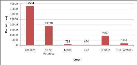
Figure 1.2: Crop
production in Gisagara district
Source: Republic of Rwanda (2006), season
statistics 2006B.
There are perhaps factors that may be hindering efficient
maize production in Gisagara district. It has been presumed that poor land use
and management practices (especially land fragmentation) in highly populated
areas can lead to inefficiencies in crop production (Gebeyehu, 1995). Gisagara
district has a very high population and land fragmentation is so common
(Musahara, 2006).
The Rwandan government believes that the cultivation of small
fragmented land holdings leads to inefficiencies in agricultural production.
Consequently, land reform programs have been introduced and generally include
the land law (passed in 2005), the land policy (adopted in 2004) and the
villagization policy (the setting up of communal settlements aimed at freeing
more land for agriculture). These land reforms strongly encourage land
consolidation (Republic of Rwanda, 2004). Under article 20 of the new land law,
farmers will have to consolidate their land and/or not fragment land holdings
below one hectare since it is argued that to be economically productive, a
household farm must not be less than 0.9 hectare, a limit set by the Food and
Agricultural Organization, FAO (Mosley, 2004). However, the Rwandan government
adopted the land reform programs without carrying out a study to assess the
effects of land fragmentation on the productivity and efficiency of farms.
It is not yet clear whether such land reforms will
successfully replace the informal rules (especially the customary land tenure
system) that encouraged land inheritance and continuous subdivision of farms.
Secondly, it is hard to predict that farmers will adopt land consolidation
especially because previous studies in Rwanda confirmed that land consolidation
does not necessarily lead to efficient crop production (
Blarel
Benoit,
Peter
Hazell,
Frank
Place and
John
Quiggin, 1992) and land fragmentation was used by farmers as a coping
mechanism to deal with problems related to land scarcity and to benefit from
regional agro-climatic differences (Marara and Takeuchi, 2003).
Production efficiency studies normally hypothesize that
technical inefficiency is influenced by farm-specific and household-specific
characteristics. The focus of this study was to especially determine whether
farm specific characteristics (with a particular focus on land fragmentation)
have negative effects on maize production in Gisagara district. Maize was
chosen because it is the most important food crop in Rwanda. Since previous
studies reported the existence of higher fragmentation levels in Gisagara
district (Musahara, 2006), Gisagara was chosen as a case study.
1.2 Statement of the
problem
The efficiency of smallholder farms in Rwanda is highly
disputed. Several factors, mainly farm-specific and household-specific
characteristics (such as education levels, dependency ratio, access to
extension services, possession of land titles among others), can reduce the
technical efficiency of farms. This study has a particular focus on the effects
of land fragmentation on the productivity and efficiency of farms.
Cultivated land in Rwanda is still small compared to total
agricultural land. This implies that land scarcity is not so extreme. There
have been claims that land fragmentation results from extreme land scarcity and
insufficiency of agricultural land (Mosley, 2004). Agricultural land during
2000-2007 was fixed at 2,294,380 hectares and there has always been a big gap
between agricultural land and cultivated land, the latter being always smaller
relative to the former. From 2000 to 2007, cultivated land has not reached
1,000,000 ha (Figure 1.3).
Figure 1.3: Cultivated land in Rwanda (`000
hectares)
Source: Republic of Rwanda (2008), Rwanda in
Statistics and Figures
The problem therefore is not that less land is allocated to
crop production but the land allocated to crop production is not efficiently
used due to practices like land fragmentation.
Farms in Rwanda have over the past been shrinking in size.
Land inheritance is common in Rwanda (Bizimana et al., 2004) and has led to
continuous subdivision of farms, leading to a fall in average farm size (Mpyisi
et al., 2003). In this study plot size, number of plots per household and
distance from the households' residences to plots were used as measures of land
fragmentation.
By 2002, only 27.1% of Rwandans had farms greater or equal to
1 hectare, but 72.9% had farms that were less than 1 ha (Table 1.4). Therefore,
land fragmentation, measured in terms of farm size, was high.
Table 1.3: Farm size distribution in 1984 and
2002
|
Farm size (ha)
|
Households
|
|
|
Percentage in 1984
|
Percentage in 2002
|
|
< 0.25
|
7.4
|
16.8
|
|
0.25-0.5
|
19
|
26.4
|
|
0.5-1.0
|
30.4
|
29.7
|
|
1.0-2.0
|
26.7
|
19.5
|
|
> 2
|
16.4
|
7.6
|
|
Total
|
99.90%
|
100%
|
Source: (Mpyisi et al., 2003).
In 2006, 93.6% of Rwandans had farms of 0.5 hectare or
less and only 6.4% of Rwandans had farms of more than 0.5 hectare (Table 1.5).
This again shows that land fragmentation, measured in terms of farm size, was
high.
Table 1.4: Farm
size distribution in 2006
|
Farm size (ha)
|
Percentage
|
|
0.25
|
61.3
|
|
0.26-0.5
|
32.3
|
|
0.51-0.75
|
1.6
|
|
0.76-1
|
3.2
|
|
1
|
1.6
|
|
Total
|
100
|
Source: Republic of Rwanda (2006), Rwanda
Development Indicators
Average farm size decreased from 1.2 ha in 1984 to
0.84 ha in 2002. In 2006, average farm size in Rwanda dropped to 0.72 ha (Table
1.6). An economically productive farm must not be less than 0.9 ha (Kelly and
Murekezi, 2000; Mosley, 2004), which is unattainable to many Rwandans.
Table 1.5: Change
in average farm size (1984-2006)
|
Average Farm size in Rwanda (ha)
|
|
Year
|
1984
|
2002
|
2006
|
|
Average farm size
|
1.2
|
0.84
|
0.72
|
Source: (Mpyisi et al., 2003) and Republic of
Rwanda (2006), Rwanda Development Indicators
In terms of geographical dispersion, Rwandans can have up to 5
plots in different locations and a household can have ten plots on average
(Musahara, 2006). The most common problems of land fragmentation include the
fact that it makes supervision and protection of land difficult; it entails
long distances, loss of working hours, the problem of transporting agricultural
implements and products; and results in small and uneconomic size of
operational holdings (Webster and Wilson, 1980).
However, land fragmentation may also be beneficial to farmers.
Bentley (1987) argued that land fragmentation may enable risk management
through the use of multiple agro-climatic zones and the practice of crop
scheduling. Growing crops in different locations may reduce the risk of losing
output due to perils such as floods, fires and destruction of crops by herds.
Land fragmentation may also enable the growing of a variety of crops that
mature and ripen at different times thereby allowing concentration of labor on
different farms at different times (Shuhao, 2005). In Rwanda, some previous
empirical studies reported that land fragmentation does not necessarily lead to
inefficiency in crop production (
Blarel
Benoit,
Peter
Hazell,
Frank
Place and
John
Quiggin1992) and that farmers used fragmentation as a coping mechanism
to deal with problems of land scarcity and to capture advantages of regional
agro-climatic differences (Marara and Takeuchi, 2003).
Previous studies in Rwanda about land fragmentation had mixed
results. The relationship between fragmentation and land productivity might not
necessarily be negative (as noted, for Rwanda, by
Blarel
Benoit,
Peter
Hazell,
Frank
Place and
John
Quiggin, 1992; Marara and Takeuchi, 2003). However, a study by Bizimana
et al. (2004) in the former Rusatira and Muyira districts of the former Butare
province revealed that the number of plots per household negatively affected
economic efficiency while plot size positively affected economic efficiency.
The authors recommended that land consolidation be adopted as it could help
increase the economic efficiency of farms. These studies however did not
capture the various dimensions of land fragmentation (plot size, distance to
the plot and number of plots per household).
This study applied the stochastic production frontier approach
(since it accounts for both measurement errors and stochastic noise) to model
the effects of each form/indicator of land fragmentation on the technical
efficiency of smallholder maize farms in Southern Rwanda using Gisagara
district as a case study.
1.3 Objectives of the
study
1.3.1 General objective
The main objective of this study was to determine the effect
of land fragmentation on the productivity and technical efficiency of
smallholder farms in Rwanda
1.3.2 Specific objectives
· To characterize smallholder maize farms in Southern
Rwanda
· To assess the levels of productivity and technical
efficiency of smallholder maize farms in Southern Rwanda
· To determine the effect of various indicators/measures
of land fragmentation on the productivity and technical efficiency of
smallholder maize farms in Southern Rwanda
1.4 Hypotheses tested
This study tested the following hypotheses:
1. Smallholder maize farms in Southern Rwanda are technically
efficient
2. Distance from households' residences to plots negatively
affects the productivity and technical efficiency of smallholder maize farms in
Southern Rwanda
3. The smaller the plot size the lower the levels of
productivity and technical efficiency of smallholder maize farms in Southern
Rwanda
4. The higher the number of plots owned by the household, the
lower the levels of productivity and technical efficiency of smallholder maize
farms in Southern Rwanda
5. Number of plots, distance to the plots and plot size reduce
the productivity and technical efficiency of smallholder farms in Southern
Rwanda
1.5 Justification of the
study
This study came at a time when the efficiency of smallholder
family farms is highly disputed in Rwanda. There was need to establish whether
smallholder farms are efficient and if not to identify the causes/sources of
such inefficiency such that appropriate policies can be adopted to address the
problem. The findings of this study will suggest key factors that may enhance
the productivity and technical efficiency of farms. Unlike previous studies in
Rwanda, this study captured plot size, distance from household residence to
plots and number of plots per household in the analysis of the effect of land
fragmentation on the productivity and technical efficiency of smallholder maize
farms in Rwanda.
2.0 ANALYTICAL FRAMEWORK AND
LITERATURE REVIEW
2.1 Analytical
framework
2.1.1 Land fragmentation
definition
McPherson (1982) argues that «when a number of
non-contiguous owned or leased farms (or `plots') of land are farmed as a
single production unit, land fragmentation exists». This means that the
plots in a farm are spatially separate. Schultz (1953) defines fragmentation as
a «misallocation of the existing stock of agricultural land.» He
points out that a fragmented farm is «...a farm consisting of two or more
plots of land so located one to another that it is not possible to operate the
particular farm and other such farms as efficiently as would be the case if the
plots were reorganized and recombined». Schultz sees land fragmentation as
a source of inefficiency.
Dovring et al. (1960) regards land fragmentation as «the
division of land into a great number of distinct plots...» when he
analyzes land reform in Europe. He points out that the French used two concepts
for land fragmentation in their consolidation operation: «îlot
de propriété» and «plotle»
(McPherson, 1982). The former referred to a piece of land owned by a single
person and surrounded by the property of others. The latter was a plot located
apart from the îlot de propriété. Land
fragmentation meant that farmers owned plotles which did not form part
of their îlots de propriété.
Papageorgiou (1963) emphasizes the role of distance in
fragmentation. He notes that fragmentation means a holding consisting of
several scattered plots over a wide area. Agarwal (1972), defines land
fragmentation as a decrease in the average size of farm holdings; an increase
in the scattering of each farmer's land; and a decrease in the size of the
individual plots in a farm holding. Binns (1950) sees fragmentation as
«...a stage in the evolution of the agricultural holding in which a single
farm consists of numerous discrete plots, often scattered over a wide
area». According to Binns' definition, land fragmentation represents a
stage in agricultural holding's evolution. This suggests that if the holding is
evolving towards consolidation, land fragmentation may be a temporary
phenomenon.
Generally, even though land fragmentation is defined in
different ways, three distinct interpretations can be identified: (1) it
implies the subdivision of farm property into undersized units that are too
small for rational cultivation; (2) it suggests that the plots are
noncontiguous and are intermixed with plots operated by other farmers; and (3)
the last type sees distance as an important aspect of land fragmentation.
2.1.2 Causes of land fragmentation
In the literature, researchers have classified the causes of
land fragmentation under two broad categories. These are supply-side causes and
demand-side causes (
Blarel
Benoit,
Peter
Hazell,
Frank
Place and
John
Quiggin, 1992; Mc Pherson 1982; Bentley 1987).
2.1.2.1 Supply-side causes of land fragmentation
Proponents of these causes assume that land fragmentation is
an exogenous imposition on farmers. Farmers involuntarily accept to hold many
plots of land, which are often dispersed. It is also assumed that fragmentation
has adverse effects on agriculture, thus farmers cannot freely choose to
scatter their land holdings unless otherwise compelled by some other forces.
These forces are reviewed in the proceeding paragraphs.
Land inheritance leads to land fragmentation when farmers
desire to provide each of several heirs with land of similar quality.
Fragmentation goes on increasing through the activity of succession from one
generation to another as parents continue to bequeath land to their children.
Extreme land scarcity also leads to land fragmentation as farmers in quest of
additional land tend to accept any available plot of land within a reasonable
distance of their house. When population pressure on land is high and when
there are no other off-farm activities upon which the population can earn a
living, fragmentation results.
Nature itself may force farmers to own scattered land holdings
in a sense that geographical barriers such as waterways and wastelands limit
the possibilities for land consolidation. Expansion of the farm under such
circumstances requires acquisition of new separate pieces of land which when
done, implies land fragmentation. Lastly, egalitarian objectives and state laws
may limit possibilities for land consolidation. For example, in China during
the 1970s and 1980s, community leaders carried out land redistribution based on
equality. Arable land was divided into a number of plots with respect to
quality and each household was given a plot (Nguyen et al. 1996). In this case,
the land redistribution process led to land fragmentation especially at the
village level.
The supply-side causes of land fragmentation explain why a
young farmer might begin with a fragmented holding. However, they do not
explain the persistence of fragmentation in face of economic incentives for
land consolidation. Such persistence indicates that there are other causes of
land fragmentation. Supply-side causes of land fragmentation have been
criticised due to many reasons.
Firstly, even when land markets afford farmers opportunities
for consolidation, fragmentation persists. This persistence implies that the
choice to own many plots of land is not always an involuntary one as assumed by
proponents of the supply-side causes of land fragmentation.
Secondly, land fragmentation has developed in areas where
there is no serious land scarcity, such as in Kenya, Zambia and Gambia (Mc
Pherson 1982). Parents continue to bestow their heirs with scattered holdings,
a practice that would seemingly be halted if land fragmentation was largely
detrimental (Leach 1968).
The argument that land inheritance is designed for equity
reasons runs into difficulty when it is observed that sub-division and
fragmentation levels are eventually «checked» after reaching certain
levels since it becomes practically impossible to continue subdividing very
tiny plots, as noted in Mexico (Downing 1977) and in Sri Lanka (Leach 1968).
The criticisms raised above suggest that supply-side causes
are not sufficient to explain the existence and persistence of land
fragmentation. It is upon this that researchers have conceived demand-side
causes of land fragmentation.
2.1.2.2 Demand-side causes of land fragmentation
The proponents of these causes view land fragmentation as a
choice variable for farmers. It is presumed that farmers will, given free
choice, choose levels of fragmentation that are beneficial to them (optimal
fragmentation). Here, farmers believe that fragmentation will bring greater
benefits to them compared to costs they are likely to incur. The demand-side
causes of land fragmentation are discussed in the proceeding paragraphs.
It is believed that land is not homogeneous with respect to
soil type, water retention capability, slope, altitude and agro-climatic
location. Farmers will freely choose to operate many plots in different
locations to enable them reduce variance in total output and hence final
consumption. Scattering of plots reduces the risk of total loss of output due
to perils such as floods, fires and droughts, which are so common in Africa
(Buck 1964; Johnson and Barlowe 1954). Scattering of plots also enables farmers
to diversify their cropping mixtures across different growing conditions
(Netting 1972).
When transaction costs in the labour market are high, farmers
will choose to scatter plots so as to better fulfil their seasonal labour
requirements and consequently obtain higher yields. If the labour market is not
working at all, labour supply is fixed by household size. Even if labour
markets exist, the costs of supervision may induce farmers to scatter their
plots and supervise a small number of workers at a time, rather than watch over
a large number of hired workers on a consolidated land holding at peak periods.
This approach is most effective when different types of land are used for
different crops (hence, when fragmentation facilitates diversification) or when
different plots of land offer sufficient diversity in climatic conditions that
the same crop can be staggered over a wide range of planting dates.
When there are commodity market failures, farmers may choose a
subsistence mode in which several products are raised for household
consumption, rather than purchased with proceeds of cash crop sales. This seems
most likely to happen when there is uncertainty about relative price movements,
especially for important foods such that trade within a village or across
villages is costly. Under this case, farmers will prefer to grow each crop on a
separate plot of land. Farmers might also want fragmented land holdings if,
holding farm size constant, there are diseconomies of scale with respect to
individual farm size. When this phenomenon occurs, however, it probably
reflects the malfunctioning of labour markets; farmers are unable to procure
adequate labour to meet seasonal peaks in the requirements for large farms.
It is quite clear that demand-side causes of land
fragmentation consider fragmentation as a deliberate choice made by farmers so
as to reduce risks associated with crop production; this is why scholars have
deemed it «fragmentation for risk reduction». Critics of demand-side
causes of fragmentation assert that it should only persist if other
risk-reduction mechanisms, such as insurance, storage or credit, are either not
available or more costly (Hyodo 1963; Ilbery 1984; Thompson 1963). The flaws
seen in both supply-side and demand-side causes suggest that each side of these
causes should complement the other in providing explanations for the occurrence
and persistence of land fragmentation.
2.1.3 Effects of land
fragmentation
Land fragmentation has both advantages and disadvantages and
the debate about which side outweighs the other seems to be a perpetual one.
The advantages of land fragmentation are similar to the demand side causes of
land fragmentation.
2.1.3.1 Disadvantages or costs of land fragmentation
The costs of land fragmentation are quite many. In this study,
the costs of land fragmentation considered are discussed in Shuhao (2005) and
Raghbendra (2005). These costs are reviewed in the paragraphs below.
Land fragmentation leads to increased travelling time between
fields, hence lower labour productivity and higher transport costs for inputs
and outputs. Fragmentation also involves negative externalities such as reduced
scope for irrigation, soil conservation investments and loss of land for
boundaries and access routes. Farmers may also incur higher costs of
supervising workers on each separate farm than when supervision occurred on a
large farm.
Fragmentation also involves greater potential for disputes
between neighbours. These conflicts arise when farmers do not agree with the
current farm demarcations especially because they believe that their neighbours
have cheated them by taking some land from their respective farms. Lastly,
farmers owning scattered plots that are quite far away from their homes may
lose output due to perils such as destruction of crops by herds, fires, floods,
thefty and droughts.
Causes of land fragmentation in Rwanda
The major cause of land
fragmentation in Rwanda over the past has been population pressure on land (a
supply side cause). Due to population pressure, land has been so scarce that
people resorted to purchasing and renting of land and even migrations.
In the 1960s, some researchers had
started warning of a growing land scarcity in Rwanda. Landal (1970) stated that
« it is assumed that by 1975 ceteris paribus, there will be no further
land for cultivation lying idle». This became a reality in the 1980s when
several Rwandan families started migrating into countries neighbouring Rwanda
because they could not get any land for cultivation. There were also internal
migrations whereby people moved from areas of high population pressure to areas
of low population pressure. Bugesera region, whose population density was 20
persons per square kilometre in 1960 and rose to 120 persons per square
kilometre in 1978, is a good example (Clay and Ngenzi 1990).
Indeed, land inheritance has
existed in Rwanda for so long. Recently, it has been sons and not daughters who
customarily inherit land. However, some traditions enabled women to inherit
land. These included Urwibutso; a tradition by which
a father would give land to a daughter as a gift,
Inkuri; a tradition by which a father would give land
to his daughter as a gift when she gave birth (common in Ruhengeri),
Intekeshwa; a tradition by which a father gave land
to the daughter as a farewell gift upon getting married and finally,
Ingaligali; a tradition by which a land chief would
give land to women who were abandoned by their spouses. All these led to land
fragmentation (Musahara 2006). Currently, laws have been made to incorporate
the issue of gender equity in issues related to inheritance of property.
Demographic pressure on land in Rwanda
According to Rwanda Development
Indicators (RoR 2003), Rwanda remains one of Africa's most densely populated
countries, with more than 340 inhabitants per square kilometre. The rate of
population growth was estimated at 3.1% in 1998. It is projected that Rwanda's
population will double over the next twenty years; from 8.2 million inhabitants
to at least 16 million inhabitants. Population density will certainly rise to
865 inhabitants per arable square kilometre.
In the last 50 years, the
population of Rwanda has almost quadrupled. The population in 1934 was just
over one and a half million. It had risen to 8.16 million in 2003. Some 40
years ago, density on arable land was 121 persons per square kilometre; the
figure rose to 166 persons per square kilometre in ten years later, it is
thought to have been approximately 262 persons per square kilometre in 1990;
and by 1999, it was well above 350 persons per square kilometre (Baechler
1999). There is thus considerable pressure on land (a fixed factor), and this
has made population pressure one of Rwanda's major challenges.
Another important characteristic
of the Rwandan population is that a majority of this population lives in rural
areas. This rural population largely depends on farming. As population grows
rapidly, land becomes scarce. Farmers resort to purchasing and renting of land.
Indeed, family planning practices have not been successful in Rwanda; a family
produces many children who, after growing up are bequeathed with a portion of
land and this leads to land fragmentation.
Impact of population pressure on land distribution in
Rwanda
In Rwanda, population pressure on
land has resulted into continuous fall in farm size. Table 2.1 highlights the
changes in farm holdings that took place between 1984 and 2002.
Table .1: Distribution of land owned at the
household level in Rwanda by farm size
Farm size Classification by Area
Owned
|
Households
|
Total land owned
|
% in 1984
|
% in 2002
|
% in 1984
|
% in 2002
|
Less than 0.25 ha
|
7.4
|
16.8
|
1.0
|
3.3
|
0.25-0.5 ha
|
19.0
|
26.4
|
5.9
|
11.8
|
0.5-1.0 ha
|
30.4
|
29.7
|
18.4
|
25.4
|
1.0-2.0 ha
|
26.7
|
19.5
|
31.8
|
31.7
|
Greater than 2 ha
|
16.4
|
7.6
|
42.9
|
27.8
|
Total
|
99.9%
|
100%
|
99.7%
|
100%
|
Average farm size in Rwanda in ha
per household
|
# Rural households 1,111,897
|
# Rural Households 1,442,681
|
1.2 ha
|
0.84 ha
|
Source: Mpyisi E.
et al. (2003). Note: The symbol # in table 2.1 means «Total number
of».
In 1984, some 43.1 % of rural
households had farms of 1 hectare and larger. These farms occupied 74.7 % of
the total land owned. In 1984 some 16.4 % of households had farms greater than
2 hectares, and this group occupied 42.9 per cent of land.
By 2002, the percentage of
households with farms of 1 hectare or larger had dropped to 27.1% but this
group still occupied almost 60 percent of land. The percentage of households
with less than 0.5 hectares increased from 26.4 % in 1982 to 43.2 % in 2002,
but as a group these farms only occupied about 15.1 % of land. The average farm
size decreased from 1.2 ha in 1984 to 0.84 ha in 2002.
2.1.4 Technical efficiency
definition and measurement
According to Farrell (1957), technical efficiency reflects the
firm's ability to maximize the output for a given set of inputs (operate at the
boundary of a production possibility frontier), or the firm's ability to
minimize inputs used for a given set of output. The measurement of technical
(in) efficiency can be classified into two categories: input-orientated
measures and output-orientated measures. This study applied the
output-orientated measure but reviewed literature about the two measures.
2.1.4.1 Input-orientated
measure of technical efficiency
The input-orientated measure of technical efficiency seeks to
answer the question: «By how much can input quantities be proportionally
reduced without changing the output quantities produced?» Farrell (1957)
illustrated the definition of the input-orientated measure of technical
efficiency using a simple example involving firms, which use 2 inputs (x1 and
x2) to produce a single output (y), under the assumption of constant returns to
scale (to enable the representation of the production technology on a single
isoquant). Knowledge of the unit isoquant (represented by the line SS' in
figure 2.1) of the fully efficient firm permits the measurement of technical
efficiency.
If a given firm uses quantities of inputs defined by point P
to produce a unit of output, the technical inefficiency of that firm could be
represented by the distance QP which is the amount by which all inputs could be
proportionally reduced without a reduction in output. This is usually expressed
in percentage terms by the ratio which represents the percentage by which all
inputs could be reduced, keeping output constant. The technical efficiency of a
firm is most commonly measured by the ratio which is equal to . Technical
efficiency takes on either 1 or 0 or values between 1 and 0 and hence provides
an indicator of the degree of the technical inefficiency of a firm. A value of
1 indicates that the firm is fully technically efficient while the value of 0
indicates that the firm is fully technically inefficient. For example the point
Q is technically efficient because it lies on the efficient isoquant.
A S P
Q
R
Q'
S'
0 A'
x1/y
Figure .1:
Technical efficiency and allocative efficiency under input-orientated
measure
If the input price ratio represented by the line AA' is also
known, allocative efficiency of the firm can also be calculated. Allocative
efficiency of the firm operating at point P is defined as
. The distance RQ represents the reduction in production costs
that would occur if production were to occur at the allocatively (and
technically) efficient point Q' instead of the technically efficient but
allocatively inefficient point, Q. The total economic efficiency is defined to
be the ratio where the distance RP can also be interpreted in terms of a cost
reduction. Note that the product of technical efficiency (TE) and allocative
efficiency (AE) provides the overall economic efficiency (EE). That is EEI= TEI
OR/OQ = OR/OP. Note also that TE, AE and EE are bounded by 0 and 1.
The efficiency measures explained above assume that the
production function of a fully efficient firm is known. In practice this is not
the case, and the efficient isoquant must be estimated from the sample data.
Farrell (1957) suggested the use of (a) a non-parametric piecewise-linear
convex isoquant constructed such that no observed point lies to the left or
below it as shown in figure 2.2, and (b) a parametric function such as the
Cobb-Douglas production function, fitted to the data, again such that no
observed point should lie to the left or below it.
x2/y S
.
.
.
S'
O
x1/y
Figure 2.2: Piece wise linear convex
isoquant
2.1.4.2 Output-orientated
measure of technical efficiency
This addresses the question: «by how much can output
quantities be proportionally expanded without altering the input quantities
used?» This can be illustrated using a decreasing returns to scale (DRS)
technology represented by f(x) and an inefficient firm operating at P.
y
D f(x)
A B P
O C
x
Figure 2.3: Decreasing Returns to Scale
(DRS)
The Farrell input-orientated measure of technical efficiency
would be AB/AP while the output-orientated measure would be CP/CD. The two
measures of technical efficiency can only be equal if constant returns to scale
(CRS) exist but will be unequal if both increasing returns to scale (IRS) and
decreasing returns to scale (DRS) exist. The CRS case is presented in figure
2.4 below:
f (x)
y D
A B P
O C
x
Figure 2.4: Constant Returns to Scale (CRS)
case
In the CRS case, we observe that for any inefficient point P
we may choose. One can consider the output-orientated measure of technical
efficiency further by considering a case where production involves 2 outputs
(y1 and y2) and a single input (x). Again if we assume CRS, we can represent
the technology by a unit production possibility curve in 2 dimensions. This
example is illustrated in figure 2.5 below.
y2/x
D
C
Z B B'
.A
D'
O
Z' y1/x
Figure 2.5: Technical efficiency (TE) and
allocative efficiency (AE) from output-orientation
The line ZZ' is the unit production possibility curve. The
distance AB represents technical inefficiency (TIE). That is, the amount by
which outputs could be increased without requiring extra inputs, hence a
measure of output-orientated efficiency is: . If we have price-information,
then we can draw the isorevenue line DD' and define allocative efficiency (AE)
to be: AE0 = OB'/OA which has a revenue increasing interpretation. Further,
one can define the overall economic efficiency (EE) as the product of these 2
measures:
EE0 = OB'/OB = TE0 AE0 = OA/OB OB'/OA. Again, all the 3
measures are bound by 0 and 1. Note that point C is unattainable at the current
level of technology.
2.2 Literature review
2.2.1 Effect of land
fragmentation on the productivity and technical efficiency of farms
The literature on land size and land productivity is large and
has been around for decades. In recent times Binswanger et. al. (1995) argued
that there was an inverse relationship between the two whereas Banerjee and
Ghatak (1996) questioned this result. Carlyle (1983), Heston and Kumar (1983),
Bentley (1987),
Blarel
Benoit,
Peter
Hazell,
Frank
Place and
John
Quiggin, (1992), Jabarin and Epplin (1994) focused on the impact of
fragmentation on yield and productivity. The debate basically focused on the
impact of fragmentation on the ability of farmers to minimize risk. These
studies perceived land fragmentation to have a negative impact on productivity
and yield.
The countries where the relationship between land size and
technical efficiency has been studied include the Philippines (Herdt and Mandac
1981; Dawson and Linagard 1989), Brazil (Taylor and Shonkwiler 1986), Tanzania
(Shapiro 1983), Pakistan (Ali and Chaudhry 1989) and India (Huang and Bagi
1984; Kalirajan 1981; Junankar 1980; Sidhu 1974; Lau and Yotopoulos 1971;
Battese, Coelli and Colby 1989; Tadesse and Krishnamoorthy 1997).
The studies used the stochastic production function approach and
concluded that the large variation in yield across farmers was due to
differences in technical efficiency, which was largely influenced by farm size
and ecological and socio-economic factors such as gender, age, education,
extension services, access to credit, among others.
Raghbendra et al. (2005) investigated the impact of land
fragmentation on technical efficiency of rice farms in India using the
stochastic frontier method and confirmed that there was a significant positive
relationship between farm size, average farm size and yield while the number of
plots and yield were inversely related. Therefore fragmentation measured in
terms of number of farms per household had a negative impact on yield.
Shuhao (2005), using the stochastic frontier method,
investigated the impact of land fragmentation on rice production in China and
found out that land fragmentation played an important role in explaining
technical efficiency. Given the number of plots, increase in average plot size
had a significant positive impact on technical efficiency. Distance to the
plots, however, had no significant impact on technical efficiency. This implied
that farm households with large average distances to the plots were as
efficient as farm households with small average distances to the plots.
Bizimana et al. (2004) used a block-recursive regression analysis to
investigate the effect of land fragmentation on economic efficiency of farms in
Rwanda's Butare district. They concluded that land fragmentation reduced the
economic efficiency of farms. However, this study did not capture the various
dimensions of land fragmentation.
Land fragmentation and productivity/efficiency in
Rwanda
Blarel (1989) made research about the effects of land
fragmentation on the productivity of farms in Rwanda. To him, land
fragmentation has no negative effect on the productivity and efficiency of
farms. He argued that farmers operating small farms intensify their farm
operations through a more rigorous use of available family labor, a
substitution toward higher yielding crops, sowing seeds more densely and
growing more crops in associations. Small farms also benefited much from
conservation investments such as terraces, living fences, and mulching. He
discussed other determinants of productivity/efficiency of farms and concluded
that Rwandan farmers were far more likely to invest in the fields for which
they had land titles than in fields rented from others. Indeed, higher yields
occurred on parcels operated under short-term use rights than under ownership
rights.
Blarel
Benoit,
Peter
Hazell,
Frank
Place and
John
Quiggin (1992) found out that 40% of Rwandan households owned 8 or more
parcels. They still concluded that land fragmentation seemed to have a negative
effect on the productivity and efficiency of farms. Place and Hazzel (1993)
confirmed that peasants make long-term investments (planting trees, trenching,
de-stumping, and green fencing) and short-term investments (continued mulching
and manuring) in land if they had secure long-term ownership rights on that
land. But these investments do not guarantee that output will be high since
other factors such as technology and availability of financial credit affect
productivity and efficiency.
Byiringiro and Reardon (1996) found out that farm size and
productivity/efficiency were inversely related whereas farm size and labor
productivity were positively related. To them, small farms invest twice as much
per hectare in soil conservation compared to large farms. They however,
discovered that soil erosion severely reduces farm yields in Rwanda.
Studies carried out in Southern Rwanda revealed that the
relationship between fragmentation and land productivity might not necessarily
be negative (
Blarel
Benoit,
Peter
Hazell,
Frank
Place and
John
Quiggin, 1992; Marara and Takeuchi, 2003). However, a study by Bizimana
et al. (2004) in the former Rusatira and Muyira districts of the former Butare
province revealed that the number of plots per household negatively affected
economic efficiency while plot size positively affected economic efficiency.
The authors recommended that land consolidation be adopted as it could help
increase the economic efficiency of farms.
However, most studies carried out in Rwanda about land
fragmentation did not capture all forms/indicators of land fragmentation.
Blarel
Benoit,
Peter
Hazell,
Frank
Place and
John
Quiggin (1992) used the Simpson index as a measure of fragmentation yet
it does not capture the effect of distance travelled to reach the plots. Marara
and Takeuchi (2003) only considered the number of plots per household while
Bizimana et al. (2004) considered plot size and number of plots per household.
This study attempted to include plot size, distance from household residence to
plots and number of plots per household in the analysis of the effect of land
fragmentation on the productivity and technical efficiency of smallholder maize
farms in Rwanda.
3.0 METHODS AND
PROCEDURES
3.1 Theoretical model
3.1.1 Indicators of land fragmentation
Different researchers have used several measurement units in
their attempt to measure land fragmentation. Common measures include the
Simpson index (SI), the Januszewski index (JI) and average farm size.
The Simpson Index (
Blarel
Benoit,
Peter
Hazell,
Frank
Place and
John
Quiggin, 1992), which is defined as:
Where n is the number of plots, and is the area of
each plot. This index is located within the range of 0 to 1. A higher SI value
corresponds with a higher degree of land fragmentation. The value of the
Simpson index is determined by the number of plots, average plot size and the
plot size distribution. It also does not take farm size, distance and plot
shape into account.
Average farm size (Nguyen et al. 1996) defined as:
Where S is the size of the farm and N is the
number of plots. When N is large, average plot size, P is small. This
implies that as fragmentation increases, average farm size reduces and
vice-versa. This measure of land fragmentation simply looks at the way in which
a farm is subdivided into a given number of plots. The drawback of using
average farm size as a measure of land fragmentation is that it only considers
subdivision of the same piece of land (farm) due to inheritance only.
The Januszewski index (Raghbendra et al. 2005) defined as:
Where n is the number of plots,
and is the area of each plot. This index is located within
the range of 0 to 1. The smaller the JI value the higher degree of land
fragmentation. The JI value combines information on the number of plots,
average plot size and the size distribution of the plots. It has three
properties: fragmentation increases (the value of the index decreases) when the
number of plots increases, fragmentation increases when the average plot size
declines, and fragmentation decreases when the inequality in plot sizes
increases. The index, however, fails to account for farm size, plot distance,
and shape of plots.
Single-dimension
indicators of land fragmentation (Shuhao, 2005):
There are three indicators/measures of land fragmentation; (1) plot
size, (2) number of plots per household and, (3) the distance from household
residences to plots. This study used these three measures of land fragmentation
because we wanted to capture explicit effects of each single-dimension
indicator on the productivity and technical efficiency of farms.
3.1.2 Measuring technical
efficiency
Choosing between a parametric (stochastic frontier model) and
a non-parametric (Data Envelopment Analysis) approach to measure efficiency has
been controversial. Each has its strengths and weaknesses (Coelli and Perelman,
1999). The parametric analysis deals with stochastic noise, and allows
hypothesis testing on production structure and efficiency. However, this method
has to specify a functional form for the production frontier and imposes a
distributional assumption on the efficiency term. The non-parametric method
does not impose such restrictions, but it assumes the absence of measurement or
sampling error. The choice between these approaches, therefore, depends upon
the objective of the research, the type of farms that are analyzed, and data
availability.
The stochastic frontier method has been used for both
cross-sectional and panel data. In Tanzania, Mbelle and Sterner, (1991) applied
the model to analyze the importance of foreign exchange in industries. Other
studies include among others, those of Battese and Coelli (1995); Raghbendra et
al (2005); Hyuha et al. (2008) and Bagamba (2007).
This study used the stochastic frontier approach - a
parametric method - to analyze the effect of land fragmentation on the
technical efficiency of smallholder maize farms in Southern Rwanda. The main
reason for this choice is that maize production in Rwanda is subject to weather
disturbances and heterogeneous environmental factors like soil quality.
Moreover, the respondents might not always answer all the questions precisely,
due to for example having varied perceptions, and this will affect measured
efficiency (Chen et al., 2003).
3.2 Theoretical
considerations
There are two approaches used to estimate technical
efficiency: the one-step approach and the two-step approach. The two-step
procedure using the stochastic frontier production function generally involves
first estimating the production frontier then predicting the technical
efficiency of each firm. In the second step, the predicted technical efficiency
variable is regressed against a set of variables that are hypothesized to
influence the firm's efficiency (Kalirajan, 1981).
However, the two-stage procedure lacks consistency in
assumptions about the distribution of the inefficiencies. In step one, it is
assumed that inefficiencies are independently and identically distributed in
order to estimate their values. In step two, estimated inefficiencies are
assumed to be a function of a number of firm-specific factors, violating this
assumption (Coelli, 1996). To overcome this inconsistency, Kumbhakar et al.
(1991) suggest estimating all the parameters in one step. In the one-step
procedure, the inefficiency effects are defined as a function of the
farm-specific factors and incorporated directly into the maximum likelihood
(ML) estimate. This study used the single-step procedure.
In this study, a farm specific stochastic production frontier
involving outputs and inputs was defined as follows:
................................................. (1)
Where is the maximum possible stochastic potential output
from the ith farm; is a vector of m inputs and are statistical
random errors assumed to be distributed as . The production realized on the
ith farm can be modeled as follows:
............................................ (2)
Where is defined as a measure of observed TE of the
ith farm assuming that = 0. When takes the value zero, the
ith farm is technically efficient and realizes its maximum possible
potential output. Thus TE can be defined as a ratio between the firm's realized
output and the firm's stochastic/potential output as shown in equation 3:
............................................... (3)
Substituting equation (1) into equation (2) and taking logs on
both sides gives:
....................................... (4)
Where denotes the production of the ith farm (i =
1, 2,..., n); is a (1 x k) vector of functions of input quantities used by the
ith farm; â is a (k x 1) vector of unknown parameters to be
estimated; are random errors assumed to be independently and identically
distributed with and they are independent of the . The is a one-sided error
term representing the technical inefficiency (TIE) of farm i.
Subtracting from both sides of equation (4), the production
of the ith farm can be estimated as:
...................................... (5)
Where is the natural logarithm of the predicted output of the
ith farm, is the natural logarithm of the ith input is a
set of parameters and is the measure of observed technical efficiency of the
ith farm.
Define the efficient level of production as:
................................................ (6)
Where is the natural logarithm of the output of the
technically efficient farm, is the natural logarithm of the ith
input and is a set of parameters.
Then, from equations (5) and (6), computation of technical
efficiency (TE) is given in equation 7:
or equivalently, ................................ (7)
Arguments in equation 7 are defined in equations 5 and 6. From
equation 7, it follows that and when, then = 1 and production is said to be
technically efficient.
The distribution of could be half normal with zero mean,
truncated normal (at mean, ì), or based on conditional expectation of
the exponential (). There are no a priori reasons for choosing a specific
distributional form of because each has advantages and disadvantages (Kebede,
2001). The half normal and exponential distributions have a mode of zero,
implying that most firms being analyzed are efficient. The truncated normal
allows for a wide range of distributional shapes, including non-zero modes, but
is computationally more complex (Coelli, 1996).
This study used the technical inefficiency model proposed by
Battese and Coelli (1995), and defined the technical inefficiency effects as
follows:
............................................................
(8)
Where is a (1 x m) vector of explanatory variables associated
with the technical inefficiency effects; ä is an (m x 1) vector of unknown
parameters to be estimated; and are unobservable random variables. The
parameters indicate the impacts of variables in z on technical inefficiency.
The frontier model may include intercept parameters in both the frontier and
the model for the inefficiency effects, provided the inefficiency effects are
stochastic and not merely a deterministic function of relevant explanatory
variables (Battese and Coelli, 1995).
Battese and Corra (1977) parameterised the variance terms of u
and v as:
and ................................. (9)
Where is the variance of output conditioned on inputs. This
says that the production uncertainty comes from two sources: pure random
factors and technical inefficiency. Hence if , the proportion of uncertainty
coming from technical inefficiency, is equal to zero, then it actually means
there is no technical inefficiency. This can be used to test whether technical
inefficiency is present in the firm. Further, the null hypothesis that the
impact of the variables included in the inefficiency effects model in equation
(8) on the TIE effects is zero is expressed by H0: ä ? = 0 , where ä
? denotes the vector, ä , with the constant term, , omitted (Battese and
Broca, 1997).
3.2.1 Model specification
According to Battese and Coelli (1995), the functional form of
the stochastic production frontier needs to be specified. In practice, both the
Translog and the Cobb-Douglas forms are usually adopted. The Translog form is
more flexible in permitting substitution effects among inputs, and is claimed
to be a relatively dependable approximation to reality while the Cobb-Douglas
form is simple and commonly used.
Kopp and Smith (1980) argue that functional specification has
a discernible, though rather small, impact on estimated efficiency. Taylor
et al. (1986) also argue that as long as interest rests on efficiency
measurement and not on the analysis of the general structure of the production
technology, the Cobb-Douglas production function provides an adequate
representation of the production technology. Therefore, following Nguyen et
al. (1996), a stochastic Cobb-Douglas production function was estimated
because of its simplicity. We define the empirical form of the stochastic
production function in equation 10:
The variables included in the stochastic production model and
their expected signs are summarized in table 3.1.
Table 3.1:
Variables in the stochastic Cobb-Douglas production model
|
Variable
|
Definition
|
Measurement unit
|
Effect
|
|
Land area planted with maize in season A (September 2008-February
2009)
|
maizearea
|
Hectares
|
+
|
|
Household size in season A (September 2008-February 2009)
|
hhsize
|
Number of persons in the household
|
+
|
|
Quantity of maize seed* used for maize production in season
A(September 2008-February 2009)
|
seed
|
Kgs
|
+
|
|
Maize output in season A(September 2008-February 2009)
|
maizeout
|
Kgs
|
Dependent
|
*Maize seed includes both the improved and local varieties.
However, Rwandan farmers generally use the improved variety.
Household size was used as a proxy for labor because larger
households are always likely to have many people to participate in agriculture.
During the survey, it was found out that hired labor is not so much used.
Therefore observations with hired labor as outliers were excluded from the
sample. All inputs in the Cobb-Douglas production function are expected to
have a positive impact on maize output since an increase in each (or all of)
the inputs can lead to increased output.
The technical inefficiency (TIE) model was defined in equation
11:
................................................................. (11)
Where by is an error term which can be assumed to be
distributed as truncated normal, half normal or exponential distribution. Note
that instead of using indices (such as the Simpson index), single dimension
indicators (number of plots per household, average plot size and average
distance walked to reach a plot) were used to measure land fragmentation. This
allowed for obtaining the explicit effect of each single dimension indicator on
productivity and technical efficiency. The variables included in the technical
inefficiency model and their expected signs are summarized in table 3.2.
Table 3.2:
Variables in the technical inefficiency model
|
Variable
|
Label
|
Measurement unit
|
Expected sign
|
|
Age of household head
|
Age
|
Years
|
+/-
|
|
Education level of household head
|
education
|
Years spent in school
|
+/-
|
|
Dependency ratio
|
dependratio
|
Dependency ratio
|
+
|
|
Number of plots per household
|
noplots
|
Number of plots owned by household
|
+/-
|
|
Plot size
|
plotsize
|
Hectare
|
+/-
|
|
Average distance from plots to homestead
|
avplotdist
|
Kilometers
|
+
|
|
Number of extension visits received by household in season
A
|
Extension
|
Number of visits
|
-
|
|
Distance to the nearest market center
|
Distmkt
|
Kilometers
|
+
|
|
Dummy for land title
|
dummytitle
|
D=1 for have title, 0 otherwise
|
-
|
|
Dummy for agro-climatic zone
|
agroclimate
|
1 for Bwanamukali, 0 for Mayaga
|
-
|
|
Sex of the household head
|
Sex
|
1=Male, 0=female
|
+/-
|
|
TIE
|
Technical inefficiency
|
|
Dependent
|
Most studies have associated farmers' age and farmers'
education with technical efficiency. Farmers' age and education are reported by
many studies as having a positive effect on technical efficiency (Amos, 2007;
Ahmad et al., 2002; Kibaara, 2005). Age may have a positive effect on technical
efficiency if due to experience; older farmers tend to adopt better farming
methods than young farmers. A higher level of education can lead to a better
assessment of the importance and complexities of production decisions,
resulting in better farm management. Educated farmers learn faster and utilize
well extension information (Basnayake and Gunaratne, 2002).
In other studies the effect of age and education is ambiguous
(Shuhao, 2005). Dependency ratio is reported to have significant negative
effects on technical efficiency (Bagamba, 2007) while the farmers' gender (sex)
can have ambiguous effects on technical efficiency (Tchale and Sauer, 2007).
Although studies by Amos (2007), Raghbendra, Nagarajan and
Prasanna (2005), and Barnes (2008) found the relationship between land holding
size and efficiency to be positive, a clear-cut conclusion on the influence of
this variable on efficiency has not been reached as discussed in
Kalaitzadonakes et al (1992) work. On the other hand, effect of the number of
plots on efficiency has been hypothesized to be either negative (Raghbendra et
al, 2005) or positive (Marara and Takeuchi, 2003) or ambiguous (Shuhao, 2005).
It was hypothesized that the effect of number of plots on efficiency was
ambiguous.
Distance from plots to residence is expected to negatively
affect efficiency (Byiringiro and Reardon, 1996) Extension visits are expected
to increase efficiency and distance to the nearest market is expected to reduce
efficiency (Bagamba, 2007). Land ownership rights (possession of land titles)
has been assumed to encourage soil conservation investments and therefore
expected to increase productivity and efficiency (Musahara, 2006). This study
expected agro-climate to have a negative effect on inefficiency since
Bwanamukali is more fertile and receives more rainfall than Mayaga.
Age had been expected to have a quadratic effect on technical
efficiency. However, results showed that age and its square had the same sign
and were both not significant (once the square of age was included in the
model) but age was significant (once the square of age was excluded from the
model). Thus, the square term of age was excluded from the model.
The analysis of productivity for
several crops can be made by regressing marginal value products against
farm-specific and household specific characteristics. For a single crop,
marginal physical products can be used (Byiringiro and Reardon, 1996). This
study used marginal physical products as the dependent variable and all
dimensions of land fragmentation as the independent variables. To analyze the
productivity of smallholder maize farms, the following double-log regression
model was specified:
Where is the natural log of the marginal product of land
under maize, is the natural log of the size of the farm owned by a household,
is the natural log of the total number of plots owned by the household, is
the natural log of the average distance between households residences to plots
and is the error term that is assumed to be independently and identically
distributed with zero mean and constant variance. The interaction term was
included to show what happens when a household has many/few farms that may be
distant/close to each other.
Apriori, it was expected that farm
size is positively/negatively related to the productivity of farms as there is
mixed literature about this. Number of plots and distance between plots are
both expected to constrain productivity. The interaction between distance and
number of plots can be negative if a household has many plots that are located
far apart from each other, otherwise this interaction may have insignificant
effect as long as plots are near each other.
3.3 Data and sources
3.3.1 Study area
This study was carried out in Rwanda's Southern province,
particularly in Gisagara district. A district is an administrative unit that
comes next to the province (the highest local administrative unit) while a
sector is an administrative unit that comes next to the district. There are 13
sectors (Nyanza, Kigembe, Kansi, Kibirizi, Muganza, Mugombwa, Mukindo, Musha,
Gishubi, Mamba, Gikonko, Ndora, and Save) in Gisagara district. More
information about Gisagara district is provided in appendix 2 and appendix 3.
Gisagara district was purposively chosen because land fragmentation is so
common there (Bizimana et al., 2004 and Musahara, 2006).
3.3.2 Sampling methods
In this study, a two-stage sampling technique was used to
select the sample. Stage one involved a random selection of sectors. Out of the
13 sectors, 7 were randomly selected and these were Save, Kibirizi, Kansi,
Musha, Gikonko, Gishubi and Mamba. Simple random sampling was applied at stage
one.
A sampling frame (a list of households) was obtained for each
sector and at stage two respondents were selected from each sector using
systematic random sampling (whereby the first kth household was
selected randomly) as shown in table 3.4 below. A sample size of 280 households
was selected.
However, after excluding outliers, a sample size of 241
households remained. Primary data for this study were collected using a
structured household questionnaire (see appendix 1). The structured household
questionnaires were administered to respondents by enumerators under
supervision of the researcher. The field survey was conducted from
20th May 2009 to 25th June 2009.
Table 3.3: Systematic random sampling
procedure
|
Sector
|
Total Households ()
|
Desired Sample size (
|
th interval ()
|
|
Kibirizi
|
5530
|
40
|
138
|
|
Kansi
|
4055
|
40
|
101
|
|
Gikonko
|
4420
|
40
|
111
|
|
Gishubi
|
5084
|
40
|
127
|
|
Mamba
|
6677
|
40
|
167
|
|
Musha
|
4853
|
40
|
121
|
|
Save
|
5640
|
40
|
141
|
|
Total
|
36259
|
280
|
|
Source: the sampling frames were obtained
from each sector's official reports
3.3.3 Data analysis
Data collected were coded, entered and cleaned using the
Statistical Package for Social Scientists (SPSS) computer program. The data
were then transferred to Stata in which econometric analyses were carried out.
Diagnostic tests (to check for normality, multicollinearity and outliers) were
then carried out. As a result, 39 outliers were removed leaving a sample size
of 241 households. Descriptive statistics (percentages, means and standard
deviations) were generated.
A Cobb-Douglas stochastic production function was estimated
using the single-step procedure suggested by Kumbhakar et al. (1991) that
produces maximum likelihood estimates of the stochastic production function.
This procedure is superior to the two-stage procedure because it does not
violate the assumption that the inefficiency effects are independently and
identically distributed (Battesse and Coelli, 1995).
4.0 RESULTS AND
DISCUSSION
In this chapter the
results of the study are presented and discussed. First, we characterize
smallholder maize farms in Gisagara district and later analyze their
productivity and technical efficiency.
4.1 Characterization of
smallholder maize farms in Gisagara district
A total of 241 household
heads from Gisagara district were retained as the sample (after excluding 39
outliers). The number of households managed by males was quite higher than the
number of households managed by females (Table 4.1). This however did not
tempt us to expect that sex would have a positive effect on technical
efficiency since its effect has been reported in the literature to be ambiguous
(Tchale and Sauer, 2007).
Table 4.1: Gender decomposition of households
|
Sex of the household head
|
Frequency
|
Percentage
|
|
Female
|
102
|
42
|
|
Male
|
139
|
58
|
|
Total
|
241
|
100
|
Source: Survey data, 2009
Generally, almost 80
percent of households in Gisagara district had 30 or more years (Table 4.2).
The implication is that if old age had a significant positive effect on
technical efficiency, then a majority of households would be efficient.
However, some literature considers age to have an ambiguous effect (Shuhao,
2005).
Table 4.2: Age frequency distribution of
household heads
|
Age of household head
|
Frequency
|
Percentage
|
|
18-30
|
49
|
20.3
|
|
30-42
|
76
|
31.5
|
|
42-54
|
60
|
24.9
|
|
54-66
|
40
|
16.6
|
|
66 and above
|
16
|
6.6
|
|
Total
|
241
|
100
|
Source: Survey data,
2009
In many studies, education has been hypothesized to positively
influence technical efficiency of farms (Amos, 2007; Kibaara, 2005). Education
levels of household heads of Gisagara district were low given that those who
attained either secondary or university education were only 9.13 and 90.87
percent either had no education or attained primary education. However, almost
66 percent attained some education (Table 4.3).
Table 4.3: Distribution of
household heads according to education level
|
Education level of household head
|
Frequency
|
Percentage
|
|
No education
|
82
|
34.02
|
|
Primary
|
137
|
56.85
|
|
Secondary
|
20
|
8.30
|
|
University
|
2
|
0.83
|
|
Total
|
241
|
100
|
Source: Survey data,
2009
Households with a dependency ratio of 0.5 or larger were
almost 71 percent (Table 4.4). Since higher dependency ratio has been reported
to reduce efficiency levels (Bagamba, 2007.
Table 4.4: Dependency ratio
of household heads
|
Dependency ratio
|
Frequency
|
Percentage
|
|
0
|
26
|
10.8
|
|
0.1-0.5
|
45
|
18.7
|
|
0.5-0.9
|
155
|
64.3
|
|
1
|
15
|
6.2
|
|
Total
|
241
|
100
|
Source: Survey data,
2009
Access to extension services has been reported to positively
influence technical efficiency of farmers especially because farmers acquire
information about better farming practices and agricultural technologies
(Bagamba, 2007; Shuhao, 2005). In Gisagara district, access to extension
services was low given that only 19 percent received 1 extension visit or more
during season A of 2008/09 (Table 4.5).
Table 4.5: Extension visits
received by households
|
Extension visits
|
Frequency
|
Percentage
|
|
0
|
195
|
81
|
|
1-5
|
40
|
16.6
|
|
6-10
|
5
|
2
|
|
11-15
|
1
|
0.4
|
|
Total
|
241
|
100
|
Source:
Survey data, 2009
Possession of land titles
helps to improve land tenure security and makes land owners feel confident to
make long-term investments in their land which in turn may enhance their
productivity and technical efficiency (Blarel, 2001; Musahara, 2006). In
Gisagara district, the number of households with land titles was higher than
those without titles (Table 4.6).
Table 4.6: Possession of land titles
|
Land title
|
Frequency
|
Percentage
|
|
Have title
|
138
|
57.3
|
|
Have no title
|
103
|
42.7
|
|
Total
|
241
|
100
|
Source: Survey data, 2009
Gisagara district is divided into 2 agro-climatic zones,
Bwanamukali (which receives more rainfall and is more fertile) and Mayaga
(which receives less rainfall and is less fertile). The number of households
who belonged to Bwanamukali was higher than that of Mayaga (Table 4.7).
Table 4.7: Households per agro-climatic
zone
|
Agro-climatic zone
|
Frequency
|
Percentage
|
|
Bwanamukali
|
139
|
57.7
|
|
Mayaga
|
102
|
42.3
|
|
Total
|
241
|
100
|
Source: Survey data, 2009
Access to the market has
been reported to positively influence the productivity and technical efficiency
of farms (Bagamba, 2007). At least 67 percent of total sampled households
travelled less than five kilometers (Table 4.8) to reach the market while at
least 33 percent of total sampled households travelled five kilometers and
above.
Table 4.8: Households and
distance to the market
|
Distance to the market (Km)
|
Frequency
|
Percentage
|
|
5
|
161
|
66.8
|
|
5 and above
|
80
|
33.2
|
|
Total
|
241
|
100
|
Source: Survey data, 2009
Distance from the households' residences to plots has been
reported to negatively affect the productivity and technical efficiency of
farms (Shuhao, 2005; Byiringiro and Reardon, 1996). In Gisagara district,
almost 94 percent of households travelled an average distance of less than two
kilometers to reach their plots (Table 4.9). Thus, distances were not so
constraining. Note that in the table 4.9, the single household with plot
distance of 19-20 km was treated as an outlier and dropped.
Table 4.9: Households and average plot
distance
|
Average plot distance (Km)
|
Frequency
|
Percentage
|
|
< 2
|
226
|
93.78
|
|
2-4
|
12
|
4.98
|
|
4
|
2
|
0.83
|
|
Total
|
240
|
99.59
|
Source: Survey data,
2009
It has been argued that a plot that is averagely less than one
hectare cannot be economically productive (Mosley, 2004). On average, at least
88 percent of households in Gisagara district had plots of less than one
hectare (Table 4.10).
Table 4.10:
Average plot size per Household
|
Average plot size category
|
Number of households
|
Percentage
|
|
0.25
|
133
|
55.2
|
|
0.26-0.5
|
53
|
22.0
|
|
0.51-0.75
|
28
|
11.6
|
|
0.76-1
|
7
|
2.9
|
|
above 1
|
20
|
8.3
|
|
Total
|
241
|
100
|
Source: Survey data,
2009
The number of plots can have positive effects (Shuhao, 2005;
Marara and Takeuchi, 2003) on technical efficiency. However, other studies have
reported that the higher the number of plots the lower the technical efficiency
levels of farmers (Raghbendra, 2005). Households with 2 or more plots were
54.36 percent of total sampled households (Table 4.11).
Table 4.11:
Number of plots per household
|
Number of plots
|
Number of households
|
Percentage
|
|
1
|
110
|
45.64
|
|
2
|
85
|
35.27
|
|
3
|
33
|
13.69
|
|
4
|
7
|
2.9
|
|
5
|
5
|
2.07
|
|
7
|
1
|
0.41
|
|
Total
|
241
|
100
|
Source: Survey data,
2009
4.2 Analysis of productivity and
technical efficiency of farms in Gisagara district
As expected, results in table 4.12 show that each of the
inputs; maize area, seed and hhsize (a proxy for labor) has a significant
positive effect on maize production.
Table 4.12: Results of the stochastic
Cobb-Douglas production function
|
Variable
|
Overall sample (n=241) Coefficient
|
z
|
P
|
|
Lnmaizearea
|
0.0046442*
|
1.70
|
0.090
|
|
Lnhhsize
|
0.012267*
|
1.68
|
0.093
|
|
Lnseed
|
0.9917386***
|
214.38
|
0.000
|
|
Constant
|
1.445452***
|
73.68
|
0.000
|
|
Log likelihood = 286.40888
|
|
|
|
|
Wald chi2 (3) = 48836.00
|
|
|
|
|
Prob > chi2 = 0.0000
|
|
|
|
Source: Survey data, 2009;
***, **, * imply significance at 1%, 5% and 10% respectively.
Seed is significant at 1 percent while maize area (land) and
household size are significant at 10 percent. Our results were consistent with
empirical studies. Byiringiro and Reardon (1996) estimated a Translog
production function to analyze the determinants of production in Rwanda. They
found out that land and labor had positive significant effects on production.
Msuya et al. (2008) found out that land, expenditure on materials (including
maize seed) and family labor positively affected maize productivity in
Tanzania. The coefficients in the stochastic Cobb-Douglas production model show
partial elasticities and seed has the highest output elasticity. The total
elasticity of production (Returns to scale) is close to 1, implying constant
returns to scale.
4.2.1 Marginal physical
products
Maize seed had the highest elasticity, followed by area under
maize (land) and then household size (a proxy for labor). Therefore, maize seed
and land were very important determinants of maize productivity (Table 4.13).
Maize seed has the highest marginal physical product. Household size has the
lowest marginal physical product. This is perhaps due to the fact that a larger
household may have many of its members as children or very old and therefore
not very productive. The low marginal physical product for land could be due to
the fact that land in Rwanda is scarce and therefore farmed intensively. Land
has lost fertility due to over-cultivation and yet farmers have limited access
to fertilizers (Musahara, 2006).
Table 4.13: Productivity analysis
|
Variable
|
Elasticity
|
Mean
|
Marginal physical product
|
|
Maizearea
|
0.0046442
|
0.400145
|
1.2
|
|
Hhsize
|
0.012267
|
4.385892
|
0.23
|
|
Seed
|
0.9917386
|
25.16598
|
3.9
|
|
maizeout
|
Dependent
|
100.029
|
Dependent
|
Source: calculated from survey
data, 2009
Following Debertin (2002), marginal physical products were
computed (table 4.13) for the inputs used in maize production as follows:
.............................. (12)
Equation 12 can be manipulated to give marginal physical product
as shown in equation 13
;
...............................................................................
(13)
Whereby and are arithmetic means of maize output and the
ith input respectively.
In the technical inefficiency model, only four variables were
significant. A negative sign in the inefficiency model implies negative effect
on inefficiency or positive effect on efficiency. Variables that reduce
inefficiency increase productivity/technical efficiency. Results show that
possession of land titles, education and age reduce inefficiency while average
number of plots increase inefficiency (Table 4.14). A likelihood ratio test of
hypothesis 1 was carried out. Using the likelihood ratio test, hypothesis 1 was
not rejected. The likelihood ratio test of the null hypothesis gave us the
following results: chibar2 (01) = 0.66 and
Prob>=chibar2 = 0.66 and it was concluded that smallholder maize
farms in Gisagara district were technically efficient.
This study was mainly interested in finding out the effects of
the various dimensions of land fragmentation on the productivity and technical
efficiency of smallholder farms and not to assess the technical efficiency
differentials among households with respect to farm-specific and
household-specific characteristics. The study therefore did not assess
technical efficiency differentials among households with respect to the various
dimensions of land fragmentation.
Table 4.14:
Results of the technical inefficiency model
|
Variable
|
Overall sample (n=241) Coefficient
|
|
Noplots
|
0.2408187*
|
|
Avplotdist
|
0.0510016
|
|
Dummytitle
|
-0.9186486*
|
|
Plotsize
|
-0.328226
|
|
Sex
|
0.4057642
|
|
Age
|
-0.0343792**
|
|
Education
|
-0.2553555**
|
|
Extension
|
-0.115289
|
|
Agroclimate
|
-0.4302309
|
|
Dependratio
|
0.639182
|
|
Distmkt
|
-0.0149615
|
|
Constant
|
3.20605**
|
|
Likelihood-ratio test of sigma_u=0: chibar2(01) = 0.66
|
|
Source: Survey data, 2009;
***, **, * imply significance at 1%, 5% and 10% respectively.
The number of plots per household (land fragmentation) increases
inefficiency of smallholder maize farms. So, hypothesis 4 was not rejected.
Similar findings were obtained in Rwanda by Bizimana (2004). The inverse
relationship between the number of plots and technical efficiency could have
been due to the problems involved in managing many plots such as supervision of
workers (Shuhao, 2005; Raghbendra, 2005).
Average distance from household residences to plots is not
statistically significant and thus, hypothesis 2 was rejected and concluded
that distance from residences to plots did not individually reduce the
efficiency of farms. This is consistent with the findings of Shuhao (2005) and
Msuya et al. (2008). Distance to reach plots was insignificant perhaps due to
the fact that distances are very short (see Table 4.9)
Plot size was also statistically insignificant and therefore
did not individually reduce efficiency of farms. Therefore hypothesis 3 was
rejected. The implication is that households who operated smaller plots were as
efficient as those who operated larger plots. This finding is consistent with
the work of Kalaitzadonakes et al. (1992).
The joint test of the significance of all the indicators of
land fragmentation gave the following results: chi2 (3) =5.14 and
Prob > chi2 = 0.01617, implying that the indicators were jointly
significant and therefore jointly increased inefficiency of farms. Given this
finding, hypothesis 5 was not rejected and it was concluded that all indicators
of land fragmentation reduced the productivity and technical efficiency of
smallholder maize farms in southern Rwanda.
The dummy variable for land title was significant at 10% and
reduced inefficiency. This implies that farmers who had land titles were more
efficient than those without titles. This could have been due to the fact that
land ownership rights (possession of land titles) encourage soil conservation
investments and may therefore increase productivity and efficiency (Musahara,
2006).
Age of the household head was significant at 5% and reduced
inefficiency, implying that households headed by old people were more efficient
than those headed by young ones. This was perhaps due to the fact that older
household heads had farming experience and adopted new technologies than young
ones (Amos, 2007; Ahmad et al., 2002; Kibaara, 2005).
Education level of the household head was significant at 5%
and reduced inefficiency of farms. The same result was obtained in Rwanda by
Bizimana (2004). This could have been due to the fact that educated farmers
made better assessments of the importance and complexities of production
decisions and/or learned faster and utilized well extension information,
resulting in better farm management (Basnayake and Gunaratne, 2002).
This study did not estimate the sub-samples (sector samples)
due to the fact that the sectors had smaller samples and thus estimating them
by use of maximum likelihood (ML) could not have satisfied the asymptotic
property of the ML estimator.
Table 4.15: The
effect of land fragmentation on the productivity of smallholder farms
|
Variable
|
Coefficient (n=241)
|
T
|
P
|
|
Farmsize
|
4.459689***
|
11.46
|
0.000
|
|
Noplots
|
-0.4521239***
|
-2.68
|
0.008
|
|
Avplotdist
|
0.0070904
|
0.04
|
0.967
|
|
-0.1410118
|
-0.73
|
0.468
|
|
Constant
|
-2.303893***
|
-6.10
|
0.000
|
Source: Survey data, 2009;
***, **, * imply significance at 1%, 5% and 10% respectively.
This study found out that farm size positively affected the
productivity of farms; that is, the larger the farm size, the more the
productivity (Table 4.14). This is consistent with some empirical evidence
which show that larger farms are economically productive (Kelly and Murekezi,
2000; Mosley, 2004).
Conversely, having many plots reduced productivity. Since
distances between plots were short, distance between plots did not have a
significant effect on productivity and the interaction term also had no
significant effect. Some empirical studies show that having many plots may not
be beneficial due to the difficulty of supervising workers, carrying farm
inputs to different plots, among other reasons (
Blarel
Benoit,
Peter
Hazell,
Frank
Place and
John
Quiggin, 1992; Marara and Takeuchi, 2003). The insignificance of the
interaction term () suggests that land fragmentation is probably not a big
problem as long as plots are close to homes.
The summary statistics for the variables used in the
productivity and technical efficiency analysis are presented in table 3.3
Table 4.16:
Summary statistics for the variables used in the productivity and
technical efficiency analysis
|
Variable
|
Mean
|
SD
|
|
noplots (average number of plots per household)
|
1.821577
|
0.986002
|
|
avplotdist (Kilometers)
|
0.439834
|
1.57768
|
|
agroclimate (1=Bwanamukali, 0=Mayaga)
|
0.576764
|
0.495101
|
|
dummytitle (1=have title, 0=have no title)
|
0.427386
|
0.495729
|
|
maizearea (Hectares)
|
0.400145
|
2.704584
|
|
plotsize (Hectares)
|
0.658278
|
4.469591
|
|
hhsize (number of persons in the household)
|
4.385892
|
1.937688
|
|
maizeout (Kilograms)
|
100.029
|
132.0307
|
|
seed (Kilograms)
|
25.16598
|
32.98101
|
|
distmkt (Kilometers)
|
5.35249
|
6.052358
|
|
sex (1=male, 0=Female)
|
0.576764
|
0.495101
|
|
age (Years)
|
42.9751
|
13.95855
|
|
education (Years spent in school)
|
3.037344
|
2.818587
|
|
extension (number of extension visits)
|
0.605809
|
1.750657
|
|
Dependratio*
|
0.522199
|
0.256706
|
Source: Survey data, 2009; *SD stands for
standard deviation
*The dependency ratio was calculated as
follows:
5.0 SUMMARY, CONCLUSION AND
POLICY IMPLICATION
5.1 CONCLUSION
In the stochastic production frontier model, this study showed
that each of the inputs had a significant positive effect on maize
productivity. In the technical inefficiency model, we established that
education, age and the dummy variable for land title positively and
significantly influenced the productivity and technical efficiency of
smallholder maize farms in Gisagara district. The implication is that
households headed by older and educated people were more efficient compared to
those headed by younger and less educated persons. Households which had land
titles proved to be more efficient than those without land titles.
The findings also revealed that land fragmentation (defined in
terms of the number of plots per household) had a significant negative effect
on the productivity and technical efficiency of smallholder maize. This finding
conforms to the findings of Bizimana (2004). The joint test confirmed the
significance of the three indicators of land fragmentation (Plot size, Number
of plots and distance from residences to the plots). Generally, land
fragmentation increased the inefficiency of farmers.
This study had two innovations. Firstly, it managed to model
all the indicators of land fragmentation and analyzed their individual as well
as joint effects on the productivity and technical efficiency of farms.
Secondly, it employed the stochastic production approach which was thought to
give more consistent results given its power to deal with measurement errors
and other statistical noise.
Though smallholder maize farms were found to be technically
efficient, their efficiency levels would be improved if land fragmentation
effects were mitigated. The main conclusion is that land fragmentation affects
the productivity and technical efficiency of farms but the various dimensions
of land fragmentation affect productivity and efficiency differently. The
number of plots negatively affected the productivity and technical efficiency
of farms; Distance to plots and size of the plot had no significant effect on
technical efficiency of farms.
In terms of productivity, this study found out that farm size
positively affected the productivity of farms, having many plots reduced
productivity and distance to plots did not have a significant effect on
productivity and the interaction term () also had no significant effect
suggesting that land fragmentation is probably not a big problem as long as
plots are close to homes.
5.2 AREAS FOR FURTHER RESEARCH
Any future study should try to capture several inputs such as
fertilizers; family and hired labour, pesticides among others. The study
suggests that any future research about the subject should use a larger sample
size and panel data as well as broaden the model to capture several variables
(such as access to credit and belonging to cooperatives and/or farmers'
associations) that may be thought to influence the efficiency of smallholder
farms in Rwanda. The study also suggests that future studies should try to
study the efficiency of farms by capturing all farm activities (all crops and
livestock) rather than concentrating on a single (representative) crop.
Finally, this study support the view that future studies should concurrently
investigate technical efficiency and allocative efficiency (or generally,
economic efficiency) of farms. This will perhaps provide more insights about
the subject.
5.3 POLICY
IMPLICATIONS
The findings of this study revealed that the number of plots
per household is individually negatively related to the productivity and
technical efficiency and all the three indicators of land fragmentation jointly
increase inefficiency. Land consolidation should be implemented in Rwanda.
Policy should also aim at availing education to as many people
as possible and availing land titles to farmers as this gives them confidence
to invest in their land and perhaps increase their efficiency. While the above
policies are currently under implementation, the study recommends that
implementation should be done in such a way that a majority of the rural
households are not left out.
BIBLIOGRAPHY
Agarwal, S. K. (1972). Economics of Land Consolidation in
India. New Delhi: Chand.
Ahmad Munir and Ghulam Mustafa Chaudhry and Mohammad Iqbal,
(2002). "Wheat
Productivity, Efficiency, and Sustainability: A Stochastic
Production Frontier Analysis," The Pakistan Development Review, Pakistan
Institute of Development Economics, vol. 41(4), pages 643-663.
Ali. M and M.A. Chaudhry (1989). «Inter-Regional Farm
Efficiency in Pakistan's Punjab: A
Frontier Production Function study».
Amos T. T. 2007. `An Analysis of Productivity and Technical
Efficiency of Smallholder
Cocoa Farmers in Nigeria', Journal of Social Science,
15(2): 127 - 133
Bagamba F. (2007). Market Access and Agricultural
Production. The Case of Banana
Production in Uganda. PhD Thesis, Wageningen University.
Banerjee, A. and Maitreesh G. (1996), «Empowerment
and Efficiency: The Economics of
Tenancy Reform», Mimeo Massassuchets Institute
of Technology and
University of Chicago.
Barnes A. (2008). `Technical Efficiency Estimates of Scottish
Agriculture: A Note',
Journal of Agricultural Economics, Vol. 59, No. 2,
370-376
Basnayake, B. M. J. K., and Gunaratne, L. H. P. (2002).
`Estimation of Technical Efficiency
and its Determinants in the Tea Small Holding Sector in the
Mid Country Wet Zone of Sri Lanka', Sri Lanka Journal of Agricultural
Economics 4: 137-150.
Battese, G.E., Corra, G.S. (1977), «Estimation of a
Production Frontier Model with
Application the Pastoral Zone of Eastern Australia»,
Australian.Journal of
Agricultural Economics, 21: 169-79.
Battese,G.E., T.J. Coelli and Colby, T.C. (1989),
«Estimation of Frontier Production
Functions and the Efficiencies of Indian farms Using Panel Data
from ICRISAT's Village Level Studies», Journal of Quantitative
Economics, 5: 327-48.
Battese, G.E., and T.J. Coelli (1995), «A Model for
Technical Inefficiency Effects in a
Stochastic Frontier Production Function for Panel Data»,
Empirical Economics, 20: 325-32.
Battese, G. E., and Broca, S. S. (1997). Functional forms of
stochastic frontier production
Functions and Models for Technical Efficiency Effects: a
Comparative Study
for Wheat Farmers in Pakistan. Journal of Productivity
Analysis 8, 395-414.
Bentley, J. (1987), «Economic and Ecological Approaches
to Land Fragmentation: In
Defense of a Much-Aligned Phenomenon», Annual Review
of Anthropology, Vol.16, pp. 31-67.
Binswanger, H., Deininger K., and Gershan F. (1995),
«Power, Distortions, Revolt
and Reform in Agricultural Land Relations», in Behrman,
Jere and T.N. Srinivasan, eds, Handbook of Development Economics (Amsterdam:
Elsevier).
Bizimana C , Nieuwoudt W.L and Ferrer S.R.D (2004),
Farm Size, Land Fragmentation and
Economic Efficiency in Southern Rwanda»,
Agrekon, Vol 43, No 2
Blarel, B. (1989), Régime Foncier et Production
Agricole dans un Contexte de Forte
Pression Démographique, Washington D.C., World
Bank, Agricultural Policy Division, Department of Rural Economy (AGRAP).
Blarel
Benoit,
Peter
Hazell,
Frank
Place and
John
Quiggin (1992), «The Economics of Farm
Fragmentation: Evidence from Ghana and Rwanda»,
World Bank Economic
Review, Vol.6 (2). pp. 233-54.
Blarel, B. (2001), Tenure Security and Agricultural Production
under Land Scarcity: The
Case of Rwanda in John Bruce and Shem Mighot-Adhola,
Searching for land
tenure Security in Africa, London, Kendall/Hunt Publishing
Company.
Byiringiro, F. and Reardon, T. (1996), «Farm Productivity
in Rwanda: the Effects of Farm
Size, Erosion, and Soil Conservation Investments»,
Agricultural Economics, vol. 15.
Binns, O. B. (1950). The Consolidation of Fragmented
Agricultural Holdings. FAO
Agricultural Studies 11. Rome: Food and Agriculture
Organization.
Buck, G. L. (1964), Land Utilization in China, New
York, Paragon.
Carlyle, W.J. (1983), «Fragmentation and Consolidation in
Manitoba», Can. Geogr., 27: 17-
34.
Chen, A. Z., W. E. Huffman and S. Rozelle (2003).
Technical efficiency of Chinese Grain
Production: a Stochastic Production Frontier
Approach. Montreal, Canada: American Agricultural Economics Association
Annual Meeting.
Coelli, T. J. (1996). A Guide To Frontier Version 4.1 A
Computer Program For Stochastic
Frontier Production And Cost Function Estimation.
CEPA Working Papers, 96/07, University of New England, Australia. 135pp.
Coelli, T. and S. Perelman (1999). A comparison of Parametric
and Non-Parametric Distance
Functions: with Application to European Railways. European
Journal of Operational Research 117(2): 326-339.
Dawson, P.J., Lingard, J. (1989), «Measuring Farm Efficiency
Over Time on Philippine Rice
Farms», Journal of Agricultural Economics, 40:
168-77.
Debertin L. D (2002). Agricultural Production Economics.
2nd edition. London. Macmillan.
Downing, T. E. (1977), «Partible Inheritance and Land
Fragmentation in an Oaxaca Village»,
Human Organization, vol.36 (3, fall), pp.235-43.
Dovring, F. and Dovring, K. (1960). Land and Labor in
Europe in 1900-1950. The Hague:
Martinus Nyhoff.
Gebeyehu, Y. (1995), Population Pressure, Agricultural Land
Fragmentation and Land Use:
A case study of Dale and Shashemene Weredas, Southern
Ethiopia, Proceedings of the Fourth Annual Conference on the Ethiopian Economy,
Addis Ababa.
Damodar N. G. (2003), Basic Econometrics.
4th ed. McGraw-Hill. New York.
Farrell, M. J. (1957). The Measurement of Productive Efficiency.
Journal of Royal Statistical
Society 120, 253-290.
Fenoaltea, S. (1976). Risk, Transaction Costs, and the Origin
of Medieval Agriculture.
Exploration in Economic History 13: 129-151.
Food and Agricultural Organization, FAO
(2003).World Wheat, Corn and Rice Production. Accessed on
www.world_wheat_production.htm, on 24th/October/2009
Heston, A; Kumar, D. (1983), «The persistence of Land
Fragmentation in Peasant
Agriculture: An analysis of South Asian Cases»,
Explorations in Economic History, 20: 199-220
Herdt, R.W. and Mandac, A.M. (1981), «Modern Technology and
Economic Efficiency of
Philippine Rice Farmers», Economic Development and
Cultural Change, 29(2): 375-99.
Huang, C.J., Bagi, F.S. (1984), «Technical Efficiency on
Individual Farms in Northwest
India», Southern Economist Journal, 51: 108-15.
Hyodo, S. (1963). Aspects of Land Consolidation in Japan.
Land Tenure. Madison:
University of Wisconsin Press.
Hyuha T.S, Bashaasha .B. Nkonya .E. and Kraybill .D. (2008),
Analysis of Profit Inefficiency
in Rice Production in Eastern and Northern Uganda. African
Crop Science Journal, Vol. 15, No. 4, pp. 243-253
Ilbery, B. W. (1984), «Farm Fragmentation in the Valley
of Evesham», Area, Vol.16 (2),
pp. 159-65.
Jabarin, S. A. and Epplin, F.M (1994, «Impacts of Land
Fragmentation on the Cost of
Producing Wheat in the Rain-fed Region of Northern
Jordan», Agricultural Economics, 11: 191-6.
Johnson, V. W., and Barlowe R. (1954), Land Problems and
Policies, New York,
McGraw-Hill.
Jha, R. and Rhodes M.J. (1998), «Technical
Efficiency, Farm Productivity and Farm Size in
Indian Agriculture».
Junankar, P.N. (1980), «Test of the Profit Maximization
Hypothesis: A Study of Indian
Agriculture», Journal of Development Studies.16:
187-203.
Kalirajan, K.P. (1981), «An Econometric Analysis of Yield
Variability in Paddy Production»,
Canadian Journal of Agricultural Economics, 29:
283-94.
Kalaitzadonakes N.G., Wu S. and Ma J.C. (1992). `The
relationship between technical
efficiency and firm size revisited, Canadian Journal of
Agricultural Economics, 40, pp. 427-442.
Kebede T. A. (2001). Farm Household Technical Efficiency:
A stochastic Frontier Analysis.
A Study of Rice Producers in Mardi Watershed in the
Western Development
Region of Nepal. Msc. Thesis. Agricultural
university of Norway
Kelly, D. and Murekezi (2000), Fertilizer Response and
Profitability, FRSP/FAO.
Kibaara B. W. (2005). `Technical Efficiency in Kenyan's Maize
Production: An Application
of the Stochastic Frontier Approach', Colorado State
University, USA
King, Russell. (1977), Land Reform: A World Survey,
London, G. Bell and Sons.
Kopp, R. J. and Smith, V. K. (1980). Frontier Production
Function Estimates for Steam
Electric Generation: a Comparative Analysis. Southern
Economic Journal 47:
1049-59.
Kumbhakar, S. C., Gosh, S., and McGuckin, J. T. (1991). A
Generalized Production Frontier
Approach for Estimating Determinants of Inefficiency in U.S.
Dairy Farms. Journal of Business and Economic Statistics 9,
279-286.
Kumbhakar, S. and Hjalmarsson, L. (1993), «Technical
Efficiency and Technical Progress in
Swedish Dairy Farms», in H. Fried, K. Lovell and S.
Schmidt, eds, The Measurement of Productive Efficiency: Techniques and
Applications, New York, Oxford University Press.
Lau, L.J., Yotopoulos, P.A. (1971), «A test for Relative
Efficiency and Application to Indian
Agriculture». American Economic Review, 61:
94-109.
Leach, R. (1968), Pul Elya, a Village in Celyon: A Study
of Land Tenure and Kinship,
London, Cambridge University Press.
Lusho, S. and D. Papa (1998). Land Fragmentation and
Consolidation in Albania. Land
Tenure Center Working Paper, No. 25.
http://www.fao.org/documents/.
Marara and Takeuchi (2003), Agriculture and Peasants in
Rwanda, A Preliminary Report,
Tokyo, Joint Research Program, No. 127.
Mbelle, A. and Sterner, T. (1991), `Foreign Exchange and
Industrial Development', World
Development, Vol. 19(4), pp 341-347
McPherson, F. (1982). Land Fragmentation: a Selected
Literature Review. Development
Discussion Paper No. 141. Harvard Institute for International
Development, Harvard University.
McPherson, M. F. (1983). Land Fragmentation in
Agriculture: Adverse? Beneficial?
And for whom? Development Discussion Paper No. 145.
Harvard Institute for International Development, Harvard University.
Mosley, J. (2004). Land Policy in Rwanda: Issues for U.K
policy. All Party Parliamentary
Group on the Great Lakes Region and Genocide
Prevention, working paper
no.3
Mpyisi E. et al. (2003), Changes in Allocation of Land
Holdings, Production and Farm Size
in Rwandan Small Holder Sector over the period 1984/1990 to
2002, Kigali, Mimeo.
Msuya, E., Hisano, S., and Nariu, T. (2008). Explaining
Productivity Variation Among
Smallholder Maize Farmers in Tanzania. Graduate
School, Faculty of
Economics, Kyoto University.
Musahara, H. (2006), Improving Land Tenure Security for
the Poor. A Case Study of
Rwanda, FAO Report.
Netting, R. (1972). «Of Men and Meadows: Strategies of
Alpine Land Use»,
Anthropological Quarterly, vol. 45, pp.145-57.
Nguyen, T.et al. (1996), «Land Fragmentation and Farm
productivity in China in the 1990's»,
China Economic Review, Volume 7 (2), pp.1-38
Olorunfemi O. Ogundere and Okoruwa V. (2006). Technical
Efficiency Differentials in
Rice Production Technologies in Nigeria. AERC
Research Paper 154.
Place, F and Hazell, P. (1993), Productivity Effects of
Indigenous Land Tenure Systems in
Sub-Saharan Africa, American Journal of Agricultural
Economics, p.14-15.
Papageorgiou, E. (1963). Fragmentation of Land Holdings
and Measures for Consolidation
in Greece. In: Parsons, K. H., R. J. Penn and P. M.
Raup (eds.) Land Tenure.
Madison: University of Wisconsin Press.
Raghbendra, et al.( 2005), «Land fragmentation and
Technical Efficiency», Journal of Indian
Agriculture, vol. 34(12), pp.23-64.
Republic of Rwanda (2003). Rwanda Development
Indicators. Ministry of Finance and
Economic Planning. Kigali.
Republic of Rwanda (2004), Draft of National Land Policy,
Kigali, MINITERE
Republic of Rwanda (2006). Rwanda Healthy and Demographic
Survey. National Institute of
Statistics of Rwanda. Kigali
Republic of Rwanda (2006). Rwanda Development Indicators.
National Institute of
Statistics of Rwanda. Kigali
Republic of Rwanda (2007). Cultivated Land Area in
Rwanda. A report by the Food and
Agricultural Organization and Ministry of Agriculture. Kigali
Republic of Rwanda (2008). Rwanda in Statistics and
Figures. National Institute of Statistics
of Rwanda. Kigali
Republic of Rwanda (2008). Economic Development and
Poverty Reduction Strategy
(2008-2012). Ministry of Finance and Economic Planning.
Kigali
Republic of Rwanda (2009), Rwanda Agricultural Research
Institute,
http://www.isar.rw/spip.php?article62
Shapiro, K.H. (1983), «Efficiency Differentials in
Peasant Agriculture and their Implications
for Development Policies», Journal of Development
Studies, 19(2): 179-90.
Sharma, K., and Leung, P. 1999. Technical efficiency of the
longline fishery in Hawaii: an
Application of a Stochastic Production Frontier. Mar.
Resour. Econ. 13: 259-274.
Schultz, T. W. (1953). The Economic Organization of
Agriculture. New York: McGraw
Hill.
Shuhao T. (2005). Land Fragmentation and Rice Production: A
Case Study of Small Farms
in Jiangxi Province, P. R. China. Ph.D. Thesis.
Wageningen University
Simmons, S. (1988). Land Fragmentation in Developing Countries:
the Optimal Choice and
Policy Implications. Explorations in Economic History
25: 254-262.
Sidhu, S.S. (1974), «Relative Efficiency in Wheat Production
in the Indian Punjab»,
American Economic Review, 64: 742-51.
Tadesse, B. and Krishnamoorthy, S. (1997), «Technical
Efficiency in Paddy Farms of Tamil
Nadu: An Analysis Based on Farm Size and Ecological
Zone», Agricultural Economics, 16 (3), 185-92.
Taylor, G.T. and Shonkwiler, J.S. (1986), «Alternative
Stochastic Specifications of the
Frontier Production Function in the Analysis of Agricultural
Credit Programs and Technical Efficiency», Journal of Development
Economics, 21: 149-60.
Tchale H. and Sauer J. 2007. 'The Efficiency of Maize Farming in
Malawi: A
Bootstrapped Translog Frontier', Cahiers D'Economie et Sociologie
Rurales, n° 82-83
Thompson, K. (1963), Farm Fragmentation in Greece,
Athens, Centre for Economic
Research.
Walker, T. S. and Ryan, J. G. (1990). Village and
Household Economies in India's Semi-arid
Tropics. Baltimore and London: The Johns Hopkins
University Press.
Webster C.C and Wilson P.N (1980). Agriculture in the
Tropics. New York: Longmans.
APPENDICES
Appendix 1
QUESTIONNAIRE ADMINISTERED TO HEADS OF HOUSEHOLDS IN
GISAGARA DISTRICT
A. SURVEY QUALITY CONTROL
|
QUESTIONNAIRE CODE
__________________________________________
|
ENUMERATOR
______________________________________________________________________
|
|
SECTOR
_____________________________DENSITY__________HAB/KM2
|
FAMILY NAME OF RESPONDENT
________________________________________________________
|
|
|
B.1 Distance to the nearest market
................................................ km
B.2. Number of persons in the household
............................................
B.3. Sex of the head of household
..........................................................
B.4. Age of the head of household
..........................................................
B.5. Education level of the head of household
................................................ (Years spent in school)
B.6. Number of extension visits received last
season (Season A, 2008/09) ...................................
C1. Household farm land assets (NB: code
assigned to farm throughout sections F to G) [Record only for
Season A, 2008/09]
|
Farm code/ID
|
C1A. Specify location
|
C1B. Distance to residence
(Km)
|
C1C. Size (ha)
|
C1D.
Title deed
0. No
1. Yes
|
C1E. Mode of acquisition
|
C1F. Cost (If rented in)
|
|
1.
|
|
|
|
|
|
|
|
2.
|
|
|
|
|
|
|
|
3.
|
|
|
|
|
|
|
|
4.
|
|
|
|
|
|
|
|
5.
|
|
|
|
|
|
|
|
6.
|
|
|
|
|
|
|
|
7.
|
|
|
|
|
|
|
|
8.
|
|
|
|
|
|
|
|
Field codes for C1E:
|
1. Own land - inherited
|
|
2. Own land - Purchased
|
|
3. Own land - Donated
|
|
4. Rented in
|
|
5. Borrowed in
|
D5. Household farm land partitioning and use
[Record only for Season A,
2008/09]
|
Farm code/ID
|
D5G. Crop 1 (specify)
|
D5H. Size
(ha)
|
D5I. Crop 2 (specify)
|
D5J. Size
(ha)
|
D5K. Crop 3 (specify)
|
D5L. Size
(ha)
|
D45M. Grazing
(ha)
|
D5N. Fallow (Ha)
|
D5O. Forest (Ha)
|
D5P. Rented out (Ha)
|
D5Q. Specify income
|
D5R. Borrowed out (Ha)
|
|
1.
|
|
|
|
|
|
|
|
|
|
|
|
|
|
2.
|
|
|
|
|
|
|
|
|
|
|
|
|
|
3.
|
|
|
|
|
|
|
|
|
|
|
|
|
|
4.
|
|
|
|
|
|
|
|
|
|
|
|
|
|
5.
|
|
|
|
|
|
|
|
|
|
|
|
|
|
6.
|
|
|
|
|
|
|
|
|
|
|
|
|
|
7.
|
|
|
|
|
|
|
|
|
|
|
|
|
|
8.
|
|
|
|
|
|
|
|
|
|
|
|
|
E3. Crop production output
[Record only for Season A,
2008/09]
|
Farm code
|
Crop 1 (specify here...
|
Crop 2 (specify here...
|
Crop 3 (specify here...
|
|
E3A. Unit of measurement
|
E3B. Qtty
|
E3C. Output in Kg
|
E3D. Per unit Price
|
E3E. Total revenue
|
E3F. Major buyer
|
E3G. Unit of measurement
|
E3H. Qtty
|
E3I. Output in Kg
|
E3J. Price
per Kg
|
E3K. Total revenue
|
E3L. Major buyer
|
E3M. Unit of measurement
|
E3N. Qtty
|
E3O. Output in Kg
|
E3P. Price
per Kg
|
E3Q. Total revenue
|
E3R. Major buyer
|
|
1.
|
|
|
|
|
|
|
|
|
|
|
|
|
|
|
|
|
|
|
|
2.
|
|
|
|
|
|
|
|
|
|
|
|
|
|
|
|
|
|
|
|
3.
|
|
|
|
|
|
|
|
|
|
|
|
|
|
|
|
|
|
|
|
4.
|
|
|
|
|
|
|
|
|
|
|
|
|
|
|
|
|
|
|
|
5.
|
|
|
|
|
|
|
|
|
|
|
|
|
|
|
|
|
|
|
|
6.
|
|
|
|
|
|
|
|
|
|
|
|
|
|
|
|
|
|
|
|
7.
|
|
|
|
|
|
|
|
|
|
|
|
|
|
|
|
|
|
|
|
8.
|
|
|
|
|
|
|
|
|
|
|
|
|
|
|
|
|
|
|
G6. Crop production non-labor input
[Record only for Season A,
2008/09]
|
Farm
(Insert code)
|
F6A.
Crop
|
Seed
|
Fertilizer
|
Field pest chemical/pesticides
|
Manure
|
|
F6B. Own saved/gift
|
Bought
|
F6E. Improved variety
0. No
1. Yes
|
NPK
|
DAP
|
Urea
|
F6L. Litres
|
F6M. Frw/litre
|
F6N. Own (Tons)
|
Bought
|
|
F6C. Amount (kg)
|
F6D. Frw/kg
|
|
F6F. Quantity
(Kg)
|
F6G. Value
(Frw)
|
F6H. Quantity
(Kg)
|
F6I. Value
(Frw)
|
F6J. Quantity
(Kg)
|
F6K. Value
(Frw)
|
|
|
|
F6O. Tons
|
F6P. Value (Frw)
|
|
|
|
|
|
|
|
|
|
|
|
|
|
|
|
|
|
|
|
|
|
|
|
|
|
|
|
|
|
|
|
|
|
|
|
|
|
|
|
|
|
|
|
|
|
|
|
|
|
|
|
|
|
|
|
|
|
|
|
|
|
|
|
|
|
|
|
|
|
|
|
|
|
|
|
|
|
|
|
|
|
|
|
|
|
|
|
|
|
|
|
|
|
|
|
|
|
|
|
|
|
|
|
|
|
|
|
|
|
|
|
|
|
|
|
|
|
|
|
|
|
|
|
|
|
|
|
|
|
|
|
|
|
|
|
|
Appendix 2
Location of Gisagara District in
Rwanda
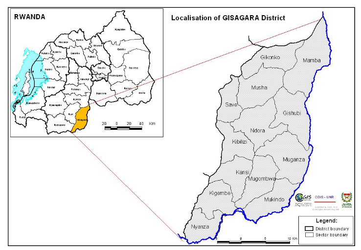
Appendix 3 : Gisagara District's administrative map
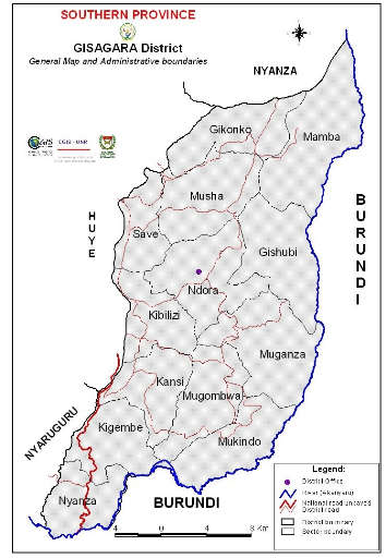
| 

