|
KIGALI INSTITUTE OF SCIENCE AND TECHNOLOGY
(KIST)
INSTITUT DES SCIENCES ET TECHNOLOGIE DE
KIGALI
Avenue de l'armée, BP 3900 KIGALI-RWANDA

FACULTY OF ENGINEERING
DEPARTEMENT OF ELECTRICAL AND ELECTRONICS
ENGINEERING
CERTIFICATE
This is to certify that the project work entitled»
Implementation of edge detection for digital image» is a
record of original property work done by:
HARELIMANA Joyeuse (GS20031000),
MBARUBUKEYE Innocent (GS20031281),
NYIRANGENDAHIMANA Stephanie (GS20031373),
in the partial fulfillment of the requirement for the award of
Bachelor of Science in Electrical and Electronics Engineering Department (EEE)
of Kigali Institute of Science and Technology during the academic year 2007.
This dissertation fulfills the requirement of the institute
regulations relating to the nature and standards of works for the award of
Bachelor of Science in Electronics and Telecommunication Engineering Degree.
Date......../......../........
.................... ..... .....
.................................
Mr. RUBESH Anand
Dr.Eng. NTAGWIRUMUGARA
Etienne.
Supervisor
Head of Department
DECLARATION
We, HARELIMANA Joyeuse (GS20031000), MBARUBUKEYE Innocent
(GS20031281), NYIRANGENDAHIMANA Stéphanie (GS20031373), declare that all
the work presented in this report is original.
To the best of our knowledge, the same work has never
presented in KIST or any other universities or institutions of high
learning.
A reference though was done and was provided from other
people's work therefore, we declare that this work is ours.
Signed by:
Joyeuse HARELIMANA
.....................................
Innocent MBARUBUKEYE
..................................
Stephanie NYIRANGENDAHIMANA
.......................................
DEDICATION.
To our God and our savior Jesus,
To our beloved parents,
To our brothers and sisters,
To our families and
To all our close friends
We dedicate this work.
ACKNOWLEDGEMENT
First we would like to thank the Almighty GOD for keeping us
alive during our whole study.
We express our gratitude to every one who contributes in our
studies, especially to our government, who gives us the opportunity of studding
at high learning institution and KIST administration board who gave us
financial support for this final year project.
We would like to thank all staffs of Electrical and
Electronics Engineering Department in KIST and Estates Officer for their
support and extra knowledge, which they gave us.
We would like to extend special thanks to our supervisor Mr.
RUBESH Anand for giving up many ideas and essential hint to support my research
to be conducted.
We express our deep gratitude to Mr. Kanyarubira J.Baptiste,
Mr. Nsekanabo Emmanuel and Mr. Nyirimihigo Célestin for their greater
support without them we will not finish this work.
We are especially grateful to our parents whose patience;
encouragement and understanding were vital to the completion of this study.
Once again it is pleasure to acknowledge all people who
support us directly and indirectly in completion of this project.
We wish them all the best.
ABSTRACT
The world is growing up in information technology where the
processing of images is required also. From the past until now, human being is
seeking how to improve knowledge and updating system from oldest to the latest
ones.
As memorial, in past, human used scripts and drawing for keeping
images to be used in future but that oldest technology was so poor because it
took along time to achieve it.
After that, analog pictures and image processing came on,
whereby analog cameras were used. This was so fast and doest not require energy
and forces for processing it.
But the worst of this analog technology is the storage of this
image and no further processing which can be carried out on this. As solution,
the digital image processing is widely used for overcoming a problem of storing
and further processing that has been observed in analog image processing.
In digital image processing, different technologies along with
computer are used for better image processing. This work of digital image
processing, the focus is on Edge detection for digital
images.
In the oldest research, the different technologies such as
photometric and geometric models are used whereby some failures were
experienced.
During our work, these failures and difficulties are overcoming
by using MATLAB software where the edges of image are well and easier detected.
LIST OF FIGURES AND
TABLES.
Figure 2.1: Fundamental steps in digital image
processing..........................................6
Table 2..4.1: shows the two Roberts Cross
kernels....................................................18
Table 2..4.2: shows the sobel
kernel...........................................................................20
Table 2..4.3: shows Prewitt's
mask............................................................................22
Table 3.1.a: shows product and comand
used............................................................35
Table 3.1.b: shows Excel files to use with each Excel
version..................................35
Table 3.1.c: shows finding information about
matlab...............................................35
Table 3.1.d: shows conversion between different
formats........................................47
Table 3.1: conversion between image
types.............................................................48
Table 4.1: shws comparison of number of pixels between PNG, GIF,
BMP file formats and JPEG file
format.....................................................................................62
Table 4.2: shows the results based on variation of contrast
and brightness...............64
NOMENCLATURE
LIST.
BMP: Bitmap file format
CCD: charge couple device
e.g.: example given
eq.: equation
Fig.: figure
HDF: Hierarchical Data Format
I/O: Input/Output
IEEE: Institute of Electrical and
Electronics Engineers
JPEG: Joint Photography Experts Group
KIST: Kigali Institute of Science and
Technology
LCD: Liquid Crystal Display
LUT: Look Up Table
RGB: Red Green and Blue
SI: System International
SLR: Single Lens Reflex
TIFF: Tagged Image File Format
VDT: Video Display Terminal
i.e.: id est
LZW: Lempel-Ziv-Welch
DSC: Digital Still Cameras
CMOS: Complementary Metal Oxide
Semiconductors
DC: Direct Current
DSLRs: Digital Single-Lens Reflex cameras
PNG: Portable Network Graphics
GIF: Graphic Interchange Format
TABLE OF
CONTENTS
CERTIFICATE
i
DECLARATION
ii
DEDICATION.
iii
ACKNOWLEDGEMENT
iv
ABSTRACT
v
LIST OF FIGURES AND TABLES.
vi
NOMENCLATURE LIST.
vii
TABLE OF CONTENTS
viii
CHAPTER 1. INTRODUCTION
1
1.1. GENERAL INTRODUCTION.
1
1.2 PROBLEM IDENTIFICATION.
2
1.3. SCOPE OF THE STUDY.
2
1.4. TECHNIQUES USED.
2
1.5. OBJECTIVES OF THE PROJECT.
2
1.6. PROJECT OUTLINE.
2
CHAPTER 2. LITERATURE REVIEW.
4
2.1 INTRODUCTION TO THE IMAGE.
4
2.1.0. Digital image.
4
2.1.1. Digital image processing
4
2.1.2. Fundamental steps in digital image
processing
6
2.1.3. Image segmentation
8
2.1.4. Image representation
8
2.2 DIGITAL COMPUTER
9
2.2.1. Definition of digital computer
9
2.2.2. Working of computers.
9
2.3. INTRODUCTION TO CAMERAS.
9
2.3.0. Film cameras
9
2.3.1. Digital cameras
10
2.4. EDGE DETECTION
14
2.4.1 Introduction to the edge detection
14
2.4.2 Edge properties.
16
2.4.3 Detecting an edge.
16
2.4.4 Edge detection algorithms.
17
2.5. PIXELS
22
2.6. PRIMARY COLOURS
25
2.7. MULTI-SPECTRAL IMAGES
26
2.8. LOOK UP TABLES AND COLOURMAPS
27
2.9. LUMINOUS INTENSITY
28
2.10. GAUSSIAN SMOOTHING
30
2.11. FACE IDENTIFICATION.
31
CHAPTER 3. RESEARCH METHODOLOGY.
32
3.1. METHOD USED AND SOFTWARE DEVELOPMENT.
32
3.1.1. Definition of matlab.
32
3.1.3. Function used by matlab.
35
3.1.4. Commands used.
38
3.1.5. Symboles used.
38
3.1.6. To write matlab programs
39
3.1.7. To end a program.
41
3.1.8. Access to implementation details
41
3.1.9. Fundamentals on matlab.
42
3.1.10. Image types and data classes
43
3.1.11. Conversion between different formats
46
3.2. EQUIPMENTS USED.
47
3.3. MATERIALS USED.
47
3.4. DETECTING AN OBJECT USING IMAGE
SEGMENTATION.
47
3.5. IMPLEMENTATION OF EDGE DETECTION.
50
CHAPTER 4. RESULTS AND DISCUSSION.
60
4.1. RESULTS.
60
4.2. DISCUSSION.
63
CHAPTER 5. CONCLUSION AND
RECOMMENDATION.
64
5.1. CONCLUSION.
64
5.2. RECOMMENDATION.
64
REFERENCES.
65
APPENDICES
66
CHAPTER 1.
INTRODUCTION
1.1. GENERAL
INTRODUCTION.
Edge detection in the human brain takes place automatically.
It is an important concept both in the area of image processing and in the area
of object recognition, Without being able to determine where the edge of an
object fall, a machine would be able unable to determine many things about that
object such as shape, volume, and area. Being able to recognize an object is a
key step towards the development of artificial intelligence.
Edge detection is the process of localizing pixel intensity
transitions. The edge detection have been used by object recognition, target
tracking, segmentation, and etc. Therefore, the edge detection is one of the
most important parts of image processing.
Edge detection can be used for numerous applications in which
access to an article is to be restricted to a limited number of persons.
The edge detection offers several benefits including simplicity,
convenience, security and accuracy.
The edge detection is an important in most image processing
techniques. It can identify the area of image where large change in intensity
occurs.
These changes are associated with the physical boundary or
edge in the scene from which the image is derived.
There are many techniques used in edge detection, but most of
them can be grouped into two categories:
1. Search based and
2. Zero crossing based.
The search-based methods detect edges by looking for maxima
and minima in the first derivative of an image.
The zero crossing based methods: search for zero crossing in the
2nd derivative of the image in the order to find an image.
The area where images are processed using proprietary
software, for example Photoshop where the implementation details of any image
processing algorithm are inaccessible. Some algorithms are quite complex and
the result may be sensible to subtleties in the implementation. An image that
has been extensively processed using proprietary software may well be
challenged in court. This problem is solved by using MATLAB software which may
not be as user friendly as an application like Photoshop; however, being a
general purpose programming language it provides many important advantages for
forensic image processing.
1.2 PROBLEM
IDENTIFICATION.
As already started in the introduction, edge detection is used to
detect an object (solid object). Not only the image detection, but also the
intensity of gray-level of that object is noted.
There are some software used to process image and the
implementation details of any image processing algorithm are inaccessible (lack
of using programming language). Our project is focused on software used to
detect edges of image employing mainly the MATLAB program for solving this
problem.
1.3. SCOPE OF THE STUDY.
The areas of this work are in electronics and telecommunication
engineering, which are very wide fields.
This work is intended to implement the edge detection for
digital image, so that it may be carried out to a big contour (face)
identification of an object (an image).
1.4. TECHNIQUES USED.
In order to accomplish this task, the researchers require the use
of the following methods:
· The study guide utilizes an extensive conversation
containing edge detection objectives.
· Library search was used to find background of digital
image processing in this project.
· Websites consultancies.
General methods and techniques were used to collect for this
project as primary as well as secondary data collection. Secondary data was
collected from published materials related to the topic. These include: book
class notes and online information by visiting some websites on the
Internet.
1.5. OBJECTIVES OF THE
PROJECT.
The objectives of this project are the following:
1. To face identification of an object.
2. To implement an edge detection for digital image.
1.6. PROJECT OUTLINE.
The outline of this project consists of five chapters.
The first is Introduction. It discusses the
motivation for the work is being reported, provides a brief overview of each of
the main chapters that the reader will encounter.
The second chapter is Literature review, which
provides details about what other others have done and hence set a benchmark
for the current project as well as to justify the use of specific solution
techniques.
The third chapter is Research methodology. This
chapter deals with the methodology and materials used.
The fourth chapter is Results and discussion. It
deals with the analysis of results obtained from different file format of
images used in this work.
This section presents the results from experiments or survey.
The fifth chapter is conclusion and
recommendation. It gives summary of the main findings also the problems
limitation is discussed.
.
CHAPTER 2. LITERATURE
REVIEW.
2.1 INTRODUCTION TO THE
IMAGE.
2.1.0. DIGITAL IMAGE.
An image may be defined as a two-dimensional function, f (x,y),
where x and y are special(plane) coordinates, and the amplitude of f at any
pair of coordinates (x,y) is called intensity or grey- level of the image at
that point.
When x, y and the amplitude values of f are all finite, discrete
quantities, we call this image a digital image.
2.1.1. DIGITAL IMAGE
PROCESSING
Image processing: is to perform a particular series of operation
on that image, such a set of the field of digital image processing refers to
processing digital images by means of a digital computer.
Note that a digital image is composed of a finite number of
elements, each of which has a particular location and value.
These elements are referred to as picture elements, images
elements, pels and pixels.
The area of an image analysis (also called image understanding)
is in between image processing and computer vision.
There are no clear-cut boundaries in the continuum from image
processing at one end to computer vision at the other. However one useful
paradigm is to consider three types of computerized processes in this
continuum: low-level, mid-level and high level processes.
Low-level process: involves primitive operation
such as image processing to reduce noise, contrast enhancement and image
sharpening. A low level process is characterised by the fact that both its
inputs and outputs are images.
Mid-level processing on images: involves task
such as segmentation (partitioning an image into regions or objects),
description of those objects to reduce them to a form suitable for computer
processing and classification (recognition) of individual objects.
A mid-level process is characterized by the fact that its input
general is images, but its outputs are attributes extracted from those images.
(Example: edges, contours, and the identity of individual objects).
Finally, high level processing involves making sense, of an
ensemble of recognized objects, as in image analysis, and, at the far end of
the continuum, performing the cognitive function normally associated with
vision.
Based on the preceding comments, we see that a logical place of
overlap between image processing and image analysis is the area of recognition
of individual regions or objects in an image.
Thus, what we call in this book digital image processing
encompasses processes whose inputs and outputs are images and, in addition
encompasses processes that extract attributes from images, up to and including
the recognition of individual object.
Digital Image Processing (DIP) is a
multidisciplinary science that borrows principles from diverse fields such as
optic, surface physique, visuals psychophysics, computer science, and
mathematics. The main application of image processing include: astronomy,
ultrasonic imaging, remote sensing, Video communication and microscopy, among
innumerable others.
In digital image processing system, an image processor reads out
image data from a window of an image buffer memory having N-columns and M-
rows.
2.1.2. FUNDAMENTAL STEPS IN
DIGITAL IMAGE PROCESSING
Image Acquisition
Knowledge Base
Object Recognition
Representation &Description
Segmentation
Morphological processing
Compression
Wavelets and
Multi-resolution processing
Color image
Processing
Image Restoration
Image Enhancement


Figure 2.1: Fundamental steps in digital image
processing.[3]
It is helpful to divide the material covered in image
processing into the two broad
categories methods whose inputs and outputs are images, and
methods whose inputs may be images, but whose outputs are attributing extracted
from those images. This organization is summarized in fig.2.1 above.
The diagram does not imply that every process an applied to an
image, but the intension is to convey an idea of all the methodologies that can
be applied to images for different purposes and possibly with different
objectives.
The discussion of this section is as follow:
1. Image acquisition: note that acquisition
could be as simple as being given an image that is already in digital form.
Generally, image acquisition stage involves pre-processing such as scaling.
2. Image enhancement: is among the simplest
and most appealing areas of digital image processing. Basically, the idea
behind enhancement techniques is to bring out detail that is obscured, or
simply to highlight certain features of interest in an image. A familiar
example of enhancement is when we increase the contrast of an image because
«it looks better».
3. Image restoration: is an area that also
deals with improving the appearance of an image. However, unlike enhancement,
which is subjective, image restoration is objective, in the sense that
restoration techniques tend to be based on mathematical or probabilistic models
of image degradation. Enhancement, on the other hand, is based on human
subjective preferences regarding what constitutes a «good»
enhancement result.
4. Colour image processing: is an area that
has been gaining in importance because of the significant increase in the use
of digital images over the Internet.
5. Wavelets: are the foundations for
representing images in various degrees of resolution (approving). In
particular, this material is used for image data compression and for pyramidal
representation, in which images are subdivided successively into smaller
regions.
6. Compression: as the name implies, deals
with techniques for reducing the storage required saving an image, or the
bandwidth required transmitting it. Image compression is familiar (perhaps in
advertently) to most users of computers in the form of image file extension,
such as the jpg file extension used in JPEG image compression standard.
7. Morphological processing: deals with tools
for extracting image components that are useful in the representation and
description of shape. The material in this processing begins a transition from
processes that output images to processes that output image attributes.
8. Representation and description: almost
always follow the output of a segmentation stage, which usually is raw pixels
data, constituting either the boundary of a region (i.e. the set of pixels
separating one image region from another) or all the points in the region
itself. In either case, converting the data to a form suitable for computer
processing is necessary. The first decision that must be made is whether the
data should be represented as a boundary or as s complete region.
Boundary representation is appropriate when the focus is on
external shape characteristics, such as corners, and inflection. Choosing a
representation is only part of the solution for transforming raw data into a
form suitable for subsequent computer processing.
Description, also called feature selection, deals with
extracting attributes that result in some quantitative information of interest
or are basic for differentiating one class of objects from another.
9. Recognition: is the process that assigns a
label to an object based on its description. So far we have said nothing about
the need for prior knowledge or about the interaction between the knowledge
base and the processing modules in fig.2.1.
Knowledge about a problem domain is coded into an image
processing system in the form of a knowledge database. This
knowledge may be as simple as detailing regions of images where the information
of interest is known to be located, thus limiting the search that has to be
conducted in seeking that information. The knowledge base also can be quite
complex, such as an interrelated list of all major possible defects in a
materials inspection problem or an image database containing high-resolution
satellite images of a region in connection with change-detection
applications.
In addition to guiding the operation of each processing
module, the knowledge base also controls the interaction between modules.
This distinction is made in fig.2.1 by the use of
double-headed arrows between the processing modules and the knowledge base, as
opposed to single-headed arrows linking the processing modules.
2.1.3. IMAGE
SEGMENTATION
Image segmentation is the material in the previous section
2.1.2 began a transition from an image processing methods whose input and
output are images, to methods in which the input are images, but the outputs
are attributes extracted from those images. Segmentation is another major step
in that direction.
Image segmentation algorithms general are based on two basic
properties of intensity values: discontinuities and similarity. In the first
category, the approach is to partition an image based on abrupt changes in
intensity, such as edges in an image.
The principle approach in second category is based on
partitioning an image into regions that are similar according to a set of
predefined criteria.
Thresholding, region growing, and region splitting and merging
are examples of methods in this category.
2.1.4. IMAGE
REPRESENTATION
An image is stored as a matrix using standard Matlab matrix
conventions. There are five basic types of images supported by Matlab:
Indexed images
Intensity images
Binary images
RGB images
8-bit images
2.2 DIGITAL COMPUTER
2.2.1. DEFINITION OF
DIGITAL COMPUTER
A digital computer is a combination of digital devices and
circuits that can perform a programmed sequence of operations with a minimum of
human intervention.
The sequence of operations is called a program.
The program is a set of coded instruction that is stored in
the computer's internal memory along with all of the data that the program
requires.
When the computer is commanded to execute the program, it
performs the instructions in the order that they are stored in memory until the
program is completed.
It does his at extremely high speed
2.2.2. WORKING OF
COMPUTERS.
Computers do not think, the computer programmer provides a
program of instruction and data that specifies very detail of what to do, what
to do it to, and when to do it.
The computer is simply a high-speed machine that can
manipulate data, solve problems, and make decision, all under the control of
the program.
If a programmer makes a mistake in the program or puts in the
wrong data, the computer will produce wrong results. A popular saying in the
computer field is garbage in/garbage out.
2.3. INTRODUCTION TO
CAMERAS.
2.3.0. FILM CAMERAS
Film cameras are the cameras whose use films in recording images
as photographs or as a moving picture.
ELEMENTS OF FILM CAMERAS
A still film camera is made of three basic elements: an optical
element (the lens), a chemical element (the film) and a mechanical element (the
camera body itself). As we'll see, the only trick to photography is calibrating
and combining these elements in such a way that they record a crisp,
recognizable image.
There are many different ways of bringing everything together. In
this article, we'll look at a manual single-lens-reflex (SLR)
camera. This is a camera where the photographer sees exactly the same image
that is exposed to the film and can adjust everything by turning dials and
clicking buttons. Since it doesn't need any electricity to take a picture, a
manual SLR camera provides an excellent illustration of the fundamental
processes of photography.
The optical component of the camera is the lens.
At its simplest, a lens is just a curved piece of glass or plastic. Its job is
to take the beams of light bouncing off of an object and redirect them so they
come together to form a real image an image that looks just
like the scene in front of the lens.
2.3.1. DIGITAL CAMERAS
2.3.1.0. DEFINITION OF DIGITAL CAMERA.
A digital camera is an
electronic device used
to capture and store
photographs digitally,
instead of using
photographic film
like conventional
cameras, or recording images
in an analog format to
magnetic tape like
many
video cameras. Modern
compact digital cameras are typically multifunctional, with some devices
capable of recording
sound and/or
video as well as
photographs.
2.3.1.1. CLASSIFICATION OF DIGITAL CAMERAS
Digital cameras can be classified into several categories:
· Video cameras
· live preview digital cameras
· Digital single lens reflex cameras
· Digital range finders
· Professional modular digital cameras systems
· Line scan cameras system
VIDEO CAMERAS
Video cameras are classified as devices whose main purpose is to
record moving images.
Professional
video cameras such as those used in
television and
movie production. These
typically have multiple image sensors (one per color) to enhance
resolution and
color gamut.
Professional video cameras usually do not have a built-in
VCR or
microphone
They generally include a microphone to record sound, and feature
a small
liquid crystal
display to watch the video during taping and playback.
LIVE PREVIEW DIGITAL CAMERAS
In addition, many
Live-Preview
Digital cameras have a "movie" mode, in which images are continuously
acquired at a frame rate sufficient for video.
Main article:
Live-preview
digital camera
The term digital still camera (DSC) most commonly refers
to the class of live-preview digital cameras, cameras that use an
electronic screen as the principal means of framing and previewing before
taking the photograph. All use either a
charge-coupled
device (CCD) or a
CMOS
image sensor to sense
the light intensities across the focal plane.
Many modern live-preview cameras have a movie mode, and a growing
number of
camcorders can take still
photographs.
DIGITAL SINGLE LENS REFLEX CAMERAS
Digital single-lens reflex cameras (DSLRs) are digital cameras
based on film
single-lens
reflex cameras (SLRs), both types are characterized by the existence of a
mirror and reflex system. See the main article on
DSLRs
for a detailed treatment of this category.
DIGITAL RANGE FINDERS
A rangefinder is a focusing mechanism once widely used on film
cameras, but much less common in digital cameras. The term rangefinder
alone is often used to mean a rangefinder camera, that is, a camera equipped
with a rangefinder
PROFESSIONAL MODOLAR DIGITAL CAMERA SYSTEMS
This category includes very high end professional equipment
that can be assembled from modular components (winders, grips, lenses, etc.) to
suit particular purposes. Common makes include Hasselblad and Mamiya. They were
developed for medium or large format film sizes, as these captured greater
detail and could be enlarged more than 35mm.
Typically these cameras are used in studios for commercial
production
LINE SCAN CAMERAS SYSTEM
A line-scan camera is a camera device containing a line-scan
image sensor chip, and
a focusing mechanism. These cameras are almost solely used in industrial
settings to capture an image of a constant stream of moving material. Unlike
video cameras, line-scan cameras use a single array of
pixel sensors,
instead of a matrix of them. Data coming from the line-scan camera has a
frequency, where the camera scans a line, waits, and repeats. The data coming
from the line-scan camera is commonly processed by a computer, to collect the
one-dimensional line data and to create a two-dimensional image. The collected
two-dimensional image data is then processed by image-processing methods for
industrial purposes.
2.3.1.2. IMAGE RESOLUTION
The
resolution of a
digital camera is often limited by the camera
sensor (usually a
charge-coupled device or
CCD chip) that
turns light into discrete signals, replacing the job of film in traditional
photography. The sensor is made up of millions of "buckets" that collect charge
in response to light. Generally, these buckets respond to only a narrow range
of light wavelengths, due to a color
filter over
each. Each one of these buckets is called a
pixel, and a
demosaicing/interpolation
algorithm is needed to turn the image with only one wavelength range per pixel
into an
RGB image where each pixel is
three numbers to represent a complete color.
The one attribute most commonly compared on cameras is the
pixel count. Due to the ever increasing sizes of sensors, the pixel count is
into the millions, and using the
SI prefix of
mega- (which means 1 million) the pixel counts are given in
megapixels. For example, an 8.0 megapixel camera has 8.0 million pixels.
The pixel count alone is commonly presumed to indicate the
resolution of a camera, but this is a misconception. There are several other
factors that impact a sensor's resolution. Some of these factors include sensor
size, lens quality, and the organization of the pixels (for example, a
monochrome camera without a
Bayer filter mosaic has
a higher resolution than a typical color camera). Many digital compact cameras
are criticized for having excessive pixels, in that the sensors can be so small
that the resolution of the sensor is greater than the lens could possibly
deliver.
2.3.1.3. METHODS OF IMAGES CAPTURE
This digital camera is partly disassembled. The lens assembly
(bottom right) is removed, but the sensor (top right) still captures a usable
image, as seen on the LCD screen (bottom left).
Since the first digital backs were introduced, there have been
three main methods of capturing the image, each based on the hardware
configuration of the sensor and color filters.
The first method is often called single-shot, in
reference to the number of times the camera's sensor is exposed to the light
passing through the camera lens. Single-shot capture systems use either one CCD
with a
Bayer filter mosaic it,
or three separate
image sensors (one each
for the
primary additive
colors red, green, and blue) which are exposed to the same image via a beam
splitter.
The second method is referred to as multi-shot
because the sensor is exposed to the image in a sequence of three or more
openings of the lens aperture. There are several methods of application of the
multi-shot technique. The most common originally was to use a single
image sensor with three
filters (once again red, green and blue) passed in front of the sensor in
sequence to obtain the additive color information. Another multiple shot method
utilized a single CCD with a Bayer filter but actually moved the physical
location of the sensor chip on the focus plane of the lens to "stitch" together
a higher resolution image than the CCD would allow otherwise. A third version
combined the two methods without a Bayer filter on the chip.
The third method is called scanning because the
sensor moves across the focal plane much like the sensor of a desktop scanner.
Their linear or tri-linear sensors utilize only a single line
of photosensors, or three lines for the three colors. In some cases, scanning
is accomplished by rotating the whole camera; a digital
rotating line
camera offers images of very high total resolution.
The choice of method for a given capture is of course
determined largely by the subject matter. It is usually inappropriate to
attempt to capture a subject that moves with anything but a single-shot system.
However, the higher color fidelity and larger file sizes and resolutions
available with multi-shot and scanning backs make them attractive for
commercial photographers working with stationary subjects and large-format
photographs. CMOS-based single shot cameras are also somewhat common.[5]
2.3.1.4. IMAGE FILE FORMATS.
Common formats for digital camera images are the Joint
Photography Experts Group standard (
JPEG) and Tagged Image File
Format (
TIFF).
They usually store images in one of two formats TIFF, which is
uncompressed, and JPEG, which is compressed. Most cameras use the JPEG file
format for storing pictures, and they sometimes offer quality settings (such as
medium or high).
JPEG is a compression algorithm developed by people the format
is named after, the Joint Photographic Experts Group.
JPEG is big selling point is that its compression factor
stores the image on the hard drive in less bytes than the image is when it
actually displays.
JPEG uses lossy compression (lossy meaning "with losses to
quality"). Lossy means that some image quality is lost when the JPG data is
compressed and saved, and this quality can never be recovered.
TIFF - Tag Image File Format
TIFF is the format of choice for archiving important images.
TIFF is THE leading commercial and professional image standard. TIFF is the
most universal and most widely supported format across all platforms, Mac,
Windows, Unix. Data up to 48 bits is supported.
TIFF image files optionally use LZW lossless compression.
Lossless means there is no quality loss due to compression. Lossless guarantees
that you can always read back exactly what you thought you saved, bit-for-bit
identical, without data corruption. This is a critical factor for archiving
master copies of important images. Most image compression formats are lossless,
with JPG and PCD files being the main exceptions
Graphic Interchange Format (GIF)
GIF was developed by CompuServe to show images online (in 1987
for 8 bit video boards, before JPG and 24 bit color was in use). GIF uses
indexed color, which is limited to a palette of only 256 colors (next page).
GIF was a great match for the old 8 bit 256 color video boards, but is
inappropriate for today's 24 bit photo images.
PNG - Portable Network Graphics
PNG is not so popular yet, but it's appeal is growing as
people discover what it can do. PNG was designed recently, with the experience
advantage of knowing all that went before. The original purpose of PNG was to
be a royalty-free GIF and LZW replacement. However PNG supports a large set of
technical features. Compression in PNG is called the ZIP method.
2.3.1.5 IMAGE CAPTURING
A light source say a candle emits light in all directions. The
rays of light all start at the same point the candle's flame and then are
constantly diverging. A converging lens takes those rays and redirects them so
they are all converging back to one point. At the point where the rays
converge, you get a real image of the candle.
2.3.1.6 DIFFERENCE BETWEEN FILM CAMERAS AND DIGITAL
CAMERAS
The digital camera is one of the most remarkable instances of
this shift because it is so truly different from its predecessor. Conventional
cameras depend entirely on chemical and mechanical processes you don't even
need electricity to operate them. On the other hand, all digital cameras have a
built-in computer, and all of them record images electronically.
The new approach has been enormously successful. Since film
still provides better picture quality, digital cameras have not completely
replaced conventional cameras. But, as digital imaging technology has improved,
digital cameras have rapidly become more popular.
2.4. EDGE DETECTION
2.4.1 INTRODUCTION TO THE
EDGE DETECTION
Edge detection is the process of localizing pixel intensity
transitions. The edge detection
have been used by object recognition, target tracking,
segmentation, and etc. Therefore, the edge detection is one of the most
important parts of image processing.
There mainly exist several edge detection methods (Sobel,
Prewitt, Roberts, Canny ). These methods have been proposed for detecting
transitions in images. Early methods determined the best gradient operator to
detect sharp intensity variations .
Commonly used method for detecting edges is to apply
derivative operators on images.
Derivative based approaches can be categorized into two
groups, namely first and second order derivative methods. First order
derivative based techniques depend on computing the gradient several directions
and combining the result of each gradient. The value of the gradient magnitude
and orientation is estimated using two differentiation masks. In this work,
Sobel which is an edge detection method is considered. Because of the
simplicity and common uses, this method is preferred by the others methods in
this work. The Sobel edge detector uses two masks, one vertical and one
horizontal. These masks are generally used 3×3 matrices. Especially, the
matrices which have 3×3 dimensions are used in matlab. The masks of the
Sobel edge detection are extended to 5×5 dimensions, are constructed in
this work. A matlab function, called as Sobel 5×5, is developed by using
these new matrices. Matlab, which is a product of The Mathworks Company,
contains has a lot of toolboxes. One of these toolboxes is image toolbox which
has many functions and algorithms. Edge function which contains several
detection methods (Sobel, Prewitt,Roberts, Canny, etc) is used by the user.
The image set, which consist of 8 images (256×256), is
used to test Sobel 3×3 and
Sobel 5×5 edge detectors in matlab.
Edge detection is one of the techniques used for detecting the
gray-level discontinuities.
It is the most common approach for detecting meaningful
discontinuities in gray-level.[3]
Edge detection is an important concept, both in the area of
image processing and in the area of object recognition. Without being able to
determine where the edges of an object fall a machine would be unable to
determine many things about that object such as shape, volume, area and so
forth. Being able to recognize an object is a key step towards the development
of artificial intelligence.
The goal of edge detection is to mark the points in a digital
image at which the luminous intensity changes sharply. Edge detection of an
image reduces significantly the amount of data and filters out information that
may be regarded as less relevant, preserving the important structural
properties of an image.
2.4.2 EDGE PROPERTIES.
Edges may be viewpoint dependent - these are edges that may
change as the viewpoint changes, and typically reflect the geometry of the
scene, objects occluding one another and so on, or may be viewpoint independent
- these generally reflect properties of the viewed objects such as surface
markings and surface shape.
Edges play quite an important role in many applications of image
processing.
Edge detection of an image reduces significantly the amount of
data and filters out information that may be regarded as less relevant,
preserving the important structural properties of an image. There are many
techniques for edge detection, but most of them can be grouped into two
categories: Search-based and zero-crossing based.
-The search-based methods detect edges by looking for maxima
and minima in the first derivative of the image, usually local directional
maxima of the gradient magnitude.
-The zero-crossing based methods search for zero crossings in
the second derivative of the image in order to find edges.
2.4.3 DETECTING AN
EDGE.
Taking an edge to be a change in intensity taking place over a
number of pixels, edge detection algorithms generally compute a derivative of
this intensity change.
COMPUTING THE 1st DERIVATIVE
Many edge-detection operators are based upon the
1st derivative of the intensity - this gives us the intensity
gradient of the original data. Using this information we can search an image
for peaks in the intensity gradient.
For higher performance image processing, the 1st derivative
can therefore be calculated (in 1D) by convolving the original data with a
mask:
The magnitude of the first derivative can be used to detect
the presence of an edge at a point in an image.
COMPUTING THE 2nd DERIVATIVE
Some other edge-detection operators are based upon the 2nd
derivative of the intensity. This is essentially the rate of change in
intensity gradient.
Here, we can alternatively search for zero-crossings in the
second derivative of the image gradient.
Again most algorithms use a convolution mask to quickly process
the image data:
The signs of the 2nd derivative can be used to
determine whether an edge pixel lies on the dark or light side of an
edge.[17]
THRESHOLDING
Once we have calculated our derivative, the next stage is to
apply a threshold, to determine where the result suggests an edge to be
present. It is useful to be able to separate out the regions of the image
corresponding to the objects in which we are interested, from the region of the
image that correspond to background. Threshold often provides n easy and
convenient way to perform this segmentation.
Thresholding is the simplest method of image segmentation on
the basis of deferent intensities in the foreground and background regions of
an image. Individual pixels in image are marked as «object» if their
value is greater than some threshold value.(assuming an object to be bright
than the background) and as» background «pixels if their values is
less than threshold value. The key parameter in thresholding is the choice of a
threshold.
Several different methods for choosing a threshold exist. But
a common used compromiser method is thresholding with hysteresis. This method
uses multiple thresholds to find edges. We begin by using the upper threshold
to fid the start point. Once we have a start point, we trace the edge's path
through the image pixel by pixel, marking an edge whenever we are above the
lower threshold. We stop marking our edge only when the value falls below our
low threshold.
2.4.4 EDGE DETECTION
ALGORITHMS.
An edge, by definition, is that drastic change in value from
one spot to the next either in an image or in one's own eyes. In the digital
world, an edge is a set of connected pixels that lie on the boundary between
two regions. Ideally, a digital edge would have one pixel colored a certain
value and one of its neighboring pixels colored noticeably different. Since the
contrast between the pixels is drastic, we label it an edge. Unfortunately,
when dealing with digital pictures, most edges are blurred. This leads to edges
having a gradual change of pixels levels from one object to the next thus
causing the edge to be less defined and harder to distinguish. In this
instance, one would have to devise an intuitive way to distinguish gray level
transitions.
Edge detection is the process of determining where the
boundaries of objects fall within an image. There are several algorithms that
exist to date that are able detect edges. Roberts Cross was the first technique
used and is thus the fasted and simplest to implement. Lastly, there is the
Canny edge detection algorithm. This uses several steps to detect edges in an
image. However, this algorithm can be slow at times due to its higher degree of
complexity.
1. ROBERTS CROSS EDGE DETECTION
The Roberts Cross algorithm performs a two dimensional spatial
gradient convolution on the image. The main idea is to bring out the horizontal
and vertical edges individually and then to put them together for the resulting
edge detection.
|
We have two typical Roberts Cross kernels .
|
|
+100-1
|
0+1-10
|
Table 2.4.1: shows the two Roberts Cross
kernels.
The two Roberts Cross kernels, shown above in Figure 1, are
designed with the intention of bringing out the diagonal edges within the
image. The Gx image will enunciate diagonals that run from the top-left to the
bottom-right where as the Gy image will bring out edges that run top-right to
bottom-left. The two individual images Gx and Gy are combined using the
approximation equation
|G| = |Gx| + |Gy|.
Roberts Cross is not quite as effective as the Sobel
technique. It does bring out edges, but when compared the same image only using
the Sobel algorithm, the amount of edges detected is poor. The Sobel approach
seems to work the best.
In general, kernels are designed so that it consists of an odd
number of rows and columns. This helps to define a distinct center in each
kernel. Sampling pixels on each side of the center pixel leads to a better
convolution image. This yields a better edge detection image produced in the
outcome. The Sobel algorithm takes this account into effect when selecting its
kernels.
2. SOBEL EDGE DETECTION
Overview of sobel edge detection.
Standard Sobel operators, for a 3×3 neighborhood, each
simple central gradient
estimate is vector sum of a pair of orthogonal vectors . Each
orthogonal vector is a directional derivative estimate multiplied by a unit
vector specifying the derivative's direction. The vector sum of these simple
gradient estimates amounts to a vector sum of the 8 directional derivative
vectors.
Sobel which is a popular edge detection method is considered
in this work. There exists a function, edge.m which is in the image toolbox. In
the edge function, the Sobel method uses the derivative approximation to find
edges. Therefore, it returns edges at those points where the gradient of the
considered image is maximum. The horizontal and vertical gradient matrices
whose dimensions are 3×3 for the Sobel method has been generally used in
the edge detection operations. In this work, a function is developed to find
edges using the matrices whose dimensions are 5×5 in matlab.
Edge detection function
Each direction of Sobel masks is applied to an image, and then
two new images are created. One image shows the vertical response and the other
shows the horizontal response. Two images combined into a single image. The
purpose is to determine the existence and location of edges in a picture. This
two image combination is explained that the square of created masks pixel
estimate coincidence each other as coordinate are summed. Thus new image on
which edge pixels are located obtained the value which is the squared of the
above summation. The value of threshold in this above process is used to detect
edge pixels.
An algorithm is developed to find edges using the new matrices
and then, a matlab function, which is called as Sobel 5x5.m, is implemented in
matlab. This matlab function requires a grayscale intensity image,
two-dimensional array. The result which is returned by this function is the
final image in which the edge pixels are denoted by white color.
|
The sobel Edge detection algorithm uses the following two
kernels.
|
|
+1+2+1000-1-2-1
|
-10+1-20+2-10+1
|
Table 2.4.2: shows the sobel kernels.
The Sobel kernels, as shown in the above figure, are larger
than its predecessor, the Roberts Cross, is. This causes the processes to be
less susceptible to noise.
As one can see, there are only really two pixels of concern
with the Roberts Cross algorithm thus noise can be a rather large issue. The
Sobel algorithm deals with six pixels and in doing so takes a better average of
the neighboring pixels. This along with slight blurring can eliminate most
noise found within normal images.
3. CANNY EDGE DETECTION
This is another method of detecting edge.
First the image is run through a Gaussian blur to help get
ride of a majority of the noise. Second, an edge detection algorithm is applied
such as the Roberts Cross or Sobel techniques. From there the angle and
magnitude can be obtained and used to determine which portions of the edges
should be suppressed and which should be brought out. Lastly, there are two
threshold cutoff points. Any value in the image below the first threshold is
dropped to zero. Any value above the second threshold is raised to one. For any
pixels whose values fall within the two thresholds, their values are set to
zero or one, based on their neighboring pixels and their angle. The Canny
algorithm first requires that the image be smoothed with a Gaussian mask, which
cuts down significantly on the noise within the image. Then the image is run
through the Sobel algorithm, and as discussed before, this process is hardly
affected by noise. Lastly, the pixel values are chosen base on the angle of the
magnitude of that pixel and its neighboring pixels. When using the canny edge
detector there are two threshold levels. The first threshold is used to set all
values in the image that fall below it to be set to zero. The second threshold
level is used to set all values in the image that fall above it to be set to
one. The values in the image that lay within the two threshold values are set
to either zero or one based on their angle as specified by that algorithm.
Thus, the image created is a binary image. Ideally, the lower threshold should
be set relatively low so that a majority of the pixels are valued based on
their angles. Then the upper threshold is set to a high value there tends to be
a spurring effect that occurs on edges that branch off in a 'Y' shape.
Unfortunately, when dealing with clouds or fog, this can be quite frequent and,
as a result, there can be many spurs appearing in the result. Thus the value of
the high threshold should not be set too had so it can, in a sense, prune the
spurs away some.
Canny, which should be the best, might not be implemented
correctly and therefore, does not work as it should. Currently it is able to
detect edges that are well defined, but for minor edges, the best results are
created when using the Sobel option. If the Canny detector worked properly it
would be superior to both Sobel and Roberts Cross, the only drawback is that it
takes longer to compute.[17]
4. PREWITT EDGE DETECTION.
The Prewitt edge detection is an alternative approach to the
differential gradient edge detection. The operation usually output two images,
one estimating the local edge gradient magnitude and other ones, estimating the
orientation of the image.
The Prewitt operator is similarly to the sobel and some other
operators approximating the first derivative, operators approximating the first
derivatives are also called Compass operator because of the ability to
determine gradient direction.
The gradient is estimated in eight (for 3X3 convolution mask)
possible direction and convolution result of greatest magnitude indicate the
gradient direction. Larger mask are possible.
|
The Prewitt Edge detection algorithm uses the following two masks
(hx and hy).
|
|
111000-1-1-1
|
-101-101-101
|
Table 2.4.3: shows Prewitt's mask.
Prewitt edge detection produces an image where higher
grey-level values indicate the presence of an edge between two objects. The
Prewitt edge detector mask is one of the oldest and best understand methods of
detecting edges in images. Basically there are two masks, one for detecting
image derivative in X and other one for detecting image derivative in Y.
In practice, one usually thresholds the result of Prewitt edge
detection in other to produce a discrete set of edge.
2.5. PIXELS
In order for any digital computer processing to be carried out
on an image, it must first be stored within the computer in a suitable form
that can be manipulated by a computer program. The most practical way of doing
this is to divide the image up into a collection of discrete (and usually
small) cells, which are known as pixels. Most
commonly, the image is divided up into a rectangular grid of pixels, so that
each pixel is itself a small rectangle. Once this has been done, each pixel is
given a pixel value that represents the colour of that pixel. It is assumed
that the whole pixel is the same colour, and so any colour variation that did
exist within the area of the pixel before the image was discretized is lost.
However, if the area of each pixel is very small, then the discrete nature of
the image is often not visible to the human eye. Other pixel shapes and
formations can be used, most notably the hexagonal grid, in which each pixel is
a small hexagon. This has some advantages in image processing, including the
fact that pixel connectivity is less ambiguously defined than with a square
grid, but hexagonal grids are not widely used.
Part of the reason is that many image capture systems
(e.g. most CCD cameras and scanners) intrinsically discretize the
captured image into a rectangular grid in the first instance.[14]
Pixel Values
Each of the pixels that represent an image stored inside a
computer has a pixel value, which describes how
bright that pixel is, and/or what colour it should be. In the simplest case of
binary images, the pixel value is a 1-bit number indicating either foreground
or background. For a greyscale images, the pixel value is a single number that
represents the brightness of the pixel. Often this number is stored as an 8-bit
integer giving a range of possible values from 0 to 255. Typically zero is
taken to be black, and 255 is taken to be white. Values in between make up the
different shades of grey.
To represent colour images, separate red, green and blue
components must be specified for each pixel (assuming an RGB colourspace), and
so the pixel `value' is actually a vector of three numbers. Often the three
different components are stored as three separate `greyscale' images known as
colour planes (one for each of red, green and blue), which have to be
recombined when displaying or processing.
Multi-spectral images can contain even more than three
components for each pixel, and by extension these are stored in the same kind
of way, as a vector pixel value, or as separate colour planes.[13]
The actual greyscale or colour component intensities for each
pixel may not actually be stored explicitly. Often, all that is stored for each
pixel is an index into a colourmap in which the actual intensity or colours can
be looked up.
Although simple 8-bit integers or vectors of 8-bit integers
are the most common sorts of pixel values used, some image formats support
different types of value, for instance 32-bit signed integers or floating point
values. Such values are extremely useful in image processing as they allow
processing to be carried out on the image where the resulting pixel values are
not necessarily 8-bit integers. If this approach is used then it is usually
necessary to set up a colour map, which relates particular ranges of pixel
values to particular displayed colours.
PROPERTIES OF PIXEL
Brightness / Contrast: allows alteration of brightness and
contrast of selected pixels or over the entire RGB image if no pixels have been
selected.
Brightness: this is the amount of light intensity or received by
the eye regardless of color.
Luminance: is the quantity of light intensity emitted per
square centimetre of an illuminated area.
Hue: this is the predominant spectral purity of the colour
light.
Saturation: this indicates the amount of all colours present in
the given picture.
Brightness makes the image lighter or darker overall, while
Contrast either emphasizes or de-emphasizes the difference between lighter and
darker regions.
|
Brightness
|
Increase or decrease the brightness of pixels. Low brightness
will result in dark tones while high brightness will result in lighter, pastel
tones.
|
|
Contrast
|
Increase or decrease contrast. Increasing contrast increases the
apparent difference in lightness between lighter and darker pixels.
|
Contrast
Contrast is easy to understand visually. Artistically,
contrasting colors are colors that are opposite on the color wheel colors
that are opposites. In a high contrast image, you can see definite
edges and the different elements of that image are accented. In a low
contrast image, all the colors are nearly the same and it's hard to make out
detail.
Contrasting colors in terms of a computer's representation of an
image, means the "primary colors" or the colors with color components of 0 or
255 (Min and Max). Black, White, Red, Green, Blue, Cyan, Magenta, and
Yellow are the high contrast colours. When all the colors in an image are
around one single color, that image has low contrast. Grey is the usual
color of choice because it rests exactly in between 0 and 255 (127 or 128).
Colors as Hue, Saturation and Brightness
Describing colors using hue, saturation and brightness is a
convenient way to organize differences in colors as perceived by humans. Even
though color images on computer monitors are made up of varying amounts of Red,
Green and Blue phosphor dots, it is at times more conceptually appropriate to
discuss colors as made up of hue, saturation and brightness than as varying
triplets of RGB numbers. This is because human perception sees colors in these
ways and not as triplets of numbers.
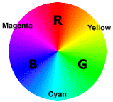
If we imagine the three primary colors red, green and blue
placed equally apart on a color wheel, all the other colors of the spectrum can
be created by mixes between any two of the primary colors. For example, the
printer's colors known as Magenta, Yellow, and Cyan are mid-way between Red and
Blue, Red and Green and Blue and Green respectively.
This diagram is called the color wheel, and any particular
spot on the wheel from 0 to 360 degrees is referred to as a hue, which
specifies the specific tone of color. "Hue" differsslightly from "color"
because a color can have saturation or brightness as well as a hue.

Saturation is the intensity of a hue from gray tone (no
saturation) to pure, vivid color (high saturation).

Brightness is the relative lightness or darkness of a
particular color, from black (no brightness) to white (full brightness).
Brightness is also called Lightness in some contexts.
2.6. PRIMARY COLOURS
It is a useful fact that the huge variety of colours that can
be perceived by humans can all be produced simply by adding together
appropriate amounts of red, blue and green colours. These colours are known as
the primary colours. Thus in most image processing applications, colours are
represented by specifying separate intensity values for red, green and blue
components. This representation is commonly referred to as RGB.
The primary colour phenomenon results from the fact that
humans have three different sorts of colour receptors in their retinas which
are each most sensitive to different visible light wavelengths.
The primary colours used in painting (red, yellow and blue)
are different. When paints are mixed, the `addition' of a new colour paint
actually subtracts wavelengths from the reflected visible light.
Colour Images
It is possible to construct (almost) all visible colours by
combining the three primary colours red, green and blue, because the human eye
has only three different colour receptor, each of them sensible to one of the
three colours. Different combinations in the stimulation of the receptors
enable the human eye to distinguish approximately 350,000 colours. A
RGB colour image is a multi-spectral image with one band for each colour red,
green and blue, thus producing a weighted combination of the three primary
colours for each pixel.
A full 24-bit colour image contains one 8-bit value for each
colour, thus being able to display different colours. However, it is
computationally expensive and often not necessary to use the full 24-bit to
store the colour for each pixel. Therefore, the colour for each pixel is often
encoded in a single byte, resulting in a 8-bit colour image. The process of
reducing the colour representation from 24-bits to 8-bits, known as colour
quantization, restricts the number of possible colours to 256. However, there
is normally no visible difference between a 24-colour image and the same image
displayed with 8 bits. A 8-bit colour images are based on colourmaps, which are
look up tables taking the 8 bit pixel value as index and providing an
output value for each colour.
RGB and Colourspaces
A colour perceived by the human eye can be defined by a linear
combination of the three primary colours red, green and blue. These three
colours form the basis for the RGB-colourspace. Hence, each perceivable colour
can be defined by a vector in the 3-dimensional colourspace. The intensity is
given by the length of the vector, and the actual colour by the two angles
describing the orientation of the vector in the colourspace.
The RGB-space can also be transformed into other coordinate
systems, which might be more useful for some applications. In this coordinate
system, a colour is described with its intensity, hue (average wavelength) and
saturation (the amount of white in the colour). This colour space makes it
easier to directly derive the intensity and colour of perceived light and is
therefore more likely to be used by human beings.
24-bit Colour Images
Full RGB colour requires that the intensities of three colour
components be specified for each and every pixel. It is common for each
component intensity to be stored as an 8-bit integer, and so each pixel
requires 24 bits to completely and accurately specifies its colour. Image
formats that store full 24 bits to describe the colour of each and every pixel
are therefore known as 24-bit colour images.
Using 24 bits to encode colour information allows different
colours to be represented, and this is sufficient to cover the full range of
human colour perception fairly well.[14]
The term 24-bit is also used to describe monitor displays that
use 24 bits per pixel in their display memories, and which are hence capable of
displaying a full range of colours.
There are also some disadvantages to using 24-bit images.
Perhaps the main one is that it requires three times as much memory, disk space
and processing time to store and manipulate 24-bit colour images as compared to
8-bit colour images. In addition, there is often not much point in being able
to store all those different colours if the final output device (e.g.
screen or printer) can only actually produce a fraction of them. Since it is
possible to use colourmaps to produce 8-bit colour images that look almost as
good, at the time of writing 24-bit displays are relatively little used.
However it is to be expected that as the technology becomes cheaper, their use
in image processing will grow.
2.7. MULTI-SPECTRAL
IMAGES
A multi-spectral image is a collection of several monochrome
images of the same scene, each of them taken with a different sensor. Each
image is referred to as a band. A well known multi-spectral (or
multi-band image) is a RGB colour image, consisting of a red, a green and a
blue image, each of them taken with a sensor sensitive to a different
wavelength. In image processing, multi-spectral images are most commonly used
for Remote Sensing applications. Satellites usually take several images from
frequency bands in the visual and non-visual range. Landsat 5, for
example, produces 7 band images with the wavelength of the bands being between
450 and 1250 nm.
All the standard single-band image processing operators can
also be applied to multi-spectral images by processing each band separately.
For example, a multi-spectral image can be edge detected by finding the edges
in each band and than ORing the three edge images together. However, we would
obtain more reliable edges, if we associate a pixel with an edge based on its
properties in all three bands and not only in one.
To fully exploit the additional information which is contained
in the multiple bands, we should consider the images as one multi-spectral
image rather than as a set of monochrome greylevel images. For an image with
k bands, we then can describe the brightness of each pixel as a point
in a k-dimensional space represented by a vector of length
k.
Special techniques exist to process multi-spectral images. For
example, to classify a pixel as belonging to one particular region, its
intensities in the different bands are said to form a feature vector
describing its location in the k-dimensional feature space. The
simplest way to define a class is to choose a upper and lower
threshold for each band, thus producing a k-dimensional `hyper-cube'
in the feature space. Only if the feature vector of a pixel points to a
location within this cube, is the pixel classified as belonging to this class.
A more sophisticated classification method is described in the corresponding
worksheet.
The disadvantage of multi-spectral images is that, since we
have to process additional data, the required computation time and memory
increase significantly. However, since the speed of the hardware will increase
and the costs for memory decrease in the future, it can be expected that
multi-spectral images will become more important in many fields of computer
vision.
2.8. LOOK UP TABLES AND
COLOURMAPS
Look Up Tables or LUTs are fundamental to many
aspects of image processing. An LUT is simply a table of cross-references
linking index numbers to output values. The most common use
is to determine the colours and intensity values with which a particular image
will be displayed, and in this context the LUT is often called simply a
colourmap.
The idea behind the colourmap is that instead of storing a
definite colour for each pixel in an image, for instance in 24-bit RGB format,
each pixel's value is instead treated as an index number into the colourmap.
When the image is to be displayed or otherwise processed, the colourmap is used
to look up the actual colours corresponding to each index number. Typically,
the output values stored in the LUT would be RGB colour values.
There are two main advantages to doing things this way.
Firstly, the index number can be made to use fewer bits than the output value
in order to save storage space. For instance an 8-bit index number can be used
to look up a 24-bit RGB colour value in the LUT. Since only the 8-bit index
number needs to be stored for each pixel, such 8-bit colour images take up less
space than a full 24-bit image of the same size. Of course the image can only
contain 256 different colours (the number of entries in an 8-bit LUT), but this
is sufficient for many applications and usually the observable image
degradation is small.
Secondly the use of a colour table allows the user to
experiment easily with different colour labeling schemes for an image.
One disadvantage of using a colourmap is that it introduces
additional complexity into an image format. It is usually necessary for each
image to carry around its own colourmap, and this LUT must be continually
consulted whenever the image is displayed or processed.
Another problem is that in order to convert from a full colour
image to (say) an 8-bit colour image using a colour image, it is usually
necessary to throw away many of the original colours, a process known as colour
quantization. This process is lossy, and hence the image quality is degraded
during the quantization process.
Additionally, when performing further image processing on such
images, it is frequently necessary to generate a new colourmap for the new
images, which involves further colour quantization, and hence further image
degradation.
As well as their use in colourmaps, LUTs are often used to remap
the pixel values within an image. This is the basis of many common image
processing point operations such as thresholding, gamma correction and contrast
stretching. The process is often referred to as anamorphosis.
2.9. LUMINOUS INTENSITY
In photometry, luminous intensity is a measure of the
wavelength-weighted power emitted by a light source in a particular direction,
based on the luminosity function, a standardized model of the sensitivity of
the human eye. The SI unit of luminous intensity is the candela (cd), an SI
base unit. Photometry deals with the measurement of visible light as perceived
by human eyes. The human eye can only see light in the visible spectrum and has
different sensitivities to light of different wavelengths within the spectrum.
When adapted for bright conditions (photopic vision), the eye is most sensitive
to greenish-yellow light at 555 nm. Light with the same radiant intensity
at other wavelengths has a lower luminous intensity. The curve which measures
the response of the human eye to light is a defined standard, known as the
luminosity function. This curve, denoted V(ë) , is based on an
average of widely differing experimental data from scientists using different
measurement techniques. For instance, the measured responses of the eye to
violet light varied by a factor of ten.
Luminous intensity should not be confused with another
photometric unit, luminous flux, which is the total perceived power emitted in
all directions. Luminous intensity is the perceived power per unit solid
angle. Luminous intensity is also not the same as the radiant intensity,
the corresponding objective physical quantity used in the measurement science
of radiometry.
Units
One candela is defined as the luminous intensity of a
monochromatic 540 THz light source that has a radiant intensity of
1/683 watts per steradian, or about 1.464 mW/sr. The 540 THz
frequency corresponds to a wavelength of about 555 nm, which is green
light near the peak of the eye's response. Since there are about
12.6 steradians in a sphere, the total radiant intensity would be about
18.40 mW, if the source emitted uniformly in all directions. A typical
candle produces very roughly one candela of luminous intensity.
In 1881, Jules Violle proposed the Violle as a unit
of luminous intensity, and it was notable as the first unit of light intensity
that did not depend on the properties of a particular lamp. It was superseded
by the candela in 1946.[15]
Intensity Histogram
In an image processing context, the histogram of an image
normally refers to a histogram of the pixel intensity values. This histogram is
a graph showing the number of pixels in an image at each different intensity
value found in that image. For an 8-bit greyscale image there are 256 different
possible intensities, and so the histogram will graphically display 256 numbers
showing the distribution of pixels amongst those greyscale values. Histograms
can also be taken of colour images either individual histograms of red, green
and blue channels can be taken, or a 3-D histogram can be produced, with the
three axes representing the red, blue and green channels, and brightness at
each point representing the pixel count. The exact output from the operation
depends upon the implementation it may simply be a picture of the required
histogram in a suitable image format, or it may be a data file of some sort
representing the histogram statistics.[15]
The working operation.
The operation is very simple. The image is scanned in a single
pass and a running count of the number of pixels found at each intensity value
is kept. This is then used to construct a suitable histogram.
Binary Images
Binary images are images whose pixels have only two possible
intensity values. They are normally displayed as black and white. Numerically,
the two values are often 0 for black, and either 1 or 255 for white. Binary
images are often produced by thresholding a greyscale or colour image, in order
to separate an object in the image from the background. The colour of the
object (usually white) is referred to as the foreground colour. The
rest (usually black) is referred to as the background colour. However,
depending on the image which is to be thresholded, this polarity might
be inverted, in which case the object is displayed with 0 and the background is
with a non-zero value.
Some morphological operators assume a certain polarity of the
binary input image so that if we process an image with inverse polarity the
operator will have the opposite effect. For example, if we apply a closing
operator to a black text on white background, the text will be opened.
Intensity of images.
Intensity images measure the amount of light impinging on a
photosensitive device. The input to the photosensitive device, typically a
camera, is the incoming light, which enters the camera's lens and hits the
image plane. In a digital camera, the physical image plane is an array which
contains a rectangular grid of photosensors, each sensitive to light intensity.
The output of the array is a continuous electric signal, the video signal. The
video signal is sent to an electronic device called frame grabber, where it is
digitised into a 2D rectangular array of integer values and stored in a memory
buffer.
The interpretation of an intensity image depends strongly on
the characteristics of the camera called the camera parameters. The parameters
can be separated into extrinsic and intrinsic parameters. The extrinsic
parameters transform the camera reference frame to the world reference frame.
The intrinsic parameters describe the optical, geometric and digital
characteristics of the camera. One parameter, for example, can describe the
geometric distortion introduced by the optics.
2.10. GAUSSIAN
SMOOTHING
The Gaussian smoothing operator is a 2-D convolution operator
that is used to `blur' images and remove detail and noise. In this sense it is
similar to the mean filter, but it uses a different kernel that represents the
shape of a Gaussian (`bell-shaped') hump. This kernel has some special
properties which are detailed below.
The idea of Gaussian smoothing is to use this 2-D distribution
as a `point-spread' function, and this is achieved by convolution. Since the
image is stored as a collection of discrete pixels we need to produce a
discrete approximation to the Gaussian function before we can perform the
convolution. In theory, the Gaussian distribution is non-zero everywhere, which
would require an infinitely large convolution mask, but in practice it is
effectively zero more than about three standard deviations from the mean, and
so we can truncate the mask at this point.[10]
2.11. FACE
IDENTIFICATION.
Face identification is very important in security,
surveillance and telecommunication applications. The proposed algorithm will be
used for face tracking in video surveillance system. In most cases the quality
and resolution of the recorded image-segments is poor and hard to identify a
face. For this reason, surveillance projects often use additional zooming
cameras to focus on region of interests. Disturbing effects might distort
recordings such as variations in illuminations, in pose or occlusions. Due to
the acquisition conditions the size of the face images is smaller (sometimes
much smaller) than the input image size in most of the existing face
recognition systems. For example, the valid face region could be as small as
15×15 pixels, whereas the face images used in still image based systems
are
at least 128 ×128 . Small-size images not only make the
recognition task difficult, but also affect the accuracy of face
segmentation.
In our approach we assume that the human head is detected and
localized. The task is divided into the following sub-tasks. First some
features are extracted to estimate the procession of the picture .Than the
digital image is transformed to create edges on the boundary of digital image,
in which the face is surrounded and scaled to a standard size. At last
searching the most similar face in a database makes the identification of
face.
CHAPTER 3. RESEARCH
METHODOLOGY.
This chapter deals with method used in conducting this project,
the materials and equipments used, including origin and standard
specifications.
3.1. METHOD USED AND
SOFTWARE DEVELOPMENT.
In order to accomplish this task, general methods and techniques
were used to collect data for this project as primary as well as secondary data
collection.
Secondary data correction.
Secondary data was corrected from published materials related to
the topic.
These include:
Book class notes and online information by visiting some websites
on the internet.
Library search was used to find background of digital image
processing of our project.
Websites consultancies: the main websites were
http://www.nacs.uci.edu/dcslib/matlab/matlabv60/help/toolbox/images/bwunpack.html
and
http://www.cogs.susx.ac.uk/courses/compvis/index/html
Primary data collection.
The study guide utilizes an extensive conversation containing
edge detection objectives. This conversation was done between researchers and
supervisor; also it was between researchers and class mast.
Data analysis.
After getting information about this project; we decided to use
software called «MATLAB version 6.5»(MATLAB 6p5) to achieve our main
objectives in this research.
3.1.1. DEFINITION OF
MATLAB.
MATLAB (MATrix LABoratory) is a programming language for
technical computing from the math works, Natick, MA. It is used for a wide
variety of scientific and engineering calculation, especially for automatic
control and signal processing. Matlab runs on windows, Mac and a variety of
unit based systems Developed by Cleve Moler in the late of 1970's and based on
the original LINPACK and EISPACK FORTRAN libraries, it was initially used for
factoring matrices and solving linear equations. Moler commercialized the
product with two colleagues in 1984. MATLAB is also noted for its extensive
graphics capabilities.[11]
Starting mat lab
To start MATLAB, you can use any of these methods.
Double-click on the MATLAB icon (called a "shortcut") that the
installer creates on your desktop.

Click on the Start button, select Programs, and click on the
MATLAB 6.5 entry. Select MATLAB 6.5 from this menu.
Using Windows Explorer, open your top-level MATLAB
installation directory and double-click on the shortcut to the MATLAB
executable, MATLAB 6.5.
Setting your initial current directory
By default, when you start MATLAB using the shortcut the
installer puts on your desktop, the initial current directory is the
$MATLAB\work directory, where $MATLAB represents the name of your installation
directory. The \work directory is a good place to store the M-files you modify
and create because the MATLAB uninstaller does not delete the \work directory
if it contains files. You can, however, use any directory as your MATLAB
initial current directory. To specify another directory as your initial current
directory, right-click on the MATLAB shortcut that the installer creates on
your desktop and select the Properties option. Specify the name of the
directory in the Start in field.
Setting up matlab environment options
To include welcome messages, default definitions, or any
MATLAB expressions that you want executed every time MATLAB is invoked, create
a file named startup.m in the $MATLAB\toolbox\local directory. MATLAB executes
this file each time it is invoked.
Configuring certain products
Certain products require additional configuration. The
following table lists these products and the commands used to configure them.
If you installed any of these products, see the documentation for that product
for detailed configuration information.
|
PRODUC
|
COMMAND
|
|
MATLAB Notebook
|
Notebook-setup
|
|
MATLAB Runtime server
|
Rtsetup
|
|
Real-Time Windows Target
|
rtwintgt -setup
|
Table 3.1.a: shows products and the
commands used to configure them.
Excel link versions
By default, Excel Link (a separately orderable product)
supports two versions of Excel. This table lists which Excel Link files to use
with each Excel version. Use the appropriate files for your version of Excel.
You can find these files in the $MATLAB\toolbox\exlink subdirectory.
|
EXCEL VERSION
|
EXCEL LINK FILE
|
|
Excel 97 (Default)
|
excllink.xla ExliSamp.xls
|
|
Excel 7
|
excllink95.xla ExliSamp95.xls
|
Table 3.1.b: shows Excel
files to use with each Excel version.
Finding information about matlab
After successfully installing MATLAB, you are probably eager
to get started using it. This list provides pointers to sources of information
and other features you may find helpful in getting started with MATLAB.
|
TASKS
|
DESCRIPTION
|
|
To get an overview of MATLAB and its capabilities
|
Read the Release Notes documentation
|
|
To find out what's new in this release
|
Read the Release Notes documentation
|
|
To start a product or run one of the demonstration programs
|
Use the Launch Pad in the MATLAB desktop
|
|
To get information about specific MATLAB feature
|
Choose the Help item in the MATLAB menu bar to view reference and
tutorial information in hyperlinked HTML form.
|
|
To get help with specific questions you can't find answered in
the documentation
|
Go to the Math Works Web site (www.mathworks.com), click on
Support, and use the Technical Support solution search area to find more
information
|
Table 3.1.c: shows finding information about
matlab.
3.1.3. FUNCTION USED BY
MATLAB.
MATLAB standards functions are so many but we need this:
USER DEFINED FUNCTION.
1. graythresh function: is the function used to
determine a threshold value.
2. strel function: is a function used to
disappear the linear gaps if the sobel image is dilated using linear
structuring elements.
3. imdilate function: is the function used to
dilate the binary gradient mask using the vertical structuring element followed
by the horizontal structuring element.
4. imfill function: is the function used to fill
the interior holes(gaps) of image.
5. imclearboarder function: is used to remove
the connected object to the border of the image. We create the diamond
structuring element using the strel function.
6. bwperim function: is the function used to
place an outline around the segmented object.
7. BW = edge (I,'sobel'): specifies the Sobel
method.
8. BW = edge (I,'sobel',thresh): specifies
the sensitivity threshold for the Sobel method edge ignores all edges that are
not stronger than thresh. If you do not specify thresh, or if thresh is empty
([]), edge chooses the value automatically.
MATLAB STANDARD FUNCTION.
MATLAB is a powerful programming language as well as an
interactive computational environment. Files that contain code in the MATLAB
language are called M-files. You create M-files using a text editor, then use
them as you would any other MATLAB function or command.
There are two kinds of M-files:
Scripts, which do not accept input arguments
or return output arguments. They operate on data in the workspace.
Functions, which can accept input arguments
and return output arguments. Internal variables are local to the function.
If you're a new MATLAB programmer, just create the M-files
that you want to try out in the current directory. As you develop more of your
own M-files, you will want to organize them into other directories and personal
toolboxes that you can add to your MATLAB search path.
M-FILE SCRIPTS.
SCRIPTS are the simplest kind
of M-file because they have no input or output arguments. They are useful for
automating series of MATLAB commands, such as computations that you have to
perform repeatedly from the command line.
THE BASE WORKSPACE
Scripts share the base workspace with your interactive MATLAB
session and with other scripts. They operate on existing data in the workspace,
or they can create new data on which to operate. Any variables that scripts
create remain in the workspace after the script finishes so you can use them
for further computations. You should be aware, though, that running a script
can unintentionally overwrite data stored in the base workspace by commands
entered at the MATLAB command prompt.
Simple script example
These statements calculate rho for several trigonometric
functions of theta, then create a series of polar plots:
% An M-file script to produce % Comment lines
% "flower petal" plots
theta =
-pi:0.01:pi; % Computations
rho(1,:) = 2 * sin(5 * theta) .^ 2;
rho(2,:) = cos(10 * theta) .^ 3;
rho(3,:) = sin(theta) .^ 2;
rho(4,:) = 5 * cos(3.5 * theta) .^ 3;
for k = 1:4
polar(theta, rho(k,:)) %
Graphics output
pause
end
Try entering these commands in an M-file called petals.m. This
file is now a MATLAB script. Typing petals at the MATLAB command line executes the statements in the script.
M-FILE FUNCTION
FUNCTIONS are program routines, usually implemented in
M-files, that accept input arguments and return output arguments. They operate
on variables within their own workspace. This workspace is separate from the
workspace you access at the MATLAB command prompt.
THE FUNCTION WORKSPACE
Each M-file function has an area of memory, separate from the MATLAB base workspace, in
which it operates. This area, called the function workspace, gives each
function its own workspace context.
While using MATLAB, the only variables you can access are
those in the calling context, be it the base workspace or that of another
function. The variables that you pass to a function must be in the calling
context, and the function returns its output arguments to the calling workspace
context. You can, however, define variables as global variables explicitly,
allowing more than one workspace context to access them. You can also evaluate
any MATLAB statement using variables from either the base workspace or the
workspace of the calling function using the evalin function.
Simple function
example
The average function is a simple M-file that calculates the
average of the elements in a vector:
function y = average(x)
% AVERAGE Mean of vector elements.
% AVERAGE(X), where X is a vector, is the mean of vector
% elements. Nonvector input results in an error.
[m,n] = size(x);
if (~((m == 1) | (n == 1)) | (m == 1 & n == 1))
error('Input must be a vector')
end
y = sum(x)/length(x); % Actual computation
Try entering these commands in an
M-file called average.m. The average function accepts a single input argument
and returns a single output argument. To call the average function, enter
z = 1:99;
average(z)
ans =
50
TYPES OF M-FILES FUNCTION
Many functions are used. For instance, the following are the used
functions:
The Primaty M-File Functions: is the first function in an
M-file and typically contains the main program. Primary functios have a wide
scope, the primary function can be invoked from outside of their M-File(from
the matlab command line or from function in other file).
Subfunctions: act as subroutines to the main
function. You can also use them to define multiple functions within a single
M-file.
Nested Functions: are functions defined within another
function. They can help to improve the readability of your program and also
give you more flexible access to variables in the M-file.
Overloaded functions: are useful when you need to create a
function that responds to different types of inputs accordingly. They are
similar to overloaded functions in any object-oriented language.
3.1.4. COMMANDS USED.
MATLAB has so many commands, but we need this:
0. Imread(): this command is used for reading an
image. Within the parentheses, you type the name of an image file you wish to
read. Put the filename within the single quotes.
1. Imshow(): this command is used to display an
image represented as the matrix.
2. rgb2gray(): this command is used to
convert between RGB format to intensity (grayscale) format.
3. figure: this command can be used to create a
new current figure for the display. 4. Imdilate: this command
is used to dilate the image.
5. figure(n): will check whether the figure n
exists, if it switches the focus to it, otherwise a new window is created.
6. Double: convert a matrix to the
double-precision floating- point format.
7. Imagesc ( ): t his command is used to display
an image
8. Edge: is command used to create the binary
gradient mask.
9. save x and load x: these commands are used
to load and save variables in MATLAB. Once you have read a file, you probably
convert it into an intensity image (a matrix) and work with this matrix; this
matrix is represented by the variable x.
3.1.5. SYMBOLES USED.
1. ASTERISK (*): An asterisk in a
filename specification is used as a wildcard specified.
2. COLON (:) the colon operator
generates a sequence of numbers that you can use in creating or indexing into
arrays.
3. COMMA (,): comma is used to
separate the following types of elements
4. DOT (.): the single dot operator
has the following different uses in MATLAB.
5. DOT-DOT (..):two dots in sequence
refer to the parent of the current directory.
6. EXCLAMATION POINT (!): The
exclamation point precedes operating system commands that you want to execute
from within MATLAB.
7. PARENTHESES ( ): Parentheses are
used mostly for indexing into elements of an array or for specifying arguments
passed to a called function.
8. PERCENT (%): The percent sign
is most commonly used to indicate no executable text within the body of a
program. This text is normally used to include comments in your code. Some
functions also interpret the percent sign as a conversion specifier.
9. SEMICOLON (;): The semicolon
can be used to construct arrays, suppress output from a MATLAB command, or to
separate commands entered on the same line. Bt the way, semicolon prevents
showing the result of the program line in workspace. This is handily especially
with image.
10. SINGLE QUOTES (' '): Single
quotes are the constructor symbol for MATLAB character arrays.
11. SPACE CHARACTER: The space
character serves a purpose similar to the comma in that it can be used to
separate row elements in an array constructor, or the values returned by a
function.
12. SLASH AND BACKSLASH / \: the slash (/) and backslash (\)
characters separate the elements of a path or directory string. On
Windows-based systems, both slash and backslash have the same effect. On
UNIX-based systems, you must use slash only.
On a Windows system, you can use either backslash or slash:
dir([matlabroot '\toolbox\matlab\elmat\shiftdim.m'])
dir([matlabroot '/toolbox/matlab/elmat/shiftdim.m'])
On a UNIX system, use only the forward slash:
dir([matlabroot '/toolbox/matlab/elmat/shiftdim.m'])
13. SQUARE BLACKETS [ ]: Square
brackets are used in array construction and concatenation, and also in
declaring and capturing values returned by a function.
14. CURLY BRACES { }: Use curly
braces to construct or get the contents of cell arrays,
3.1.6. TO WRITE MATLAB
PROGRAMS
MATLAB programs can be written straight to command line (1),
or in m-files. M-files are created by (2), or writing edit
functionName on command line (1). Created files are stored as filename
to current directory, which you can change in (3). You can, for example in case
of a shared computer in laboratory exercises, create a temp directory
under work for keeping your files organized.
FUNCTIONS AND SCRIPTS.
Script is simple M-file that executes all lines as
they were written in the command line. It has no «headers» or
anything, just plain program lines. Scripts see all variables created in
Command line (i.e. workspace) and vice versa.
Functions are «advanced scripts», that take can take
parameters and can produce outputs. Examples of both a script and a function
are given bellow:
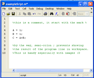
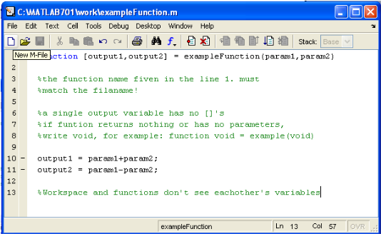
To use a script write scriptName on command line.
To use a function, write [output1,outpu2,...] =
functionName(param1, param2) on command line.
In case of single output, drop the []'s. MATLAB has
numerous functions to help your work. You can find out how to use a function by
typing help functionName on command line.
3.1.7. TO END A
PROGRAM.
After writing a program; you have to end it or to finish it in
other to run the writing program. To do this, you type «end» at the
final line of your program.
3.1.8. ACCESS TO
IMPLEMENTATION DETAILS
MATLAB provides many functions for image processing and other
tasks. Most of these functions are written in the MATLAB language and are
publicly readable as plain text files. Thus the implementation details of these
functions are accessible and open to scrutiny. The defense can examine the
processing used in complete detail, and any challenges raised can be responded
to in an informed way by the prosecution. This makes MATLAB very different from
applications, such as Photoshop.
It should be noted that some MATLAB functions couldn't be
viewed. These are generally lower level functions that are computationally
expensive and are hence provided as 'builtin' functions running as native code.
These functions are heavily used and tested and can be relied on with
considerable confidence.
3.1.9. FUNDAMENTALS ON
MATLAB.
A digital image is composed of pixels, which can be
thought of as small dots on the screen. A digital image is an instruction of
how to colour each pixel. We will see in detail later on how this is done in
practice. A typical size of an image is 512-by-512 pixels. Later on in the
course you will see that it is convenient to let the dimensions of the image to
be a power of 2. For example, 29=512. In the general case we say
that an image is of size m-by-n if it is composed of
m pixels in the vertical direction and n pixels in the
horizontal direction.
Let us say that we have an image on the format 512-by-1024
pixels. This means that the data for the image must contain information about
524288 pixels, which requires a lot of memory! Hence, compressing images is
essential for efficient image processing.
APPLICATION OF MATLAB.
The matlab has more application:
Mathematical operation
v Vectors
v Matrices and Matrix operations
v Solving systems of linear equations
v Plotting
v Curve fitting, Interpolation
v MATLAB commands
v Preparing data files and M files
THE USE OF MATLAB.
MATLAB may not be as user friendly as an application like
Photoshop, however, being a general purpose programming language it provides
many important advantages for forensic image processing. It ensures the image
processing steps used are completely documented, and hence can be replicated.
In general, the source code for all image processing functions are accessible
for scrutiny and test. It allows one to ensure numerical precision is
maintained all the way through the enhancement process.
Image processing algorithms available under MATLAB are likely
to be more advanced than those available from other image processing
applications.
3.1.10. IMAGE TYPES AND
DATA CLASSES
MATLAB supports intensity images (including binary images),
indexed images, and color images. Most of this class will involve intensity
images, in which each pixel is a scalar measure of light by a detector. Binary
images have only values 0 or 1 for 'no light' or 'light'. Binary pixel values
can be represented with one bit and packed into bytes.
Intensity images with more precision can use integer data of
various lengths or floating point data of various lengths. Typically, we will
use uint8 (unsigned 8-bit integers) or double (double-precision floating point
numbers).
MATLAB has functions for converting the data types of
images. It is important to understand the mathematics of these
conversions.
Image Indexing
The value of a single pixel in an image is indexed as:
p(m,n)
Multiple pixels can be indexed with a vector as:
p([1 3],1) which selects pixels p(1,1) and p(3,1).
Multiple pixels also can be indexed using a range. The
first row is all pixels with row index 1 and any column index:
p(1,1:N) The notation 1:N indicates all indexes from 1 to N.
The notation can contain a step value, e.g., 1::2:5 indicates
indexes 1, 3, 5.
The keyword end can be used to indicate the last index. The range
operator by itself, :, indicates the full range, from 1 to end either of a
dimension or of the whole matrix.
Standard Arrays
MATLAB has standard arrays for creating arrays of a defined
size with zeros, ones, true, false, or random values. For example:
p = zeros(M,N);
Builtin Functions
MATLAB has many useful builtin functions listed in Appendix A
of the text book. For example:
max(p(:))
Gives the largest value in the matrix.
Note, given matrix p, max(p) treats the matrix as an array of
column vectors and returns a vector of the largest value in each column.
Operators
MATLAB has builtin arithmetic, relational, and logical
operators.
Two images can be added so that the output value at each pixel
is the sum of the values of the corresponding input pixels. For
example:
r = p+q;
which also can be written:
r = plus(p,q);
The operands can be scalars, vectors, or matrices.
The array and matrix arithmetic operations are done in double
precision floating point. MATLAB also provides operations which support
integer arithmetic, e.g., imadd and immultiply,
For multiplication and some other operations, MATLAB has two
types of arithmetic operations: array arithmetic operations which perform the
operation on corresponding pixels of the input images and matrix arithmetic
operations which perform matrix arithmetic.
Array multiplication is:
r = p.*q;
or
r = times(p,q);
Matrix multiplication is:
r = p*q;
or
r = mtimes(p,q);
3.1.11. IMAGE FORMATS SUPPORTED BY MATLAB
The following image formats are supported by Matlab:
BMP, HDF, JPEG, PCX, XWD and TIFF.
Most images you find on the Internet are JPEG-images which is
the name for one of the most widely used compression standards for images. If
you have stored an image you can usually see from the suffix what format it is
stored in. For example, an image named myimage.jpg is stored in the JPEG format
and we will see later on that we can load an image of this format into
Matlab.
WORKING FORMATS IN MATLAB
If an image is stored as a JPEG-image on your disc we first
read it into Matlab. However, in order to start working with an image, for
example perform a wavelet transform on the image, we must convert it into a
different format. This section explains four common formats.
Intensity image (gray scale image)
This is the equivalent to a "gray scale image" and this is the
image we will mostly work with in this course. It represents an image as a
matrix where every element has a value corresponding to how bright/dark the
pixel at the corresponding position should be colored. There are two ways to
represent the number that represents the brightness of the pixel: The double
class (or data type). This assigns a floating number ("a number with decimals")
between 0 and 1 to each pixel. The value 0 corresponds to black and the value 1
corresponds to white. The other class is called uint8, which assigns an integer
between 0 and 255 to represent the brightness of a pixel. The value 0
corresponds to black and 255 to white. The class uint8 only requires roughly
1/8 of the storage compared to the class double. On the other hand, many
mathematical functions can only be applied to the double class. We will see
later how to convert between double and uint8.
Binary image
This image format also stores an image as a matrix but can
only color a pixel black or white (and nothing in between). It assigns a 0 for
black and a 1 for white.
Indexed image
This is a practical way of representing color images. (In this
course we will mostly work with gray scale images but once you have learned how
to work with a gray scale image you will also know the principle how to work
with color images.) An indexed image stores an image as two matrices. The first
matrix has the same size as the image and one number for each pixel. The second
matrix is called the color map and its size may be different from the image.
The numbers in the first matrix is an instruction of what
number to use in the color map matrix.
RGB image
This is another format for color images. It represents an
image with three matrices of sizes matching the image format. Each matrix
corresponds to one of the colors red, green or blue and gives an instruction of
how much of each of these colors a certain pixel should use.
Multiframe image
In some applications we want to study a sequence of images.
This is very common in biological and medical imaging where you might study a
sequence of slices of a cell. For these cases, the multiframe format is a
convenient way of working with a sequence of images. In case you choose to work
with biological imaging later on in this course, you may use this format.
3.1.11. CONVERSION BETWEEN
DIFFERENT FORMATS
The following table shows how to convert between the different
formats given above. All these commands require the Image processing
toolbox!
Image format conversion.
Within the parenthesis you type the name of the image you wish to
convert.
|
Operation:
|
Matlab command:
|
|
Convert between intensity/indexed/RGB formats to binary
format.
|
dither()
|
|
Convert between intensity format to indexed format.
|
gray2ind()
|
|
Convert between indexed format to intensity format.
|
ind2gray()
|
|
Convert between indexed format to RGB format.
|
ind2rgb()
|
|
Convert a regular matrix to intensity format by scaling.
|
mat2gray()
|
|
Convert between RGB format to intensity format.
|
rgb2gray()
|
|
Convert between RGB format to indexed format.
|
rgb2ind()
|
Table 3.1.d: Shows conversion between different
formats.
The command mat2gray is useful if you have a matrix
representing an image but the values representing the gray scale range between,
let's say, 0 and 1000. The command mat2gray automatically re scales all entries
so that they fall within 0 and 255 (if you use the uint8 class) or 0 and 1 (if
you use the double class).
CONVERSION BETWEEN double AND uint8
When you store an image, you should store it as a uint8 image
since this requires far less memory than double. When you are processing an
image (that is performing mathematical operations on an image) you should
convert it into a double. Converting back and forth between these classes is
easy.
I=im2double(I);
converts an image named I from uint8 to double.
I=im2uint8(I);
converts an image named I from double to uint8.
Conversions between Different Image
Types
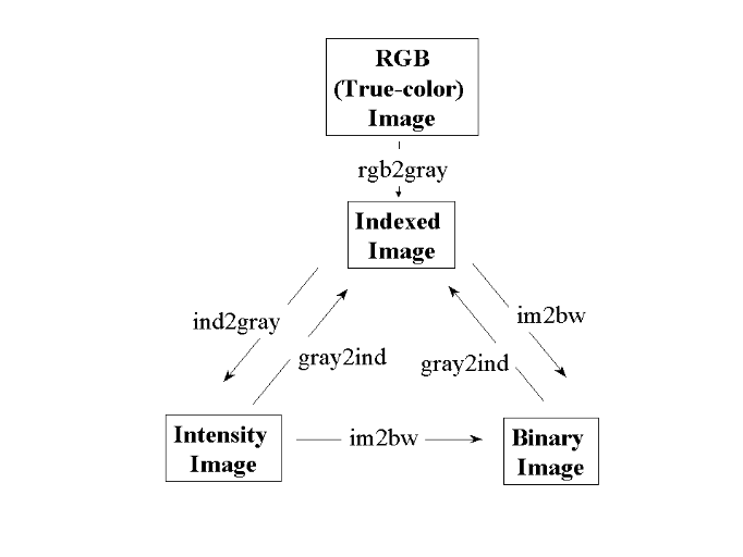
Figure 3.1: Conversion between different image
types.
3.2. EQUIPMENTS USED.
I n order to accomplish our project, we are used the
equipments such as digital computer in processing of the object(image) and
digital camera as the source of images. We can found more details of these
equipments in section 2.2 and section 2.3.
3.3. MATERIALS USED.
In conducting this research, we were used materials of images
like photos as samples.
The file formats of the used photos are:
JPEG means joint photograph expert graphics and BMP which means
bitmap format.
3.4. DETECTING AN OBJECT
USING IMAGE SEGMENTATION.
An object can be easily detected in an image if the object has
sufficient contrast from the background. We use edge detection and basic
morphology tools to detect a prostate cancer cell. To conduct this detection,
there are many steps to follow:
v Step 1: Read Image
v Step 2: Convert RGB to Gray
v Step 3: Detect Entire object
v Step 4: fill the gaps
v Step 5: Dilate the Image
v Step 6: Fill Interior Gaps
v Step 7: Remove Connected Objects on Border
v Step 8: Smooth the Object
STEP 1: READ IMAGE.
Read in 'filename.gpj', which is an image of a prostate cancer
filename.
I = imread('filename.jpg');
%filename is the name of the object to be detected and .jpg is
the file format of this image.
figure, imshow(I), title('original image'); % shows the
figure to be red.
STEP 2: CONVERT RGB TO GRAY
The image to be detected is the colour image, to detect it
correctly; we have to convert it into gray scale (intensity value) using the
command «rgb2gray».
rgb2gray(`filename.jpg');
newmap=rgb2gray(I);
figure, imshow(newmap), title(`gray image'); % shows the
converted figure.
STEP 3: DETECT ENTIRE OBJECT.
We will detect this object; another word for object detection
is segmentation. The object to be segmented differs greatly in contrast from
the background image. Changes in contrast can be detected by operators; that
calculate the gradient of an image. One way to calculate the gradient of an
image is the Sobel operator, which creates a binary mask using a user-specified
threshold value. We determine a threshold value using the graythresh function.
To create the binary gradient mask, we use the edge function.
BWs = edge (I, 'sobel', (graythresh(I) * .1)); % detects edges of
processed image.
% BWs means binary gradient mask
figure, imshow(BWs), title('binary gradient mask'); %shows the
binary gradient mask.
STEP 4: FILL GAPS
The binary gradient mask shows lines of high contrast in the
image. These lines do not quite delineate the outline of the object of
interest. Compared to the original image, you can see gaps in the lines
surrounding the object in the gradient mask. These linear gaps will disappear
if the Sobel image is dilated using linear structuring elements, which we can
create with the strel function.
se90 = strel ('line', 3, 90);
se0 = strel ('line', 3, 0);
STEP 5: DILATE THE IMAGE
The binary gradient mask is dilated using the vertical
structuring element followed by the horizontal structuring element. The
imdilate function dilates the image.
BWsdil = imdilate(BWs, [se90 se0]);
figure, imshow(BWsdil), title('dilated gradient mask');
STEP 6: FILL INTERIOR GAPS
The dilated gradient mask shows the outline of the cell quite
nicely, but there are still holes in the interior of the cell. To fill these
holes we use the imfill function.
BWdfill = imfill(BWsdil, 'holes');
figure, imshow(BWdfill), title('binary image with filled
holes');
STEP 7: REMOVE CONNECTED OBJECTS ON BORDER
(This step will be used when there are others object on the
border of the detected object). The object of interest has been successfully
segmented, but it is not the only object that has been found. Any objects that
are connected to the border of the image can be removed using the imclearborder
function. The connectivity in the imclearborder function was set to 4 to remove
diagonal connections.
BWnobord = imclearborder(BWdfill, 4);
STEP 8: SMOOTH THE OBJECT
Finally figure, imshow(BWnobord), title('cleared border
image');
, in order to make the segmented object look natural, we
smooth the object by eroding the image twice with a diamond-structuring
element. We create the diamond-structuring element using the strel function.
seD = strel('diamond',1);
BWfinal = imerode(BWnobord,seD);
BWfinal = imerode(BWfinal,seD);
figure, imshow(BWfinal), title('segmented image');
An alternate method for displaying the segmented object would
be to place an outline around the segmented object. The outline is created by
the bwperim function.
BWoutline = bwperim(BWfinal);
Segout = I;
Segout(BWoutline) = 255;
figure, imshow(Segout), title('outlined original image');
3.5. IMPLEMENTATION OF EDGE
DETECTION.
I n this section, implementation was based on two different
operators such as:
Sobel operators and Prewitt operators. These two operators are
used in writing program, which were basically used in processing of digital
images. Here is the whole program:
|
Writeable commands
|
Results obtained.
|
|
I=imread('dushime.jpg');
figure, imshow(I), title('original image');
|
|
|
rgb2gray('dushime.jpg');
newmap=rgb2gray(I);
figure, imshow(newmap),title('gray image');
|
|
|
BWs=edge(newmap, 'sobel', (graythresh(newmap) * .1));
figure, imshow(BWs), title('binary gradient');
|
|
|
Se90=strel('line', 3, 90);
Se0=strel('line', 3, 0);
BWsdil=imdilate(BWs, [Se90 Se0]);
figure, imshow(BWsdil), title('dilated gradient mask');
|
|
|
BWdfill=imfill(BWsdil,'holes');
figure, imshow(BWdfill), title('binary image with filled
holes');
|
|
|
BWnobord=imclearborder(BWdfill,4);
figure, imshow(BWnobord), title('cleared border image');
|
|
|
SeD=strel('diamond',1);
BWfinal=imerode(BWnobord,SeD);
BWfinal=imerode(BWfinal,SeD);
figure, imshow(BWfinal), title('segmented image');
|
|
|
BWoutline=bwperim(BWfinal);
segout=I;
segout(BWoutline) = 255;
figure, imshow(segout), title('outline original image');
end
|
|
The above program is used to process the JPEG format while the
following program is used to process the BMP format.
|
I=imread('nouvelle.bmp');
figure, imshow(I), title('original image');
|
|
|
rgb2gray('nouvelle.bmp');
newmap=rgb2gray(I);
figure, imshow(newmap),title('gray image');
|
|
|
BWs=edge(newmap, 'sobel', (graythresh(newmap) * .1));
figure, imshow(BWs), title('binary gradient');
|
|
|
Se90=strel('line', 3, 90);
Se0=strel('line', 3, 0);
BWsdil=imdilate(BWs, [Se90 Se0]);
figure, imshow(BWsdil), title('dilated gradient mask');
|
|
|
BWdfill=imfill(BWsdil,'holes');
figure, imshow(BWdfill), title('binary image with filled
holes');
|
|
|
BWnobord=imclearborder(BWdfill,4);
figure, imshow(BWnobord), title('cleared border image');
|
|
|
SeD=strel('diamond',1);
BWfinal=imerode(BWnobord,SeD);
BWfinal=imerode(BWfinal,SeD);
figure, imshow(BWfinal), title('segmented image');
|
|
|
BWoutline=bwperim(BWfinal);
segout=I;
segout(BWoutline) = 255;
figure, imshow(segout), title('outline original image');
end
|
|
PREWITT OPERATOR (EDGE DETECTOR).
|
% edge detection with prewitt operator
filename= 'NEW.bmp'; % the filename to be read
image = imread(filename);
Imshow(image); % display
|
|
|
rgb2gray('NEW.bmp');
newmap=rgb2gray(image);
figure, imshow(newmap),title('gray image');
|
|
|
axis('square');
colormap('gray');
sze=size(newmap);
rows = sze(1); cols = sze(2);
|
|
|
% apply prewitt
Prw_im=edge(newmap,'prewitt');
figure(2);
|
|
|
imagesc(Prw_im);
axis('square');
colormap('gray');
end
|
|
EDGE DETECTION WITH SOBEL
|
% edge detection with Sobel operator program
filename= 'NEw.bmp'; % the filename to be read
image = imread(filename);
figure,Imshow(image),title('original image'); % display
|
|
|
rgb2gray('NEW.bmp');
newmap=rgb2gray(image);
figure,imshow(newmap),title('gray image');
|
|
|
axis('square');
colormap('gray');
sze=size(newmap);
rows = sze(1); cols = sze(2);
|
|
|
% apply sobel
sob_im=edge(newmap,'sobel');
figure(2);
|
|
|
imagesc(sob_im);
axis('square');
colormap('gray');
end
|
|
COMPARISON FOR EDGE DETECTION BETWEEN SOBEL AND
PREWITT.
|
Writeable program
|
Obtainable result
|
|
% comparison for edge detection between Sobel & Prewitt
operators.
filename= 'NEW.bmp'; % the filename to be read
image = imread(filename);
figure, Imshow(image), title ('original imge') % display
|
|
|
rgb2gray('NEW.bmp');
newmap=rgb2gray(image);
figure, imshow(newmap),title('gray image');
|
|
|
axis('square');
colormap('gray');
sze=size(newmap);
rows = sze(1); cols = sze(2);
|
|
|
% apply prewitt
sob_im = edge(newmap,'sobel');
figure, imshow(sob_im), title ('sobel image');
|

Figure 3.5.a. sobel image
|
|
prw_im= edge(newmap,'Prewitt');
figure, imshow(prw_im), title('prewitt image');
|
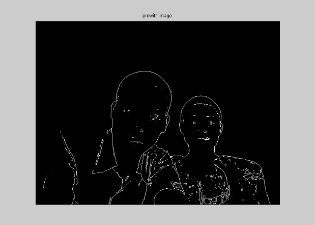
Figure 3.5.b. prewitt image.
|
|
dif_im=double(sob_im)- double(prw_im);
figure(2);
|
|
|
imagesc(dif_im);
axis('square');
colormap('gray');
end
|
|
CHAPTER 4. RESULTS AND
DISCUSSION.
4.1. RESULTS.
The basic requirement of this MATLAB program is to implement
edge detection. The Sobel and Prewitt edge detector can also be applied to
range the image (sampled picture) called Sobel figure and Prewitt figure. The
corresponding edge image has been detected and can nice separated from the
background.
Sobel edge detector.
The Sobel edge detection based on Sobel operator has the
advantages of emphasizing the central part of the edge. It places emphasis on
pixels that are closer to the center of the mask. Each direction of Sobel
operator is applied to the image. One image shows the vertical response and
other show the horizontal response. Purpose is to determine the existence and
location of edge in picture.
When the object containing sharp edges and its surface is
rather smooth, therefore could easily detect the boundary of the object without
getting any erroneous pixels.
For the object containing many fine depth variations on its
surface, applying the Sobel operator we can see that the intensity of many
pixels on surface is high as long as the actual edges. Once reason is that the
output of many edge pixels is greater than the maximum pixels values therefore
there is `cutoff' at 255.
To avoid this over flow we scale the range image by a factor
0.25 prior to edge detection and then normalize the output although the result
has improved significantly.
The Sobel operator is based on convolution in very small
neighborhood and work well for specific image only.
The many disadvantages of this edge detection is its
dependence on the size of object and sensitivity to noise.
The Sobel operator is very quick to computer and rather simple
to implement. It yields the best result. The Sobel operator is one of the most
commonly used edge detectors..
Prewitt edge detector
The Prewitt edge detector based on Prewitt operator
approximates the first derivatives. This operator does not place any pixels
that are closer to the center of the mask.
The Prewitt edge detector masks are one of the oldest and best
understood methods of detecting edges in image. Basically there two mask one
for detecting image derivatives in X and other one for detecting image
derivatives in Y. The results of Prewitt edge detection are thresholded in
order to produce a discrete set of edges. The direction of gradient mask is
given by the mask giving maximal response.
Comparison.
The sobel and Prewitt operators use the first derivative. They
have very simple calculation to detect edges and their orientation but they
have inaccurate detection sensitivity in case of noise because the subjective
evaluation of edge detection result images show that under noisy condition
Prewitt and Sobel operator have poor quality.
As we have seeing in the precession of digital images (in
chap.3); Prewitt and Sobel mark difference between them. The difference is that
Sobel edge detector marks a lot of number of pixels while the Prewitt edge
detector marks a few number of pixels.
Image file format used.
The processed picture has been saved in different file format.
The chosen file format can impact the clarity of picture. The following file
formats have been chosen in this work such as JPEG, BMP, PNG, and GIF. The
digital camera used when we shooted pictures offered JPEG setting, in order to
achieve uor objective we tried to put the taken pictures into different file
format using software that is able to convert them into the wanted format(e.g:
Microsoft office picture manager).
The processed done using both sobel and Prewitt operators. A
picture which is in JPEG file format when it is converted into other file
format the number of pixels are variable according to the used operator(sobel
or Prewitt).
When the picture is converted into GIF file format the sobel
operators shows high number of pixels than JPEG, but Prewitt operator shows few
number of pixels than the JPEG.
When the picture is converted into PNG file format, its
procession with sobel shows high number of pixels than JPEG, but the Prewitt
shows some number of number of pixels as JPEG. When a picture is converted into
BMP file format, its procession with sobel and Prewitt operators show the same
number of pixels as JPEG file format.
The following table shows the summary of above analysis:
|
Original format picture
(reference)
|
Format after conversion
|
Number of pixels
|
|
Sobel operator
|
Prewitt operator
|
|
JPEG
|
JPEG
|
same
|
Same
|
|
JPEG
|
PNG
|
High
|
Same
|
|
JPEG
|
GIF
|
High
|
Low
|
|
JPEG
|
BMP
|
same
|
Same
|
Table 4.1: shows comparison of number of pixels
between PNG, GIF, BMP file formats and JPEG file format.
Contrast and brightness.
As we know that : the term contrast refer to the amount of
color or gray scale differentiation that exist between various images features
in both analog and digital image while brightness is the relative lightness or
darkness of particular color from black to white. When a brightness of
processed picture is increased at high level and contrast in the normal
contrast of image's capturing, they were no pixels at the segmented image in
both operator s(sobel and Prewitt).
When brightness is reduced at low level and contrast remains
in the contrast of image's capturing, the unwanted pixels at segmented image
occurred because of the background and the object were changed when the
brightness was changed.
When contrast is increased at high level and brightness
remains in normal condition, the Prewitt operator shows the unwanted pixels
because there were no edges at segmented image and sobel operator shows us only
the background.
When contrast was reduced at low level and brightness remains in
its normal condition, pixels are available as the background remains
unchangeable, there is no noise in both the sobel and Prewitt operators.
When contrast and brightness are increased there are no pixels
on the face because the face tends to be as the background. But when both are
reduced at low level there are the unwanted pixels on the segmented image,
because pixels are located any where brightness is cleared.
Reducing contrast level and increasing brightness level no
pixels are shown on segmented image in both sobel and Prewitt operators while
reducing brightness level and increasing contrast level more pixels are shown
on brig area only.
The following table shows the summary of above analysis:
|
Contrast level
|
Brightness level
|
Observation on the output
|
|
Normal position of image's capturing
|
high
|
No pixels
|
|
Normal position of image's capturing
|
Low
|
Noise(unwanted pixels on segmented image)
|
|
High
|
Normal position of capturing of image
|
Background
|
|
Low
|
Normal position of capturing of image.
|
Pixels available
|
|
High
|
High
|
No pixels
|
|
Low
|
Low
|
Noise(unwanted pixels on segmented image)
|
|
High
|
Low
|
Pixels available on bright area
|
|
Low
|
High
|
No pixels
|
|
Normal position of image's capturing
|
Normal position of image's capturing
|
Pixels available
|
Table 4.2: shows the results based on variation
of contrast and brightness.
4.2. DISCUSSION.
The number of pixels in the picture depends on the resolution
of used digital camera; small resolution corresponds to less number of pixels
and high resolution results in more pixels.
The outlook of pixels on detected pictures depends on the
weight of each picture. When a picture has small weight i.e. brightness and
contast5 are at low level, pixels are not well seen. When a picture is being
zoomed out its weight increase and pixels are well seen.
If the picture contains sharp edges and its surface is rather
smooth, its boundaries could be detected easily without getting any erroneous
pixels.
CHAPTER 5. CONCLUSION AND
RECOMMENDATION.
5.1. CONCLUSION.
As it was tried to express on the beginning of this paper, the
main purpose of this project was intended to implement edge detection for
digital image.
There are several algorithms that are able to detect edges.
Our implementation was based on two edge detection operators
which are Sobel and Prewitt operators, for determination of existence and
location of edge in picture.
The Sobel operator yields the best result containing many
pixels on the image. It is very quick to computer and rather simple to
implement.
The Prewitt operator yields the result containing fewer pixels
on the processed image.
Both operators pass two masks over the image separately to
obtain X and Y magnitudes of the gradient
5.2. RECOMMENDATION.
Based on the investigation and experiences, we can give the
following recommendations:
Fist one can extend this work by providing a smooth surface as
background for the determination of the existence and location of edges in a
picture.
Secondary, we would like to suggest usage of edge detection
operators to improve security.
Thirdly, we would like to suggest using other techniques
different of Sobel operator and Prewitt operators
Also we suggest a usage of digital camera containing high
resolution.
To KIST administration, the period of final year project
should be separated from the learning period.
KIST administration should emphasize on the reported final year
projects.
REFERENCES.
From the books:
[1]. Mathematical, Digital Image Processing. Powerful,
Fast image processing and analysis.
[2]. Kristian Sandberg, Introduction to image processing in
matlab 1. Department of applied mathematics, University of Colorado at
Boulder.
[3]. Rafael C. Gonzalez, Richard E.Woods Digital Image
Processing, Addison-Wesley Publishing Company, 1992.
[4]. Canny J. (1986), Computational approach to edge
detection, IEEE Trans. Pattern Analysis and machine
intelligence,p.679-714.
[5]. Ronald J. Tocci Neal S. widmer, Digital system,
Principles and application, Eight edition.
[6]. Bob, Fisher, Simon Perkins, Ashley Wolker and Eric Wolfart
((c)1994), Hypermedia image processing reference.
[7]. Ma (1989),»A novel image sequence coding
Schem», IEEE International conference on system engineering.
p.15-18.
[8]. Adrian BILAN, Moshe BREINER, Addison-Wesley(1995),
MatLab for engineers.
[9].
Digital
Photography Milestones from Kodak. Women in Photography
International. Retrieved on
2007-
09-17
From Internet:
[10]. http://www.cee.hw.ac.uk/hipr/html/gsmooth.html[accessed
21st July 2007] .
[11]. http://www.mathworks.com. [Accessed 17th
November 2007]
[12]. http:// en.wikipedia.org/wiki/image: partly disassembled
Lunix digital camera. [Accessed 14thseptember 2007].
[13]. http://www.pemag.com/encyclopedia [accessed 6th
June 2007].
[14]. http://www.freepatents on line.com/2003 0223615 [accessed
12th august 2007].
[15].
http://en.wikipedia.org/wiki/lumunous-intensity.[accessed
12th September 2007]
[16]. (http://w ww.generation5.org/content/2002/im01.asp)
[accessed 15th October 2007]
[17].«
http://en.wikipedia.org/wiki/edge
detection»
APPENDICES
APPENDICES.
|
SI photometry units
|
|
Quantity
|
Symbol
|
SI unit
|
Abbr.
|
Notes
|
|
Luminous energy
|
Qv
|
lumensecond
|
lm·s
|
units are sometimes called talbots
|
|
Luminous flux
|
F
|
lumen (= cd·sr)
|
lm
|
also called luminous power
|
|
Luminous intensity
|
Iv
|
candela (= lm/sr)
|
cd
|
an SI base unit
|
|
Luminance
|
Lv
|
candela per square metre
|
cd/m2
|
units are sometimes called nits
|
|
Illuminance
|
Ev
|
lux (= lm/m2)
|
lx
|
Used for light incident on a surface
|
|
Luminous emittance
|
Mv
|
lux (= lm/m2)
|
lx
|
Used for light emitted from a surface
|
|
Luminous efficacy
|
|
lumen per watt
|
lm/W
|
ratio of luminous flux to radiant flux; maximum possible is
683.002
|
Functions by
Category
The tables below list all functions in the
Image Processing Toolbox by category. The tables include a few functions in
MATLAB that are especially useful for image processing, such as imagesc,
immovie, and imwshow.
|
Image
Display
|
|
colorbar
|
Display colorbar. (This is a MATLAB
function. See the online MATLAB Function Reference for its reference page.)
|
|
getimage
|
Get image data from axes
|
|
image
|
Create and display image object. (This is a
MATLAB function. See the online MATLAB Function Reference for its reference
page.)
|
|
imagesc
|
Scale data and display as image. (This is a
MATLAB function. See the online MATLAB Function Reference for its reference
page.)
|
|
immovie
|
Make movie from multiframe indexed image
|
|
imshow
|
Display image
|
|
montage
|
Display multiple image frames as
rectangular montage
|
|
subimage
|
Display multiple images in single figure
|
|
truesize
|
Adjust display size of image
|
|
warp
|
Display image as texture-mapped surface
|
|
zoom
|
Zoom in and out of image or 2-D plot. (This
is a MATLAB function. See the online MATLAB Function Reference for its
reference page.)
|
|
Neighborhood
and Block Processing
|
|
bestblk
|
Choose block size for block processing
|
|
blkproc
|
Implement distinct block processing for
image
|
|
col2im
|
Rearrange matrix columns into blocks
|
|
colfilt
|
Perform neighborhood operations using
columnwise functions
|
|
im2col
|
Rearrange image blocks into columns
|
|
nlfilter
|
Perform general sliding-neighborhood
operations
|
|
Image
Analysis
|
|
edge
|
Find edges in intensity image
|
|
qtdecomp
|
Perform quadtree decomposition
|
|
qtgetblk
|
Get block values in quadtree
decomposition
|
|
qtsetblk
|
Set block values in quadtree
decomposition
|
|
Colormap Manipulation
|
|
brighten
|
Brighten or darken colormap. (This is a
MATLAB function. See the online MATLAB Function Reference for its reference
page.)
|
|
cmpermute
|
Rearrange colors in colormap
|
|
cmunique
|
Find unique colormap colors and
corresponding image
|
|
colormap
|
Set or get color lookup table. (This is a
MATLAB function. See the online MATLAB Function Reference for its reference
page.)
|
|
imapprox
|
Approximate indexed image by one with fewer
colors
|
|
rgbplot
|
Plot RGB colormap components. (This is a
MATLAB function. See the online MATLAB Function Reference for its reference
page.)
|
|
Morphological Operations (Binary Images)
|
|
applylut
|
Perform neighborhood operations using
lookup tables
|
|
bwarea
|
Area of objects in binary image
|
|
bwareaopen
|
Binary area open; remove small objects
|
|
bwdist
|
Distance transform
|
|
bweuler
|
Euler number of binary image
|
|
bwfill
|
Fill background regions in binary image
|
|
bwhitmiss
|
Binary hit-miss operation
|
|
bwlabel
|
Label connected components in 2-D binary
image
|
|
bwlabeln
|
Label connected components in N-D binary
image.
|
|
bwmorph
|
Perform morphological operations on binary
image
|
|
bwpack
|
Pack binary image
|
|
bwperim
|
Find perimeter of objects in binary image
|
|
bwselect
|
Select objects in binary image
|
|
bwulterode
|
Ultimate erosion
|
|
bwunpack
|
Unpack a packed binary image
|
|
imregionalmin
|
Regional minima of image
|
|
imtophat
|
Perform tophat filtering
|
|
makelut
|
Construct lookup table for use with
applylut
|
|
Structuring
Element (STREL) Creation and Manipulation
|
|
getheight
|
Get the height of a structuring element
|
|
getneighbors
|
Get structuring element neighbor locations
and heights
|
|
getnhood
|
Get structuring element neighborhood
|
|
getsequence
|
Extract sequence of decomposed structuring
elements
|
|
isflat
|
Return true for flat structuring element
|
|
reflect
|
Reflect structuring element
|
|
strel
|
Create morphological structuring element
|
|
translate
|
Translate structuring element
|
|
|
|
Pixel Values and Statistics
|
|
corr2
|
Compute 2-D correlation coefficient
|
|
imcontour
|
Create contour plot of image data
|
|
imfeature
|
Compute feature measurements for image
regions
|
|
imhist
|
Display histogram of image data
|
|
impixel
|
Determine pixel color values
|
|
improfile
|
Compute pixel-value cross-sections along
line segments
|
|
mean2
|
Compute mean of matrix elements
|
|
pixval
|
Display information about image pixels
|
|
regionprops
|
Measure properties of image regions
|
|
std2
|
Compute standard deviation of matrix
elements
|
|
Toolbox Preferences
|
|
iptgetpref
|
Get value of Image Processing Toolbox
preference
|
|
iptsetpref
|
Set value of Image Processing Toolbox
preference
|
| 

