3.1.11. CONVERSION BETWEEN
DIFFERENT FORMATS
The following table shows how to convert between the different
formats given above. All these commands require the Image processing
toolbox!
Image format conversion.
Within the parenthesis you type the name of the image you wish to
convert.
|
Operation:
|
Matlab command:
|
|
Convert between intensity/indexed/RGB formats to binary
format.
|
dither()
|
|
Convert between intensity format to indexed format.
|
gray2ind()
|
|
Convert between indexed format to intensity format.
|
ind2gray()
|
|
Convert between indexed format to RGB format.
|
ind2rgb()
|
|
Convert a regular matrix to intensity format by scaling.
|
mat2gray()
|
|
Convert between RGB format to intensity format.
|
rgb2gray()
|
|
Convert between RGB format to indexed format.
|
rgb2ind()
|
Table 3.1.d: Shows conversion between different
formats.
The command mat2gray is useful if you have a matrix
representing an image but the values representing the gray scale range between,
let's say, 0 and 1000. The command mat2gray automatically re scales all entries
so that they fall within 0 and 255 (if you use the uint8 class) or 0 and 1 (if
you use the double class).
CONVERSION BETWEEN double AND uint8
When you store an image, you should store it as a uint8 image
since this requires far less memory than double. When you are processing an
image (that is performing mathematical operations on an image) you should
convert it into a double. Converting back and forth between these classes is
easy.
I=im2double(I);
converts an image named I from uint8 to double.
I=im2uint8(I);
converts an image named I from double to uint8.
Conversions between Different Image
Types
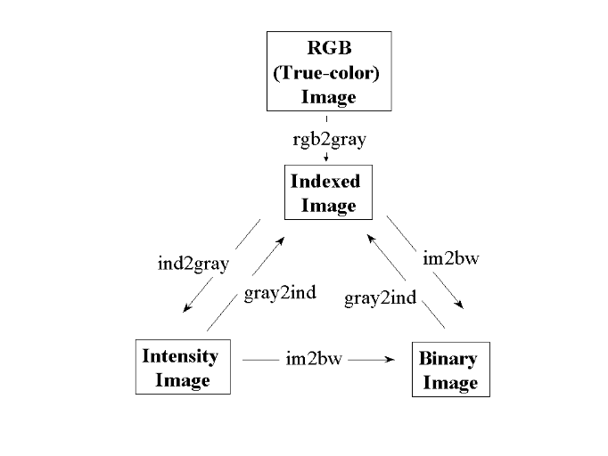
Figure 3.1: Conversion between different image
types.
3.2. EQUIPMENTS USED.
I n order to accomplish our project, we are used the
equipments such as digital computer in processing of the object(image) and
digital camera as the source of images. We can found more details of these
equipments in section 2.2 and section 2.3.
3.3. MATERIALS USED.
In conducting this research, we were used materials of images
like photos as samples.
The file formats of the used photos are:
JPEG means joint photograph expert graphics and BMP which means
bitmap format.
3.4. DETECTING AN OBJECT
USING IMAGE SEGMENTATION.
An object can be easily detected in an image if the object has
sufficient contrast from the background. We use edge detection and basic
morphology tools to detect a prostate cancer cell. To conduct this detection,
there are many steps to follow:
v Step 1: Read Image
v Step 2: Convert RGB to Gray
v Step 3: Detect Entire object
v Step 4: fill the gaps
v Step 5: Dilate the Image
v Step 6: Fill Interior Gaps
v Step 7: Remove Connected Objects on Border
v Step 8: Smooth the Object
STEP 1: READ IMAGE.
Read in 'filename.gpj', which is an image of a prostate cancer
filename.
I = imread('filename.jpg');
%filename is the name of the object to be detected and .jpg is
the file format of this image.
figure, imshow(I), title('original image'); % shows the
figure to be red.
STEP 2: CONVERT RGB TO GRAY
The image to be detected is the colour image, to detect it
correctly; we have to convert it into gray scale (intensity value) using the
command «rgb2gray».
rgb2gray(`filename.jpg');
newmap=rgb2gray(I);
figure, imshow(newmap), title(`gray image'); % shows the
converted figure.
STEP 3: DETECT ENTIRE OBJECT.
We will detect this object; another word for object detection
is segmentation. The object to be segmented differs greatly in contrast from
the background image. Changes in contrast can be detected by operators; that
calculate the gradient of an image. One way to calculate the gradient of an
image is the Sobel operator, which creates a binary mask using a user-specified
threshold value. We determine a threshold value using the graythresh function.
To create the binary gradient mask, we use the edge function.
BWs = edge (I, 'sobel', (graythresh(I) * .1)); % detects edges of
processed image.
% BWs means binary gradient mask
figure, imshow(BWs), title('binary gradient mask'); %shows the
binary gradient mask.
STEP 4: FILL GAPS
The binary gradient mask shows lines of high contrast in the
image. These lines do not quite delineate the outline of the object of
interest. Compared to the original image, you can see gaps in the lines
surrounding the object in the gradient mask. These linear gaps will disappear
if the Sobel image is dilated using linear structuring elements, which we can
create with the strel function.
se90 = strel ('line', 3, 90);
se0 = strel ('line', 3, 0);
STEP 5: DILATE THE IMAGE
The binary gradient mask is dilated using the vertical
structuring element followed by the horizontal structuring element. The
imdilate function dilates the image.
BWsdil = imdilate(BWs, [se90 se0]);
figure, imshow(BWsdil), title('dilated gradient mask');
STEP 6: FILL INTERIOR GAPS
The dilated gradient mask shows the outline of the cell quite
nicely, but there are still holes in the interior of the cell. To fill these
holes we use the imfill function.
BWdfill = imfill(BWsdil, 'holes');
figure, imshow(BWdfill), title('binary image with filled
holes');
STEP 7: REMOVE CONNECTED OBJECTS ON BORDER
(This step will be used when there are others object on the
border of the detected object). The object of interest has been successfully
segmented, but it is not the only object that has been found. Any objects that
are connected to the border of the image can be removed using the imclearborder
function. The connectivity in the imclearborder function was set to 4 to remove
diagonal connections.
BWnobord = imclearborder(BWdfill, 4);
STEP 8: SMOOTH THE OBJECT
Finally figure, imshow(BWnobord), title('cleared border
image');
, in order to make the segmented object look natural, we
smooth the object by eroding the image twice with a diamond-structuring
element. We create the diamond-structuring element using the strel function.
seD = strel('diamond',1);
BWfinal = imerode(BWnobord,seD);
BWfinal = imerode(BWfinal,seD);
figure, imshow(BWfinal), title('segmented image');
An alternate method for displaying the segmented object would
be to place an outline around the segmented object. The outline is created by
the bwperim function.
BWoutline = bwperim(BWfinal);
Segout = I;
Segout(BWoutline) = 255;
figure, imshow(Segout), title('outlined original image');
| 

