|
![]()
![]()
![]()
BAYESIAN PORTFOLIO SELECTION: An empirical Analysis of
the JSE-ALSI 2003-2010
M. Frankie MBUYAMBA
MCom Financial Economics (2010), University of Johannesburg,
(frankiem@uj.ac.za)
1. Abstract
Finance theory can be used to form informative prior beliefs
in financial decision making. This paper approaches portfolio selection in a
Mean-Variance, Mean-Conditional Variance and Black Litterman covariance and
Bayesian framework that incorporates a prior degree of belief in an asset
pricing model. Sample evidence on a period of 8 years and value and size
effects is evaluated from an asset-allocation perspective. Investor's belief in
the domestic CAPM must be very strong to justify the home bias observed in
their equity holdings. The same strong prior belief results in large and stable
optimal positions in this selection.
Keywords: Bayesian CAPM, Bayesian
portfolio selection, Black-Litterman(BL)
2. INTRODUCTION
Modem portfolio theory has providing a really framework for
portfolio optimization when investors who are risk-averse prefer investment
portfolios that are mean-variance efficient. Optimal portfolio selection
requires knowledge of each asset's expected return, variance, and covariance
with other asset returns. In practice, each asset's expected return, variance,
and covariance with other asset returns are unknown and must be estimated from
available historical or subjective information. We assume that the portfolio
manager has a goal of maximizing the expected return for a given level of risk.
We use monthly data comprise the performance of the benchmark; JSE-ALSI, to
capture the behaviour of weekly data in 400 observations of prices. We
construct our analysis by applying the mean conditional Value at Risk in order
to determine the weights of the portfolio and after that the paper is
implementing the work of Black and Litterman by using the variance-covariance
matrix so that we can provide an analysis of asset allocation and the weights
of choice of the optimal portfolio. Finally we look at the theory related to
the Black Litterman Bayesian CAPM where we use the benchmark, the risk free
rate and each of every stock so that we can have the weight value of the
portfolio to be mean-variance efficient to the market stock.
In our analysis we are looking to the Bayesian portfolio
selection because it's encountered the uncertainties problems of investors
while the Mean-Variance model ignores them. The fundamental of Bayesian
approach in portfolio selection is based on the notion of probability which is
defined by a degree of belief and makes possible to incorporate a belief about
the hypothesis which is valid to the probability that its alternative is valid.
One of the major matters with mean-variance models is the function between
variance-covariance/expected return inputs and the optimal portfolio weights is
highly nonlinear and can be very sensitive to the small changes in the views of
the manager1(*). The above
reasoning tells us that errors in covariance estimation are less damaging than
errors in covariance estimation which have less damage compare to the
estimation error in the expected return.
The paper is based in the first section on presenting the
paradigm of the portfolio optimization under uncertainty. The second section
will describe the models and methods of capturing the distributions of the
returns in three stages. The third section will be the presentation of the
empirical results on the ALSI and the height stocks since 1995 till now. The
last section is showing the implications of our results by stating the
relevance, implications and significance of the findings.
3. METHODOLOGY AND MODELLING
a) Mean-VaR Portfolio Selection
The expected return on the portfolio by minimizing the variance
of return will be like this:
Min 12XT?Xsubject to { XTi = 1 and XTu = up
(1)
We assume in the model that the market has n assets, the rate
of return of a single asset i is a random variable and the expected rate of
return for the asset is estimated through the observed return of the asset at
time t. Then ri =1Tt=1TRit (2)
The mean conditional VaR; Max {E (rp) - CVaRá
(rp); this is the alternative (or supplement) to VaR and it capture
the risk metric for continuous distributions.
For continuous distributions, CVaR, also known as the Mean
Excess Loss, Mean Shortfall, and Tail VaR, is the conditional expected loss
given that the loss exceeds VaR. That is, CVaR is given by
öá(x)= ?(1- á)?^2 ?_(f
(x,y)>æ(x,á)) f (x, y)p(y)dy,
(3)
The method to be used in this framework first is the
Mean-Variance that determines the weight of the portfolio and the mean VaR
weight in order to have the mean of return and the portfolio risk. The
following step is looking to the budget risk where we have the mean of the
portfolio return and the portfolio risk according to the Mean Conditional Value
at Risk (MCVaR).
b) Bayesian portfolio selection
The Bayesian portfolio selection is coming from conditional
probability distribution and it provides inferences about the distribution of
returns which is unknown by applying available signal or information.
The inference makes the probability statements about the generating process of
return.
Bayesian theorem is used to determine what one's probability
for the hypothesis should be, once the outcome D from the experiment is known.
The probability of the hypothesis once the outcome from the experiment is known
is called the posterior probability2(*).
p(èA) = P(A,?)p(A)=pA?p(?)p(A)
p(èA)?P(Aè)P(è) Posterior?Likelihood
x Prior (4) The prior is normally distributed and the
posterior probability is proportional to the likelihood of the observed data,
multiplied by the prior probability, and is given by Bayes' theorem. As the
investor with rational behavior will provide a predictive mean-variance
p(Rt+1At) (5) The equation (4) is called the posterior
distribution of future returns Let t denote the time, R the expected return and
A the historical return data observed.
To predict we observe A, and compute p(A) the predictive
distribution
P(A) = ?p(è)p(èA)dè
(6). The regression model will be Yi=Xiß+?i where
?i~Normal(0,ói) (7).
Bayesian regression model of joint distribution of Y and X
P(X,Y)= P(XØ)P(YX,â,s2) (8) Where Ø is
a priori or a set of information independent of (â,ó).
At this stage we will compare two methods of Black Litterman
where the first one will consist on the covariance through the BLCOP in order
to get the weight and the risk of the portfolio by using the historical returns
and the other stage will be based on the Bayesian CAPM which generates the
alpha and beta coefficient of each stock by using the Markov Chain Monte Carlo
package in R software (MCMC pack), we applying the excess return observed and
the alpha in addition with the beta which forms the product with the excess
market estimate in order to obtain the excess return of each stock estimate and
after that we use the covariance of this dataset according to BLCOP where we
have the weight and risk of the portfolio.
4. EMPIRICAL RESULTS
Fig.1
![]()
Fig.1
|
Portf Mean
|
Portf Risk
|
VaR
|
CVaR
|
|
M-V
|
0.0024
|
0.0171
|
0.0242
|
0.0372
|
|
MCVaR
|
0.00208
|
0.02274
|
0.0285
|
0.043
|
|
BL Cov
|
0.0032
|
0.0214
|
0.0000
|
0.0000
|
|
BL CAPM
|
0.0034
|
0.0221
|
|
|
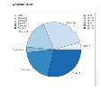
In this empirical section we consider the weekly return data
on the JSE-ALSI from early February 2003 till late September 2010. The market
capitalization weights on the efficient portfolio are dominant of 24.9% on the
USD/ZAR exchange rate following by Chemical Index and there is no weight
allocated to Life insurance Index. The mean conditional variance is giving the
following figures through the risk budgets; the highest shares are in chemical,
technology and beverage by respectively 22.7%, 22.6% and 20.1%. The life
insurance stills the only stock which doesn't have any allocation.
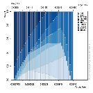
The fig.1 tells us that at a lowest risk with almost all the
weight will be allocated to USDZAR and some negative return on the USDZAR and
Technology Index. It's telling us also that at optimal point we have to
combine an important weight of the USDZAR with a target return of 0.000662 and
risk profile of 0.0111, following by Technology Index and almost a close weight
between the Bank Index and the Chemical. The highest level of risk will be
achieved with a target return of 0.0049 and Telecom will have the entire
maximum weight allocated.
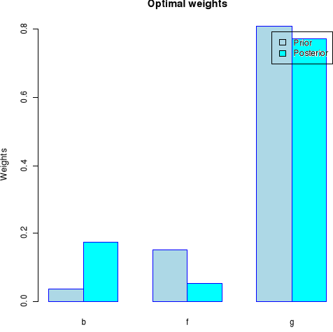
The prior of the beverage index is very low to his posterior
while telecom has a high prior than the posterior. The highest weight is found
on the technology index where the prior and the posterior are almost closer to
0.8.
On fig.2 we have a highest portfolio mean on a Bayesian CAPM
which is the higher expected return and the lowest risk of the portfolio is
assigned to the Mean-Variance method. The highest expected value which can be
loosed and the highest expected value plus all negative losses is given by the
mean conditional value at risk method.
5. CONCLUSION
Traditional mean-variance portfolio optimization assumes that
it is extremely difficult to estimate expected returns precisely. In practice,
portfolios that ignore estimation error have very poor properties: the
portfolio weights have extreme values that fluctuate dramatically over time and
deliver very low Sharpe ratios over time. The Bayesian approach allows a
Bayesian investor to include a certain degree of belief in a portfolio
selection model. In this paper, we have shown how to allow
for the possibility of multiple priors about the estimated expected returns and
the underlying market return model. And, in addition to the standard
optimization of the mean-variance objective function over the choice of
weights, one also will provide the lowest value at risk and the conditional
value at risk. This study uses theoretically motivated prior and posterior
information about expected returns in portfolio selection. From an estimation
perspective, the focus on expected returns could be helpful since it is well
known that means are in general estimated with much less precision than
covariance. Nevertheless, using prior information to impose some structure on
the Black Litterman covariance matrix could potentially also be beneficial,
especially for a large number of stocks.
Reference
1. Polson, N. G., and Tew, B. V., 2000. Bayesian
portfolio selection: An empirical analysis of the S&P 500 index
1970-1996. Journal of Business & Economic Statistics,
18(2)
2. J.M MWAMBA, Slides of Bayesian asset pricing,
MCom Financial Economics, 2010
6. Appendix
VaR.5% : -0.02851397 CVaR.5% : -0.04303770
Title:
MV Efficient Portfolio
Portfolio Weights:
Alsi Bank Beverage Chemical Equity.Inv Life.Insur
Telecom
0.0000 0.0854 0.1421 0.2242 0.0747 0.0000
0.0958
Technol USDZAR Risk.free
0.1244 0.2489 0.0044
Covariance Risk Budgets:
Alsi Bank Beverage Chemical Equity.Inv Life.Insur
Telecom
0.0000 0.1034 0.2012 0.2256 0.0814 0.0000
0.1432
Technol USDZAR Risk.free
0.2270 0.0185 -0.0003
Target Return and Risks:
mean mu Cov Sigma CVaR VaR
0.0024 0.0024 0.0171 0.0171 0.0372 0.0242
![]()
Iterations = 1001:11000
Thinning interval = 1
Number of chains = 1
Sample size per chain = 10000
1. Empirical mean and standard deviation for each variable,
plus standard error of the mean:
Mean SD Naive SE Time-series
SE
(Intercept) -0.0001138 8.713e-04 8.713e-06
1.073e-05
Dataset$Bank 0.1434273 3.481e-02 3.481e-04
2.628e-04
Dataset$Beverage 0.2692399 3.065e-02 3.065e-04
2.718e-04
Dataset$Chemical 0.1113228 3.898e-02 3.898e-04
3.467e-04
Dataset$Equity.Inv 0.0349513 3.327e-02 3.327e-04
3.460e-04
Dataset$Life.Insur 0.1670380 3.429e-02 3.429e-04
3.237e-04
Dataset$Telecom 0.1217420 2.772e-02 2.772e-04
2.699e-04
Dataset$Technol 0.1121895 2.673e-02 2.673e-04
2.366e-04
Dataset$USDZAR -0.0245311 3.799e-02 3.799e-04
3.799e-04
sigma2 0.0003003 2.175e-05 2.175e-07
2.134e-07
2. Quantiles for each variable:
2.5% 25% 50% 75%
97.5%
(Intercept) -0.0018314 -0.0007030 -0.0001028 0.0004741
0.0015800
Dataset$Bank 0.0758993 0.1192552 0.1433875 0.1667630
0.2121726
Dataset$Beverage 0.2088588 0.2486275 0.2690060 0.2898102
0.3288659
Dataset$Chemical 0.0353141 0.0851677 0.1112476 0.1371965
0.1893481
Dataset$Equity.Inv -0.0310190 0.0126328 0.0350995 0.0573648
0.1001137
Dataset$Life.Insur 0.0991277 0.1438379 0.1670621 0.1899787
0.2345747
Dataset$Telecom 0.0672014 0.1030527 0.1216117 0.1406669
0.1759571
Dataset$Technol 0.0593993 0.0945787 0.1124306 0.1299468
0.1643140
Dataset$USDZAR -0.0993244 -0.0497875 -0.0244516 0.0011008
0.0491126
sigma2 0.0002603 0.0002851 0.0002993 0.0003141
0.0003461
$priorPfolioWeights
a b c d e f
g
0.00000000 0.03770282 0.00000000 0.00000000 0.00000000 0.15294225
0.80935492
h
0.00000000
$postPfolioWeights
a b c d e f
g h
0.00000000 0.17475666 0.00000000 0.00000000 0.00000000 0.05346057
0.77178277
0.00000000
![]()
Title:
MV Tangency Portfolio
Estimator: .priorEstim
Solver: solveRquadprog
Optimize: minRisk
Constraints: LongOnly
Portfolio Weights:
a b c d e f g h
0.0417 0.2299 0.2235 0.0374 0.0000 0.1561 0.1818 0.1297
Covariance Risk Budgets:
a b c d e f g h
Target Return and Risks:
mean mu Cov Sigma CVaR VaR
0.0000 0.0030 0.0213 0.0000 0.0000
Description:
Tue Sep 28 15:35:54 2010 by user: General
$posteriorOptimPortfolio
Title:
MV Tangency Portfolio
Estimator: .posteriorEstim
Solver: solveRquadprog
Optimize: minRisk
Constraints: LongOnly
Portfolio Weights:
a b c d e f g h
0.0064 0.2508 0.2846 0.0000 0.0000 0.1357 0.1875 0.1350
Covariance Risk Budgets:
a b c d e f g h
Target Return and Risks:
mean mu Cov Sigma CVaR VaR
0.0000 0.0032 0.0214 0.0000 0.0000
Description:
Tue Sep 28 15:35:54 2010 by user: General
attr(,"class")
[1] "BLOptimPortfolios"
Iterations = 1001:11000
Thinning interval = 1
Number of chains = 1
Sample size per chain = 10000
1. Empirical mean and standard deviation for each variable,
plus standard error of the mean:
Mean SD Naive SE Time-series SE
(Intercept) 0.0009522 9.041e-04 9.041e-06 1.113e-05
Dataset$ebank 0.1398387 3.472e-02 3.472e-04 2.861e-04
Dataset$ebev 0.2688045 3.071e-02 3.071e-04 2.712e-04
Dataset$echem 0.1319496 3.712e-02 3.712e-04 3.282e-04
Dataset$eequit 0.0540071 3.231e-02 3.231e-04 3.318e-04
Dataset$elife 0.1775072 3.386e-02 3.386e-04 3.226e-04
Dataset$etelec 0.1266767 2.786e-02 2.786e-04 2.673e-04
Dataset$etech 0.1179304 2.654e-02 2.654e-04 2.457e-04
Dataset$eusazar -0.0094296 3.607e-02 3.607e-04 3.740e-04
sigma2 0.0003012 2.182e-05 2.182e-07 2.140e-07
2. Quantiles for each variable:
2.5% 25% 50% 75%
97.5%
(Intercept) -0.0008301 0.0003408 0.0009637 0.0015623
0.0027097
Dataset$ebank 0.0720157 0.1161651 0.1402517 0.1631226
0.2073024
Dataset$ebev 0.2085894 0.2482177 0.2686163 0.2893781
0.3291133
Dataset$echem 0.0599178 0.1070750 0.1317707 0.1565901
0.2057048
Dataset$eequit -0.0100727 0.0322763 0.0539325 0.0757838
0.1172233
Dataset$elife 0.1106212 0.1548548 0.1774808 0.2002120
0.2440648
Dataset$etelec 0.0719587 0.1081133 0.1265930 0.1455601
0.1808797
Dataset$etech 0.0657202 0.1002334 0.1182699 0.1358541
0.1696935
Dataset$eusazar -0.0808365 -0.0333380 -0.0095017 0.0147699
0.0617244
sigma2 0.0002611 0.0002860 0.0003002 0.0003151
0.0003471
* 1 Further reading of Polson
and Tew
* 2 Slides of Bayesian asset
pricing
| 
