ANNEXE
ANNEXE 1 :
a) LES DONNEES UTILISEES
|
OBS
|
PIBK_A
|
SKP_A
|
SKH_A
|
PAO_A
|
|
1990
|
184,10
|
18,27
|
2,23
|
1,09
|
|
1991
|
199,00
|
18,34
|
2,32
|
1,13
|
|
1992
|
200,30
|
18,77
|
2,41
|
1,17
|
|
1993
|
220,60
|
18,85
|
2,62
|
1,18
|
|
1994
|
227,80
|
18,86
|
2,82
|
1,19
|
|
1995
|
241,00
|
19,06
|
3,02
|
1,20
|
|
1996
|
254,50
|
19,21
|
3,21
|
1,21
|
|
1997
|
270,00
|
19,23
|
3,40
|
1,22
|
|
1998
|
284,10
|
19,27
|
3,57
|
1,23
|
|
1999
|
301,10
|
19,27
|
3,74
|
1,24
|
|
2000
|
314,70
|
19,42
|
3,90
|
1,25
|
|
2001
|
334,80
|
19,50
|
4,04
|
1,26
|
|
2002
|
343,00
|
19,72
|
4,16
|
1,27
|
|
2003
|
350,70
|
19,56
|
4,28
|
1,29
|
|
2004
|
372,80
|
19,63
|
4,38
|
1,30
|
|
2005
|
369,70
|
19,78
|
4,49
|
1,31
|
|
2006
|
390,20
|
27,61
|
4,58
|
1,32
|
|
2007
|
406,70
|
36,71
|
4,67
|
1,33
|
|
2008
|
421,20
|
39,63
|
4,76
|
1,34
|
|
2009
|
431,75
|
30,69
|
4,84
|
1,35
|
PIBK_A : Produit Intérieur Brut à
prix constant du secteur primaire en milliards de FCFA (Source : comptes
nationaux INSAE)
SKP_A : Stock de Capital Physique du secteur
Primaire en milliards de FCFA (Source : Calcul auteur sur données du
MAPES)
SKH_A : Stock de Capital humain dans
l'agriculture en millions d'années d'instruction (Source : calcul auteur
sur données des RGPH1, RGPH2 RGPH3)
PAO_A : Population Active Occupée dans
l'Agriculture en millions d'emplois effectifs (Source : calcul auteur sur
données des RGPH1, RGPH2 et RGPH3)
b) Nom et libellés des variables
utilisées
|
Nom des variables
|
Libellés des variables
|
|
PIBK_A
|
Produit Intérieur Brut agricole à prix constant
|
|
SKP_A
|
Stock de Capital Physique dans l'agriculture
|
|
SKH_A
|
Stock de Capital Humain dans l'Agriculture
|
|
PAO_A
|
Population Active Occupée dans l'agriculture
|
|
PGF
|
Productivité Global des Facteurs
|
|
L+ Nom de variables
|
Logarithme naturel de la variable
|
|
G+ Nom de Variable
|
Taux de croissance de la variable
|
|
Nom de Variables + S ou Nom de Variables + FOR
|
Variables estimées ou variables simulées
|

ANNEXE 2 : TESTS DE RACINE UNITAIRE SUR LES SERIES a)
Tests de racine unitaire sur log (skh_a)
Null Hypothesis: D(LOG(SKH_A)) has a unit root Exogenous:
Constant, Linear Trend
Lag Length: 1 (Automatic based on SIC, MAXLAG=1)
t-Statistic Prob.*
Augmented Dickey-Fuller test statistic -8.889699
0.0000
Test critical values: 1% level -4.616209
5% level -3.710482
10% level -3.297799
*MacKinnon (1996) one-sided p-values.
Warning: Probabilities and critical values calculated for 20
observations and may not be accurate for a sample size of 17
Augmented Dickey-Fuller Test Equation Dependent Variable:
D(LOG(SKH_A),2) Method: Least Squares
Date: 09/28/10 Time: 21:58
Sample (adjusted): 1993 2009
Included observations: 17 after adjustments
|
Variable
|
Coefficient
|
Std. Error t-Statistic
|
Prob.
|
|
D(LOG(SKH_A(-1)))
|
-1.175281
|
0.132207 -8.889699
|
0.0000
|
|
D(LOG(SKH_A(-1)),2)
|
0.174435
|
0.110055 1.584981
|
0.1370
|
|
C
|
0.099417
|
0.010867 9.148629
|
0.0000
|
|
@TREND(1990)
|
-0.004612
|
0.000507 -9.103692
|
0.0000
|
|
R-squared
|
0.873369
|
Mean dependent var
|
-0.001117
|
|
Adjusted R-squared
|
0.844146
|
S.D. dependent var
|
0.012977
|
|
S.E. of regression
|
0.005123
|
Akaike info criterion
|
-7.507811
|
|
Sumsquaredresid
|
0.000341
|
Schwarz criterion
|
-7.311761
|
|
Log likelihood
|
67.81639
|
F-statistic
|
29.88681
|
|
Durbin-Watson stat
|
0.387358
|
Prob(F-statistic)
|
0.000004
|
b) Test de racine unitaire sur log (SKP_A)
Null Hypothesis: D(LOG(SKP_A)) has a unit root Exogenous: None
Lag Length: 0 (Automatic based on SIC, MAXLAG=0)
t-Statistic Prob.*
Augmented Dickey-Fuller test statistic -1.978645
0.0483
Test critical values: 1% level -2.699769
5% level -1.961409
10% level -1.606610
*MacKinnon (1996) one-sided p-values.
Warning: Probabilities and critical values calculated for 20
observations and may not be accurate for a sample size of 18
Augmented Dickey-Fuller Test Equation Dependent Variable:
D(LOG(SKP_A),2) Method: Least Squares
Date: 09/28/10 Time: 22:06
Sample (adjusted): 1992 2009
Included observations: 18 after adjustments
|
Variable
|
Coefficient
|
Std. Error t-Statistic
|
Prob.
|
|
D(LOG(SKP_A(-1)))
|
-0.497702
|
0.251537 -1.978645
|
0.0643
|
|
R-squared
|
0.175506
|
Meandependent var
|
-0.014407
|
|
Adjusted R-squared
|
0.175506
|
S.D. dependent var
|
0.123660
|
|
S.E. of regression
|
0.112286
|
Akaike info criterion
|
-1.481589
|
|
Sumsquaredresid
|
0.214337
|
Schwarz criterion
|
-1.432123
|
|
Log likelihood
|
14.33430
|
Durbin-Watson stat
|
1.107626
|

c) Test de racine unitaire sur log (PIBK_A)
Null Hypothesis: D(LOG(PIBK_A)) has a unit root Exogenous:
Constant, Linear Trend
Lag Length: 0 (Automatic based on SIC, MAXLAG=0)
t-Statistic Prob.*
Augmented Dickey-Fuller test statistic -8.720221
0.0000
Test critical values: 1% level -4.571559
5% level -3.690814
10% level -3.286909
*MacKinnon (1996) one-sided p-values.
Warning: Probabilities and critical values calculated for 20
observations and may not be accurate for a sample size of 18
Augmented Dickey-Fuller Test Equation Dependent Variable:
D(LOG(PIBK_A),2) Method: Least Squares
Date: 09/28/10 Time: 22:09
Sample (adjusted): 1992 2009
Included observations: 18 after adjustments
|
Variable
|
Coefficient
|
Std. Error t-Statistic
|
Prob.
|
|
D(LOG(PIBK_A(-1)))
|
-1.650782
|
0.189305 -8.720221
|
0.0000
|
|
C
|
0.097876
|
0.015334 6.382732
|
0.0000
|
|
@TREND(1990)
|
-0.002374
|
0.000882 -2.690150
|
0.0168
|
|
R-squared
|
0.835408
|
Meandependent var
|
-0.002950
|
|
Adjusted R-squared
|
0.813462
|
S.D. dependent var
|
0.042271
|
|
S.E. of regression
|
0.018257
|
Akaike info criterion
|
-5.017561
|
|
Sumsquaredresid
|
0.005000
|
Schwarz criterion
|
-4.869166
|
|
Log likelihood
|
48.15805
|
F-statistic
|
38.06714
|
|
Durbin-Watson stat
|
1.789591
|
Prob(F-statistic)
|
0.000001
|

d) Tests de racine unitaire sur log (PAO_A)
Null Hypothesis: D(LOG(PAO_A)) has a unit root Exogenous:
Constant
Lag Length: 1 (Automatic based on SIC, MAXLAG=1)
t-Statistic Prob.*
Augmented Dickey-Fuller test statistic -69.82077
0.0000
Test critical values: 1% level -3.886751
5% level -3.052169
10% level -2.666593
*MacKinnon (1996) one-sided p-values.
Warning: Probabilities and critical values calculated for 20
observations and may not be accurate for a sample size of 17
Augmented Dickey-Fuller Test Equation Dependent Variable:
D(LOG(PAO_A),2) Method: Least Squares
Date: 09/28/10 Time: 22:16
Sample (adjusted): 1993 2009
Included observations: 17 after adjustments
|
Variable
|
Coefficient
|
Std. Error t-Statistic
|
Prob.
|
|
D(LOG(PAO_A(-1)))
|
-0.968573
|
0.013872 -69.82077
|
0.0000
|
|
D(LOG(PAO_A(-1)),2)
|
-0.026147
|
0.014326 -1.825191
|
0.0894
|
|
C
|
0.008293
|
0.000161 51.53149
|
0.0000
|
|
R-squared
|
0.997137
|
Mean dependent var
|
-0.001425
|
|
Adjusted R-squared
|
0.996728
|
S.D. dependent var
|
0.005567
|
|
S.E. of regression
|
0.000318
|
Akaike info criterion
|
-13.10748
|
|
Sumsquaredresid
|
1.42E-06
|
Schwarz criterion
|
-12.96044
|
|
Log likelihood
|
114.4136
|
F-statistic
|
2438.294
|
|
Durbin-Watson stat
|
0.242785
|
Prob(F-statistic)
|
0.000000
|
ANNEXE 3 : ESTIMATION DES FONCTIONS DE
PRODUCTION
a) modèle de Solow à deux facteurs (capital et
travail)
Dependent Variable: LOG(PIBK_A)
Method: Least Squares
Date: 09/29/10 Time: 01:43
Sample(adjusted): 1991 2009
Included observations: 19 after adjusting endpoints
Convergence achievedafter 5 iterations
LOG(PIBK_A)=C(1)+C(2)*LOG(SKP_A)+(1-C(2))*LOG(PAO_A)
+[AR(1)=C(3)]+C(4)*D92+C(5)*D04
Coefficient Std. Error t-Statistic Prob.
C(1) 12.98178 0.615826 21.08026 0.0000
C(2) 0.040694 0.026417 1.540405 0.1458
C(4) -0.057142 0.009226 -6.193621 0.0000
C(5) 0.034323 0.009221 3.722272 0.0023
C(3) 0.967352 0.015784 61.28689 0.0000
R-squared 0.997989 Mean dependent var 26.43797
Adjusted R-squared 0.997414 S.D. dependent var 0.252289
S.E. of regression 0.012828 Akaike info criterion -5.653378
Sumsquaredresid 0.002304 Schwarz criterion -5.404841
Log likelihood 58.70709 F-statistic 1736.957
Durbin-Watson stat 1.374233 Prob(F-statistic) 0.000000
Inverted AR Roots .97
b) fonction de production de long terme
Dependent Variable: LOG(PIBK_A)
Method: Least Squares
Date: 09/29/10 Time: 00:52
Sample(adjusted): 1991 2009
Included observations: 19 after adjusting endpoints
Convergence achieved after 9 iterations
LOG(PIBK_A)=C(1)+C(2)*LOG(SKP_A)+C(3)*LOG(SKH_A)+(1-C(2)
-C(3))*LOG(PAO_A)+[AR(1)=C(4)]+C(5)*D91+C(6)*D04+C(7)*D01
+C(8)*D93
Coefficient Std. Error t-Statistic Prob.
C(1) 10.89271 0.299194 36.40683 0.0000
C(2) 0.045766 0.015026 3.045700 0.0111
C(3) 0.709734 0.107967 6.573621 0.0000
C(5) 0.034610 0.005269 6.568284 0.0000
C(6) 0.034452 0.005266 6.542007 0.0000
C(7) 0.017747 0.005270 3.367613 0.0063
C(8) 0.028672 0.005294 5.415967 0.0002
C(4) 1.042529 0.042849 24.33034 0.0000
R-squared 0.999445 Meandependent var 26.43797
Adjusted R-squared 0.999091 S.D. dependent var 0.252289
S.E. of regression 0.007606 Akaike info criterion -6.624276
Sumsquaredresid 0.000636 Schwarz criterion -6.226617
Log likelihood 70.93062 F-statistic 2827.809
Durbin-Watson stat 1.583911 Prob(F-statistic) 0.000000
Inverted AR Roots 1.04
Estimated AR process is nonstationary
c) Test de racine unitaire sur les résidus issus
du modèle de long terme (RESIDUSLT=résidus issus du modèle
de long terme)
Null Hypothesis: RESIDUSLT has a unit root
Exogenous: None
Lag Length: 0 (Automatic based on SIC, MAXLAG=3)
t-Statistic Prob.*
Augmented Dickey-Fuller test statistic -3.324892
0.0023
Test critical values: 1% level -2.699769
5% level -1.961409
10% level -1.606610
*MacKinnon (1996) one-sided p-values.
Warning: Probabilities and critical values calculated for 20
observations and may not be accurate for a sample size of 18
Augmented Dickey-Fuller Test Equation Dependent Variable:
D(RESIDUSLT) Method: Least Squares
Date: 09/28/10 Time: 22:59
Sample (adjusted): 1992 2009
Included observations: 18 after adjustments
|
Variable
|
Coefficient
|
Std. Error t-Statistic
|
Prob.
|
|
RESIDUSLT(-1)
|
-0.809578
|
0.243490 -3.324892
|
0.0040
|
|
R-squared
|
0.392209
|
Mean dependent var
|
0.000411
|
|
Adjusted R-squared
|
0.392209
|
S.D. dependent var
|
0.007688
|
|
S.E. of regression
|
0.005994
|
Akaike info criterion
|
-7.342212
|
|
Sumsquaredresid
|
0.000611
|
Schwarz criterion
|
-7.292747
|
|
Log likelihood
|
67.07991
|
Durbin-Watson stat
|
2.012627
|
d) Fonction de production de court terme
Dependent Variable: D(LOG(PIBK_A))
Method: Least Squares
Date: 09/29/10 Time: 00:55
Sample(adjusted): 1992 2009
Included observations: 18 after adjusting endpoints
D(LOG(PIBK_A))=C(1)+C(2)*D(LOG(SKP_A))+C(3)*D(LOG(SKH_A))
+(1-C(2)-C(3))*D(LOG(PAO_A))+C(4)*RESIDUSLT(-1)+C(5)*D94
+C(6)*D05+C(7)*D92+C(8)*D95+C(9)*D96+C(10)*D01+C(11)*D02
+C(12)*D03
|
Coefficient Std. Error t-Statistic
|
Prob.
|
C(1)
|
0.018414 0.003540 5.201111
|
0.0020
|
C(2)
|
0.033181 0.012612 2.630866
|
0.0390
|
C(3)
|
0.837787 0.097161 8.622634
|
0.0001
|
C(4)
|
-1.096157 0.280529 -3.907465
|
0.0079
|
C(5)
|
-0.053198 0.007363 -7.224597
|
0.0004
|
C(6)
|
-0.055084 0.006829 -8.065924
|
0.0002
|
C(7)
|
-0.049174 0.006900 -7.126597
|
0.0004
|
C(8)
|
-0.022990 0.007047 -3.262484
|
0.0172
|
C(9)
|
-0.019902 0.006845 -2.907747
|
0.0271
|
C(10)
|
0.014038 0.006409 2.190390
|
0.0710
|
C(11)
|
-0.016679 0.006553 -2.545354
|
0.0438
|
C(12)
|
|
-0.015372 0.006625 -2.320474
|
0.0594
|
|
|
R-squared
|
0.977421 Mean dependent var
|
0.043030
|
|
Adjusted R-squared
|
0.936026 S.D. dependent var
|
0.024018
|
|
S.E. of regression
|
0.006075 Akaike info criterion
|
-7.134564
|
|
Sumsquaredresid
|
0.000221 Schwarz criterion
|
-6.540983
|
|
Log likelihood
|
76.21108 F-statistic
|
23.61222
|
|
Durbin-Watson stat
|
1.937422 Prob(F-statistic)
|
0.000476
|
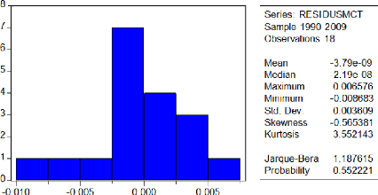

e) Test de normalité des résidus du
MCE

f) AUTOCCORELOGRAMME DES RESIDUS DU MODELE DYNAMIQUE DE
COURT TERME (test de bruit blanc)
Date: 09/29/10 Time: 18:05 Sample: 1990 2009
Included observations: 17
|
Autocorrelation
|
Partial Correlation
|
|
AC
|
PAC
|
Q-Stat
|
Prob
|
|
. **| . |
|
. **| . |
|
1
|
-0.278
|
-0.278
|
1.5561
|
0.212
|
|
. **| . |
|
.***| . |
|
2
|
-0.266
|
-0.372
|
3.0793
|
0.214
|
|
. *| . |
|
.***| . |
|
3
|
-0.073
|
-0.349
|
3.2034
|
0.361
|
|
. | . |
|
. **| . |
|
4
|
0.054
|
-0.307
|
3.2769
|
0.513
|
|
. |* . |
|
. **| . |
|
5
|
0.081
|
-0.243
|
3.4529
|
0.631
|
|
. | . |
|
. *| . |
|
6
|
0.035
|
-0.175
|
3.4888
|
0.745
|
|
. | . |
|
. | . |
|
7
|
0.059
|
0.014
|
3.6016
|
0.824
|
|
. | . |
|
. |* . |
|
8
|
-0.039
|
0.109
|
3.6567
|
0.887
|
|
. | . |
|
. |** . |
|
9
|
0.000
|
0.268
|
3.6567
|
0.933
|
|
. | . |
|
. |***. |
|
10
|
0.000
|
0.391
|
3.6567
|
0.962
|
g) Test d'homoscédasticité des erreurs
issues du MCE
ARCH Test:
F-statistic 0.420316 Probability 0.838464
Obs*R-squared 7.707749 Probability 0.462526
Test Equation:
Dependent Variable: RESID^2
Method: Least Squares
Date: 09/29/10 Time: 22:34
Sample(adjusted): 2000 2009
Included observations: 10 after adjusting endpoints
Variable Coefficient Std. Error t-Statistic Prob.
C 3.67E-05 4.14E-05 0.886533 0.5382
RESID^2(-1) -0.433900 0.903671 -0.480152 0.7150
RESID^2(-2) -0.501441 0.862769 -0.581200 0.6648
RESID^2(-3) -0.290359 0.490098 -0.592450 0.6595
RESID^2(-4) -0.151288 0.474166 -0.319061 0.8034
RESID^2(-5) -0.326557 0.436317 -0.748441 0.5910
RESID^2(-6) -0.355151 0.486007 -0.730752 0.5982
RESID^2(-7) 0.191870 0.494793 0.387778 0.7645
RESID^2(-8) -0.177400 0.521098 -0.340435 0.7911
R-squared 0.770775 Mean dependent var 1.11E-05
Adjusted R-squared -1.063026 S.D. dependent var 1.59E-05
S.E. of regression 2.28E-05 Akaike info criterion -19.04260
Sumsquaredresid 5.20E-10 Schwarz criterion -18.77027
Log likelihood 104.2130 F-statistic 0.420316
Durbin-Watson stat 2.689257 Prob(F-statistic) 0.838464
h) Résidus récursives
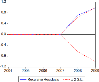
| 

