ANNEXES
45
Code Matlab du système
46
elseif P_pv < P_load && P_battery <= 0 % Si la
batterie est vide, on utilise le groupe électrogène P_supply =
P_pv + P_gen_max; % Groupe électrogène de secours
end
% Enregistrer les résultats après
amélioration P_pv_after = [P_pv_after, P_pv];
P_battery_after = [P_battery_after, P_battery]; P_supply_after =
[P_supply_after, P_supply];
end
% Création des graphiques pour comparer avant et
après amélioration figure;
% Graphique de la production photovoltaïque
subplot(3,1,1);
plot(P_pv_before, 'r', 'DisplayName', 'Production PV avant');
hold on;
plot(P_pv_after, 'g', 'DisplayName', 'Production PV
après');
title('Production Photovoltaïque');
legend;
xlabel('Temps (unités)');
ylabel('Puissance (kW)');
grid on;
% Graphique de l'énergie stockée dans la
batterie
subplot(3,1,2);
plot(P_battery_before, 'r', 'DisplayName', 'Batterie avant');
hold on;
plot(P_battery_after, 'g', 'DisplayName', 'Batterie
après');
title('Énergie de la Batterie');
legend;
xlabel('Temps (unités)');
ylabel('Énergie (kWh)');
grid on;
% Graphique de la puissance fournie au réseau
subplot(3,1,3);
plot(P_supply_before, 'r', 'DisplayName', 'Puissance fournie
avant');
hold on;
plot(P_supply_after, 'g', 'DisplayName', 'Puissance fournie
après');
title('Puissance Fournie au Réseau');
legend;
xlabel('Temps (unités)');
ylabel('Puissance (kW)');
grid on;
70
80
9 10
Puissance Tou mie aval!
Puis-sam. fournie apre
Production Photovoltaïque
P mdontian Pt+ auant
P modu1)ion YV apfès
! Ir
.1 "j!?
80 9O 100
1;543 1;11
Ili
I f ~I
0
4 10 20 30 40 50 60
Temps (unités)
Puissance Fournie au Biseau
10 20 30 40 50 60 79
Temps (unités) Énergie de la
Batterie
10 20 30 40 50 60 70 80 90 100
Temps (unItés)
% Export des résultats dans un fichier Excel
T = table(P_pv_before', P_battery_before', P_supply_before',
...
47
P_pv_after', P_battery_after', P_supply_after', ...
'VariableNames', {'PV_Avant', 'Batterie_Avant',
'Fourniture_Avant', ... 'PV_Apres', 'Batterie_Apres', 'Fourniture_Apres'});
writetable(T, 'resultats_simulation_micro_reseau.xlsx');
Enregistrement d'un graphique en GIF
filename = 'simulation_comparaison.gif';
for i = 1:length(P_pv_before)
Créer le graphique
figure;
plot(P_pv_before(1:i), 'r', 'DisplayName', 'Production PV
avant');
hold on;
plot(P_pv_after(1:i), 'g', 'DisplayName', 'Production PV
après');
plot(P_battery_before(1:i), 'b', 'DisplayName', 'Batterie
avant');
plot(P_battery_after(1:i), 'c', 'DisplayName', 'Batterie
après');
plot(P_supply_before(l:i), 'm', 'DisplayName', 'Puissance fournie
avant');
plot(P_supply_after(1:i), 'k', 'DisplayName', 'Puissance fournie
après');
title('Comparaison avant et après
amélioration');
legend;
xlabel('Temps (unités)');
ylabel('Puissance / Énergie (kW / kWh)');
grid on;
Capture du frame pour GIF frame = getframe(gcf); im =
frame2im(frame);
[A, map] = rgb2ind(im, 256);
if i == 1
imwrite(A, map, filename, 'gif', 'LoopCount', inf, 'DelayTime',
0.1);
else
imwrite(A, map, filename, 'gif', 'WriteMode', 'append',
'DelayTime', 0.1);
end
end
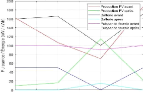
Comparaison avant et après
amélioration
Production PV avant Production PV apri=s Batterie avant
Batterie aprës Puissance fournie avant Puissance fournie
aprës
18,0
160
140
120
100
'W so

60
20
0.2 0.4 0.6 0.8 1 1.2 1.4 1.6 1.8 2
Temps (unités)
48
Sao 16a 140 120 100
· W Ba N
60
m
LL 40
20
n
Comparaison avant et après
amélioration
Production PV avant Production PV après Batterie avant
Batterie après Puissance fournie avant Puissance fournie
après
L

1.1 1.2 1.3 1.4 1.5 1.6 1.7 1.8 1.9 2
Temps (unités)
tan
160
140
120
100 7,1
· w 80 â)
60
En
-?
a 40
20
Comparaison avant et après
amélioration
Production PV avant Production PV après Batterie
avant
Batterie après Puissance fournie avant Puissance fournie
après
t2 1A 1.6 13 2 22 2.4 2.6 2.8 3
Temps (unités)
Comparaison avant et après
amélioration
LL
40
20
200
180
160
140
120
c 100
· W
Production PV avant Production PV après Batterie avant
Batterie après Puissance fournie avant Puissance fournie
après
3.5 4
1.5 2 2-5 3
Temps (unités)
49
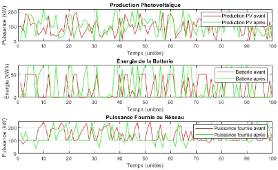
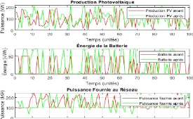
Figure 6 : les résultats de simulation : Avant et
après amélioration
Interprétation des résultats de
simulation : Avant et après amélioration
L'image ci-dessus présente trois sous-graphes comparant
les performances du micro-réseau de Tshumbe avant et après
l'implémentation des solutions d'amélioration proposées,
notamment l'intégration de compteurs intelligents, l'optimisation du
stockage d'énergie et l'amélioration de la gestion de la
production photovoltaïque. Chaque sous-graphe illustre l'évolution
de différentes variables clés du système, permettant de
visualiser l'impact des améliorations sur la production
d'énergie, le stockage et la fourniture au réseau.
|