1.
TEST DE STATIONNARITE SUR LES VARIABLES
Tableau n° 15 : Stationarisation en
différence première du LCR
|
Null Hypothesis: D(LCRE) has a unit root
|
|
|
Exogenous: None
|
|
|
|
LagLength: 0 (Fixed)
|
|
|
|
|
|
|
|
|
|
|
|
|
|
|
|
t-Statistic
|
Prob.*
|
|
|
|
|
|
|
|
|
|
|
|
Augmented Dickey-Fuller test statistic
|
-4.137609
|
0.0001
|
|
Test critical values:
|
1% level
|
|
-2.621185
|
|
|
5% level
|
|
-1.948886
|
|
|
10% level
|
|
-1.611932
|
|
|
|
|
|
|
|
|
|
|
|
|
*MacKinnon (1996) one-sided p-values.
|
|
|
|
|
|
|
|
|
|
|
|
|
Augmented Dickey-Fuller Test Equation
|
|
|
Dependent Variable: D(LCRE,2)
|
|
|
|
Method: Least Squares
|
|
|
|
Date: 07/10/15 Time: 19:02
|
|
|
|
Sample (adjusted): 2002Q3 2012Q4
|
|
|
Included observations: 42 afteradjustments
|
|
|
|
|
|
|
|
|
|
|
|
|
Variable
|
Coefficient
|
Std. Error
|
t-Statistic
|
Prob.
|
|
|
|
|
|
|
|
|
|
|
|
D(LCRE(-1))
|
-0.570057
|
0.137775
|
-4.137609
|
0.0002
|
|
|
|
|
|
|
|
|
|
|
|
|
|
|
|
|
|
|
|
|
|
Null Hypothesis: D(LIPC) has a unit root
|
|
|
Exogenous: None
|
|
|
|
LagLength: 0 (Fixed)
|
|
|
|
|
|
|
|
|
|
|
|
|
|
|
|
t-Statistic
|
Prob.*
|
|
|
|
|
|
|
|
|
|
|
|
Augmented Dickey-Fuller test statistic
|
-1.987775
|
0.0459
|
|
Test critical values:
|
1% level
|
|
-2.621185
|
|
|
5% level
|
|
-1.948886
|
|
|
10% level
|
|
-1.611932
|
|
|
|
|
|
|
|
|
|
|
|
|
*MacKinnon (1996) one-sided p-values.
|
|
|
|
|
|
|
|
|
|
|
|
|
Augmented Dickey-Fuller Test Equation
|
|
|
Dependent Variable: D(LIPC,2)
|
|
|
|
Method: Least Squares
|
|
|
|
Date: 07/10/15 Time: 19:07
|
|
|
|
Sample (adjusted): 2002Q3 2012Q4
|
|
|
Included observations: 42 afteradjustments
|
|
|
|
|
|
|
|
|
|
|
|
|
Variable
|
Coefficient
|
Std. Error
|
t-Statistic
|
Prob.
|
|
|
|
|
|
|
|
|
|
|
|
D(LIPC(-1))
|
-0.174420
|
0.087746
|
-1.987775
|
0.0535
|
|
|
|
|
|
|
|
|
|
|
Tableau n° 16 :
Stationnarisation en différence première du LIPC
Source : Calculs de l'auteur
à l'aide du logiciel E-views 7
Tableau n° 17 :
Stationnarisation en différence première du LPIB
|
Null Hypothesis: D(LPIB) has a unit root
|
|
|
Exogenous: Constant
|
|
|
|
LagLength: 0 (Fixed)
|
|
|
|
|
|
|
|
|
|
|
|
|
|
|
|
t-Statistic
|
Prob.*
|
|
|
|
|
|
|
|
|
|
|
|
Augmented Dickey-Fuller test statistic
|
-3.365975
|
0.0180
|
|
Test critical values:
|
1% level
|
|
-3.596616
|
|
|
5% level
|
|
-2.933158
|
|
|
10% level
|
|
-2.604867
|
|
|
|
|
|
|
|
|
|
|
|
|
*MacKinnon (1996) one-sided p-values.
|
|
|
|
|
|
|
|
|
|
|
|
|
Augmented Dickey-Fuller Test Equation
|
|
|
Dependent Variable: D(LPIB,2)
|
|
|
|
Method: Least Squares
|
|
|
|
Date: 07/10/15 Time: 19:18
|
|
|
|
Sample (adjusted): 2002Q3 2012Q4
|
|
|
Included observations: 42 afteradjustments
|
|
|
|
|
|
|
|
|
|
|
|
|
Variable
|
Coefficient
|
Std. Error
|
t-Statistic
|
Prob.
|
|
|
|
|
|
|
|
|
|
|
|
D(LPIB(-1))
|
-0.440737
|
0.130939
|
-3.365975
|
0.0017
|
|
C
|
0.006754
|
0.002173
|
3.107908
|
0.0035
|
|
|
|
|
|
|
|
|
|
|
Source : Calculs de l'auteur
à l'aide du logiciel E-views 7
Source : Calculs de l'auteur
à l'aide du logiciel E-views 7
Source : Calculs de l'auteur
à l'aide du logiciel E-views 7
Tableau n° 18 :
Stationnarisation en différence première du LTC
|
Null Hypothesis: D(LTC) has a unit root
|
|
|
Exogenous: None
|
|
|
|
Lag Length: 0 (Automatic - based on SIC, maxlag=9)
|
|
|
|
|
|
|
|
|
|
|
|
|
|
t-Statistic
|
Prob.*
|
|
|
|
|
|
|
|
|
|
|
|
Augmented Dickey-Fuller test statistic
|
-5.521838
|
0.0000
|
|
Test critical values:
|
1% level
|
|
-2.621185
|
|
|
5% level
|
|
-1.948886
|
|
|
10% level
|
|
-1.611932
|
|
|
|
|
|
|
|
|
|
|
|
|
*MacKinnon (1996) one-sided p-values.
|
|
|
|
|
|
|
|
|
|
|
|
|
Augmented Dickey-Fuller Test Equation
|
|
|
Dependent Variable: D(LTC,2)
|
|
|
|
Method: Least Squares
|
|
|
|
Date: 07/10/15 Time: 19:21
|
|
|
|
Sample (adjusted): 2002Q3 2012Q4
|
|
|
Included observations: 42 afteradjustments
|
|
|
|
|
|
|
|
|
|
|
|
|
Variable
|
Coefficient
|
Std. Error
|
t-Statistic
|
Prob.
|
|
|
|
|
|
|
|
|
|
|
|
D(LTC(-1))
|
-0.853002
|
0.154478
|
-5.521838
|
0.0000
|
|
|
|
|
|
|
|
|
|
|
Sourc
e : Calculs de l'auteur à
l'aide du logiciel E-views 7
Tableau n°19 : Test
de causalité de granger
|
Pairwise Granger Causality Tests
|
|
Date: 07/10/15 Time: 20:10
|
|
Sample: 2002Q1 2012Q4
|
|
|
Lags: 1
|
|
|
|
|
|
|
|
|
|
|
|
NullHypothesis:
|
Obs
|
F-Statistic
|
Prob.
|
|
|
|
|
|
|
|
|
|
DLCRE does not Granger Cause DLPIB
|
42
|
0.07872
|
0.7805
|
|
DLPIB does not Granger Cause DLCRE
|
4.37488
|
0.0430
|
|
|
|
|
|
|
|
|
|
DLTC does not Granger Cause DLPIB
|
42
|
0.49641
|
0.4853
|
|
DLPIB does not Granger Cause DLTC
|
0.06966
|
0.7932
|
|
|
|
|
|
|
|
|
|
DLIPC does not Granger Cause DLPIB
|
42
|
3.42962
|
0.0716
|
|
DLPIB does not Granger Cause DLIPC
|
0.31323
|
0.5789
|
|
|
|
|
|
|
|
|
|
DLTC does not Granger Cause DLCRE
|
42
|
3.32393
|
0.0760
|
|
DLCRE does not Granger Cause DLTC
|
0.13255
|
0.7178
|
|
|
|
|
|
|
|
|
|
DLIPC does not Granger Cause DLCRE
|
42
|
3.40013
|
0.0728
|
|
DLCRE does not Granger Cause DLIPC
|
0.35800
|
0.5531
|
|
|
|
|
|
|
|
|
|
DLIPC does not Granger Cause DLTC
|
42
|
0.32426
|
0.5723
|
|
DLTC does not Granger Cause DLIPC
|
4.72940
|
0.0358
|
|
|
|
|
|
|
|
|
Tableau 2O : ESTIMATION
DU VAR
1.ESTIMATION DU
VAR(1)
|
VectorAutoregressionEstimates
|
|
|
|
Date: 07/10/15 Time: 20:34
|
|
|
|
Sample (adjusted): 2002Q3 2012Q4
|
|
|
|
Included observations: 42 afteradjustments
|
|
|
Standard errors in ( ) & t-statistics in [ ]
|
|
|
|
|
|
|
|
|
|
|
|
|
DLTC
|
DLIPC
|
DLPIB
|
DLCRE
|
|
|
|
|
|
|
|
|
|
|
|
DLTC(-1)
|
0.107896
|
0.207482
|
0.002420
|
-0.292308
|
|
(0.20434)
|
(0.09819)
|
(0.01816)
|
(0.30418)
|
|
[ 0.52803]
|
[ 2.11313]
|
[ 0.13322]
|
[-0.96096]
|
|
|
|
|
|
|
DLIPC(-1)
|
-0.219457
|
0.512560
|
-0.045276
|
-0.279235
|
|
(0.30599)
|
(0.14703)
|
(0.02720)
|
(0.45550)
|
|
[-0.71721]
|
[ 3.48607]
|
[-1.66461]
|
[-0.61302]
|
|
|
|
|
|
|
DLPIB(-1)
|
-0.641748
|
0.503108
|
0.466517
|
3.373542
|
|
(1.61599)
|
(0.77650)
|
(0.14364)
|
(2.40563)
|
|
[-0.39712]
|
[ 0.64791]
|
[ 3.24772]
|
[ 1.40235]
|
|
|
|
|
|
|
DLCRE(-1)
|
-0.038597
|
-0.022361
|
-0.001112
|
-0.043746
|
|
(0.10475)
|
(0.05033)
|
(0.00931)
|
(0.15593)
|
|
[-0.36847]
|
[-0.44426]
|
[-0.11947]
|
[-0.28054]
|
|
|
|
|
|
|
C
|
0.044943
|
0.011375
|
0.010250
|
0.081534
|
|
(0.03286)
|
(0.01579)
|
(0.00292)
|
(0.04891)
|
|
[ 1.36786]
|
[ 0.72046]
|
[ 3.50944]
|
[ 1.66699]
|
|
|
|
|
|
|
|
|
|
|
|
R-squared
|
0.018626
|
0.460327
|
0.369117
|
0.159525
|
|
Adj. R-squared
|
-0.087469
|
0.401984
|
0.300914
|
0.068663
|
|
Sum sq. resids
|
0.169449
|
0.039125
|
0.001339
|
0.375508
|
|
S.E. equation
|
0.067674
|
0.032518
|
0.006015
|
0.100742
|
|
F-statistic
|
0.175557
|
7.890023
|
5.411997
|
1.755684
|
|
Log likelihood
|
56.17491
|
86.95670
|
157.8301
|
39.46463
|
|
Akaike AIC
|
-2.436900
|
-3.902700
|
-7.277622
|
-1.641173
|
|
Schwarz SC
|
-2.230035
|
-3.695834
|
-7.070756
|
-1.434307
|
|
Meandependent
|
0.024032
|
0.044809
|
0.015141
|
0.107987
|
|
S.D. dependent
|
0.064895
|
0.042050
|
0.007195
|
0.104389
|
|
|
|
|
|
|
|
|
|
|
|
Determinant resid covariance (dof adj.)
|
6.89E-13
|
|
|
|
Determinantresid covariance
|
4.15E-13
|
|
|
|
Log likelihood
|
360.3405
|
|
|
|
Akaike information criterion
|
-16.20669
|
|
|
|
Schwarz criterion
|
-15.37923
|
|
|
|
|
|
|
|
|
|
|
|
|
Source : Calculs de l'auteur
à l'aide du logiciel E-views 7
1. ANALYSE
DYNAMIQUE
Graphique 2 : Réponses
impulsionnelles

Source : Calculs de l'auteur
à l'aide du logiciel E-views 7
Tableau 21 :
Décomposition de la variance
|
|
|
|
|
|
|
|
|
|
|
|
|
Variance Decomposition of DLTC:
|
|
|
|
|
|
|
Period
|
S.E.
|
DLTC
|
DLIPC
|
DLPIB
|
DLCRE
|
|
|
|
|
|
|
|
|
|
|
|
|
|
1
|
0.067674
|
100.0000
|
0.000000
|
0.000000
|
0.000000
|
|
2
|
0.068052
|
98.94231
|
0.514105
|
0.289580
|
0.254000
|
|
3
|
0.068221
|
98.61624
|
0.574189
|
0.555151
|
0.254417
|
|
4
|
0.068261
|
98.54769
|
0.573745
|
0.622220
|
0.256347
|
|
5
|
0.068266
|
98.53385
|
0.576315
|
0.633120
|
0.256710
|
|
6
|
0.068268
|
98.53041
|
0.578511
|
0.634376
|
0.256699
|
|
7
|
0.068269
|
98.52948
|
0.579337
|
0.634485
|
0.256700
|
|
8
|
0.068270
|
98.52925
|
0.579556
|
0.634492
|
0.256706
|
|
9
|
0.068270
|
98.52919
|
0.579606
|
0.634493
|
0.256709
|
|
10
|
0.068270
|
98.52918
|
0.579616
|
0.634493
|
0.256710
|
|
|
|
|
|
|
|
|
|
|
|
|
|
Variance Decomposition of DLIPC:
|
|
|
|
|
|
|
Period
|
S.E.
|
DLTC
|
DLIPC
|
DLPIB
|
DLCRE
|
|
|
|
|
|
|
|
|
|
|
|
|
|
1
|
0.032518
|
46.06213
|
53.93787
|
0.000000
|
0.000000
|
|
2
|
0.041983
|
59.25786
|
40.02934
|
0.488799
|
0.224002
|
|
3
|
0.044055
|
61.70960
|
37.35262
|
0.586692
|
0.351087
|
|
4
|
0.044386
|
62.12957
|
36.90057
|
0.589801
|
0.380066
|
|
5
|
0.044426
|
62.18400
|
36.84281
|
0.588733
|
0.384461
|
|
6
|
0.044430
|
62.18945
|
36.83650
|
0.589134
|
0.384920
|
|
7
|
0.044431
|
62.18988
|
36.83571
|
0.589455
|
0.384955
|
|
8
|
0.044431
|
62.18992
|
36.83557
|
0.589560
|
0.384957
|
|
9
|
0.044431
|
62.18993
|
36.83553
|
0.589584
|
0.384958
|
|
10
|
0.044431
|
62.18993
|
36.83552
|
0.589589
|
0.384958
|
|
|
|
|
|
|
|
|
|
|
|
|
|
Variance Decomposition of DLPIB:
|
|
|
|
|
|
|
Period
|
S.E.
|
DLTC
|
DLIPC
|
DLPIB
|
DLCRE
|
|
|
|
|
|
|
|
|
|
|
|
|
|
1
|
0.006015
|
5.233447
|
2.447857
|
92.31870
|
0.000000
|
|
2
|
0.006939
|
8.794009
|
6.684828
|
84.50087
|
0.020293
|
|
3
|
0.007343
|
13.48400
|
8.818370
|
77.67656
|
0.021069
|
|
4
|
0.007522
|
16.15959
|
9.464995
|
74.33959
|
0.035823
|
|
5
|
0.007585
|
17.19136
|
9.615218
|
73.14666
|
0.046757
|
|
6
|
0.007604
|
17.50595
|
9.645541
|
72.79727
|
0.051238
|
|
7
|
0.007609
|
17.58868
|
9.651480
|
72.70724
|
0.052596
|
|
8
|
0.007610
|
17.60876
|
9.652739
|
72.68556
|
0.052942
|
|
9
|
0.007610
|
17.61353
|
9.653043
|
72.68041
|
0.053024
|
|
10
|
0.007610
|
17.61467
|
9.653124
|
72.67916
|
0.053042
|
|
|
|
|
|
|
|
|
|
|
|
|
|
Variance Decompositionof DLCRE:
|
|
|
|
|
|
|
Period
|
S.E.
|
DLTC
|
DLIPC
|
DLPIB
|
DLCRE
|
|
|
|
|
|
|
|
|
|
|
|
|
|
1
|
0.100742
|
21.79763
|
0.388271
|
0.014707
|
77.79939
|
|
2
|
0.108233
|
27.98171
|
1.210369
|
3.276086
|
67.53183
|
|
3
|
0.109303
|
28.40759
|
1.543730
|
3.816499
|
66.23218
|
|
4
|
0.109766
|
28.70628
|
1.708388
|
3.909788
|
65.67555
|
|
5
|
0.109940
|
28.84464
|
1.766857
|
3.919206
|
65.46930
|
|
6
|
0.109999
|
28.89676
|
1.784058
|
3.918980
|
65.40020
|
|
7
|
0.110016
|
28.91295
|
1.788535
|
3.918574
|
65.37994
|
|
8
|
0.110021
|
28.91738
|
1.789632
|
3.918450
|
65.37453
|
|
9
|
0.110022
|
28.91851
|
1.789897
|
3.918424
|
65.37317
|
|
10
|
0.110023
|
28.91879
|
1.789963
|
3.918419
|
65.37283
|
|
|
|
|
|
|
|
|
|
|
|
|
|
Cholesky Ordering: DLTC DLIPC DLPIB DLCRE
|
|
|
|
|
|
|
|
|
|
|
|
|
|
|
|
|
|
1. TEST
D'HYPOTHESE
a.
Test de stabilité du var
Graphique 3 :Test de
stabilité du var
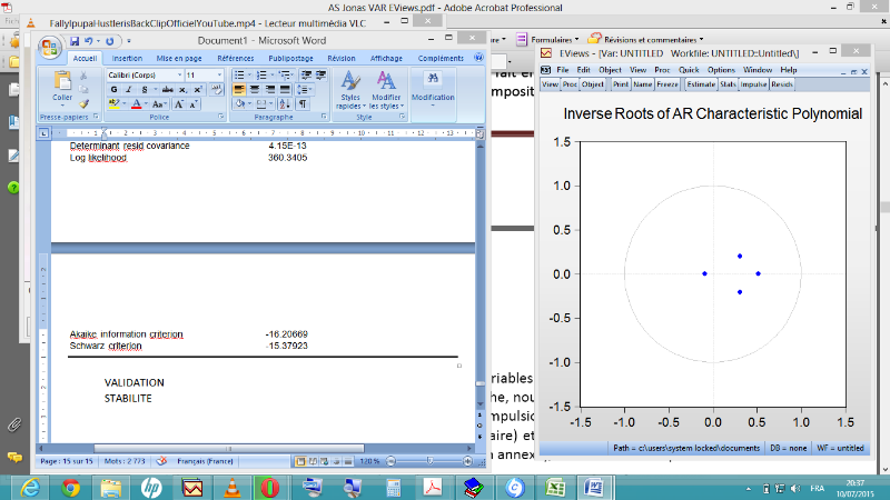
Source : Calculs de l'auteur
à l'aide du logiciel E-views 7
b. Test d'auto corrélation
d'erreurs
Tableau 22 : Test d'auto corrélation
d'erreurs
|
VAR Residual Serial Correlation LM Tests
|
|
Null Hypothesis: no serial correlation at lag order h
|
|
Date: 07/10/15 Time: 20:39
|
|
Sample: 2002Q1 2012Q4
|
|
Included observations: 42
|
|
|
|
|
|
|
|
Lags
|
LM-Stat
|
Prob
|
|
|
|
|
|
|
|
1
|
14.97460
|
0.5265
|
|
2
|
16.57455
|
0.4136
|
|
3
|
15.73225
|
0.4718
|
|
4
|
45.14240
|
0.5341
|
|
5
|
6.628386
|
0.9798
|
|
|
|
|
|
|
|
|
|
|
Probs from chi-square with 16 df.
|
c. Test
d'hétéroscedasticité
Tableau 23 :Test
d'hétéroscedasticité
|
VAR Residual Heteroskedasticity Tests: Includes Cross Terms
|
|
|
Date: 07/10/15 Time: 20:41
|
|
|
|
|
Sample: 2002Q1 2012Q4
|
|
|
|
|
Included observations: 42
|
|
|
|
|
|
|
|
|
|
|
|
|
|
|
|
|
|
|
|
|
|
|
Joint test:
|
|
|
|
|
|
|
|
|
|
|
|
|
|
|
|
|
|
Chi-sq
|
Df
|
Prob.
|
|
|
|
|
|
|
|
|
|
|
|
|
|
|
|
|
125.5734
|
140
|
0.8033
|
|
|
|
|
|
|
|
|
|
|
|
|
|
|
|
|
|
|
|
|
|
|
Individual components:
|
|
|
|
|
|
|
|
|
|
|
|
|
|
|
|
|
Dependent
|
R-squared
|
F(14,27)
|
Prob.
|
Chi-sq(14)
|
Prob.
|
|
|
|
|
|
|
|
|
|
|
|
|
|
res1*res1
|
0.393438
|
1.250942
|
0.2983
|
16.52440
|
0.2824
|
|
res2*res2
|
0.319592
|
0.905862
|
0.5631
|
13.42286
|
0.4935
|
|
res3*res3
|
0.181868
|
0.428715
|
0.9505
|
7.638452
|
0.9073
|
|
res4*res4
|
0.262779
|
0.687431
|
0.7666
|
11.03672
|
0.6831
|
|
res2*res1
|
0.318392
|
0.900874
|
0.5677
|
13.37248
|
0.4974
|
|
res3*res1
|
0.476979
|
1.758800
|
0.1011
|
20.03313
|
0.1291
|
|
res3*res2
|
0.319516
|
0.905546
|
0.5634
|
13.41967
|
0.4938
|
|
res4*res1
|
0.252668
|
0.652036
|
0.7979
|
10.61204
|
0.7162
|
|
res4*res2
|
0.263308
|
0.689309
|
0.7649
|
11.05893
|
0.6814
|
|
res4*res3
|
0.358971
|
1.079986
|
0.4155
|
15.07680
|
0.3729
|
|
|
|
|
|
|
|
|
|
|
|
|
|
|
|
|
|
|
Source : Calculs de l'auteur
à l'aide du logiciel E-views 7
| 

