Zabr modelling

RAPPORT DE STAGE

Diplôme escompté : Master Probabilités et Finance
Entreprise d'accueil: Credit Agricole CIB
Equipe GMD - Structures Rates

présenté et soutenu

par

Kaiza Amuh

le 19 Septembre 2014

Sujet du stage:

Etude du modèle ZABR et du Normal SABR

Maître de stage: Vincent Porte

Jury

M. Emmanuel Gobet, Examinateur

11

iii

Résumé

Dans ce document, nous exposons et résolvons deux problèmes rencontrés par les praticiens avec l'utilisation du modèle SABR : un problème de densité négative et un problème de contrôle des ailes. Pour le premier problème, nous proposons un modèle initialement développé par Philippe Balland, le SABR Normal. Ce dernier permet d'effectuer du pricing sans arbitrage mais présente deux inconvénients majeurs: un temps de calcul excessif et le fait même de changer de modèle de base. Le second problème quant-à lui nous amène à introduite un nouveau modèle, extension du SABR, appelé modèle ZABR. Celui-ci permet de contrôler les ailes du smile grâce à un paramètre particulier mais présente aussi des arbitrages lorsque l'on tente de faire du pricing directement avec les volatilités implicites obtenues en les injectant dans les formules de pricing usuelles de vanilles provenant des modèles de Black-Scholes et de Bachelier. Néanmoins, nous exposons une technique de migration vers un modèle à volatilité locale équivalent au ZABR, essentiellement basée sur de la projection markovienne, qui permet de faire un pricing plutôt "à la Dupire". Ceci permet effectivement d'éviter tout arbitrage, de part la construction même des modèles à volatilité locale. Nous exposons aussi deux façons de calibrer le modèle ZABR, une première assez simple mais peu précise, et une seconde plus fastidieuse découlant du modèle à volatilité locale équivalent au ZABR. Nous faisons ensuite une comparaison des différents temps de calcul et montrons enfin comment le contrôle des ailes de la volatilité implicite peut permettre une couverture plus efficace contre les risques liés à chacun des paramètres du modèle.

iv

Abstract

In this document, we highlight and solve two problems that are encountered by practitioners with the use of the SABR model : a negative density problem and a wings control problem. For the first one, we propose a model initially developed by Philippe Balland, the Normal SABR. The latter allows arbitrage-free pricing but presents two main drawbacks: an excessive computation time and the change of the basis model. The second problem leads to the introduction of a new model, an extension of SABR called ZABR. This one offers a parameter that controls the wings of the smile but also yields arbitrage while attempting a direct pricing with obtained implied volatility, using usual vanilla pricing formulae from Black-Scholes and Bachelier model. However, we expose a trick in order to migrate towards a local volatility model equivalent to ZABR, mainly based on markovian projection, that allows a "Dupire-like" pricing. Doing this completely eliminates arbitrage, because of the very construction of local volatility models. We also present two different ways to calibrate the ZABR model, a first one simple but inaccurate, and a second one which is a direct consequence of the equivalent local volatility modelling and a little bit harder to implement.

v

Acknowledgement

Foremost, I would like to express my sincere gratitude to my advisor Vincent Porte and his colleague Harry Bensusan for their continuous support for my internship, their motivation, enthusiasm, and immense knowledge. Their guidance helped me each time of my research and during the drafting of my report.

Beside my advisor, I would like to thank the whole Structured Rates team of Crédit Agricole, specially Eric N., Thomas T. and Nicolas B. for their availability and their insightful comments.

My sincere thanks also go to all my teachers, specially Emmanuel Gobet, Nicole El Karoui and Vincent Lemaire for their art of dispensing courses very clearly.

ACKNOWLEDGEMENT

? ACKNOWLEDGEMENT

vii

Contents

Résumé ..................................... iii

Abstract ..................................... iv

Acknowledgement ............................... v
Contents ..................................... vii

Introduction 1

1 Problems encountered with SABR model 3

1 Negative density problem ......................... 3

2 Wings Control ............................... 7

2 Normal SABR 11

1 Equivalent SABR local volatility ..................... 12

2 Asymptotic expansion with different base models ........... 13

3 Approximation for normal SABR .................... 15

4 Pricing formula with normal SABR as base ............... 16

3 The ZABR model 21

1 Short maturity expansion ........................ 22

2 Application to benchmark models .................... 24

2.1 Local Volatility model : case ~(ót) = 0 ............. 24

2.2 Degeneracy into a SABR model : case c(ó) = áó ....... 25

3 Expansion for the ZABR model ..................... 26

3.1 Implied volatility computation .................. 26

3.2 Graphical results ......................... 27

3.3 Fast calibration of the model's parameters ........... 29

4 Finite difference volatility ........................ 30

5 Calibrating the Volatility function .................... 32

Conclusion 35

Appendices 35

A Numerical pricing under Normal SABR model 37

1 Density for Normal SABR ........................ 37

2 Computation of functions Ö and ê ................... 38

viii CONTENTS

CONTENTS

B Equivalence between Normal and Log-normal Implied Volatility 41

1 Another pricing formula for call options in the Bachelier model . . . . 42

2 Asymptotics of the implied normal volatility .............. 45

2.1 First and Second order expansion ................ 45

2.2 Accuracy of asymptotic expansions ............... 47

3 Comparing greeks and delta-hedged portfolios ............. 49

Bibliography 53

1

Introduction

European options are often priced and hedged using Black's model, or equivalently, the Black-Scholes model. In Black's model there is a one-to-one relation between the price of a European option and the volatility parameter óLN. Consequently, option prices are often quoted by stating the implied volatility óLN, the unique value of the volatility which yields the option's dollar price when used in Black's model. In theory, the volatility óLN in Black's model is a constant. In practice, options with different strikes K require different volatilities óLN to match their market prices. Handling these market skews and smiles correctly is critical to fixed income and foreign exchange desks, since these desks usually have large exposure across a wide range of strikes. Yet the inherent contradiction of using different volatilities for different options makes it difficult to successfully manage these risks using Black's model.

The development of local volatility models by Dupire [11] and Derman-Kani [10] was a major advance in handling smiles and skews. Local volatility models are self-consistent, arbitrage-free, and can be calibrated to precisely match observed market smiles ans skews. Currently these models are the most popular way of managing smile and skew risk. However, the dynamic behaviour of smiles ans skews predicted by local volatility models is exactly the opposite of the behaviour observed in the marketplace: when the price of the underlying asset decreases, local volatility models predict that the smile shifts to higher prices. In reality, asset prices and market smile move in the same direction. This contradiction between the model and the marketplace tends to de-stabilize the delta and vega hedges derived from local volatility models, and often these hedges perform worse than the naive Black-Scholes' hedges.

To resolve this problem, Hagan, Kumar, Lesniewski and Woodward derived the SABR model, a stochastic volatility model in which the asset price and the volatility are correlated. Singular perturbation techniques are used by the former authors in order to obtain the prices of European options under the SABR model, and from these prices they obtained a closed-form algebraic formula for the implied volatility as a function of today's forward price and the strike. This closed-form formula for the implied volatility allows the market price and the market risks, including vanna and volga risks, to be obtained immediately from Black's formula. It also provides good, and sometimes spectacular, fits to the implied volatility curves observed in the marketplace. More importantly, the formula shows that the SABR model captures the correct dynamics of the smile, and thus yields stable hedges.

2 INTRODUCTION

INTRODUCTION

Why models ? Objectively, it is no good pricing a liquid asset; getting its price directly from the market is largely sufficient. The purpose of models is the pricing of illiquid or scarce assets, such as vanilla options with extreme strikes. Thus, a usable model is one which doesn't break down under extreme conditions. However, SABR model is rather used a reading tool: market data is usually transformed into model parameters through calibration to vanilla assets. Then, the obtained market data (stored as a matrix of SABR parameters) is used for the calibration of more complicated models designed for the pricing of exotic options.

However, since the financial crisis that began in 2007, the american Federal Reserve conducts monetary policy to achieve maximum employment, stable prices, and moderate long-term interest rates. In addition, the Fed purchased large quantities of longer-term Treasury securities and longer-term securities issued or guaranteed by government-sponsored agencies such as Fannie, Mae or Freddie Mac. With such low rates, the SABR model, endowed with Hagan approximation for implied volatility, yields arbitrage. This arbitrage is observable through the negative density of the underlying process.

Furthermore, Interest rate option desks typically need to maintain very large amounts of interlinked volatility data. For each currency, there might be 20 expiries and 20 tenors, that is, 400 volatility smiles. Furthermore, the smiles might be linked across different currencies. Interpolation of observed discrete quotes to a continuous curve is needed for the pricing of general caps and swaptions. At the same time, extrapolation of options quotes are needed for constant maturity swap (CMS) pricing. The SABR model only has four parameters to handle the mentioned tasks, which is not enough flexibility to exactly fit all option quotes.

In this document, we shall outline some problems encountered with SABR model nowadays. We will first solve each problem, then highlight a new model that solves both of our problems.

3

Chapter 1

Problems encountered with SABR

model

Introduction

1 Negative density problem

The industry's standard SABR model (SABR stands for Stochastic-Alpha-Beta-Rho) is a stochastic volatility model defined as follows:

{ dFt = ótFt^âdWt^1 dót = áótdWt^2

with d(W^1, W^2)t = ñdt (1.1)

Where

· ñ E] - 1,1[ represents the link between the forward and its volatility.

· â E [0, 1] is the elasticity of the forward's backbone and is usually assumed constant, requiring then no calibration.

· á > 0 is the parameter that represents the volatility of the volatility process.

Such a model presents a huge advantage because it takes into account the randomness of the volatility parameter of a CEV process. It is then crucial to be able to make a fair pricing under this model. A key is to rather compute a lognormal implied volatility and then plug it into the Black-Scholes formula in order to retrieve the price of the option.

In [26], Hagan et al. used singular perturbation theory and found the following closed form formula for the implied volatility in the SABR model

C z ~

óBS(K, F) = -



(FK)(1-â)/2 (1 + ⁽¹²⁴⁾² log²(F/K) + ^(1-92ô4 log⁴(F/K) + ...) x(z)
ó0

- â)²á² ñâíá2 - 3ñ2 2

C1 + [ (1

24(F/K)1-â + _{4(FK)(1-â)/2} + ₂₄ í ] tex + ...

(1.2)

CHAPTER 1. PROBLEMS ENCOUNTERED WITH SABR MODEL

v1-2ñz+z²+z-ñ

where x(z) = log( 1-ñ ) and z = í á(F K)(1-â)/2 log(F/K)

This formula has the advantage to be fast to compute and, more, is a closed formula. Generally, closed formulas are preferred in the financial industry because of their rapidness and few need of resources.

The same formula could also be obtained applying infinite dimensional analysis and Malliavin calculus. In [34], the author considered a slightly more general model which converges towards the original SABR model and used a large deviation approach based on the non degeneracy of Malliavin covariance. The Dynamic SABR model is rather used for FX Option markets.

Malliavin calculus can be used in a more general scope : the decomposition of a process into consecutive Wiener chaos yields an exact solution to all stochastic differential equations, provided they really have a unique one [...].

However, even though this formula apparently suits to our needs, it produces arbitrage for sufficiently low rates and long maturities. That arbitrage is also observable when â is set to low values.

In order to highlight the arbitrage, let's compute the probability density function of the underlying:

Let pF denote the underlying probability density function (which is then supposed to exist) and PF the corresponding repartition function.

If we compute the price of a call option under the suitable forward probability Q^T, we'd have:

Ct = E^QT ((FT - K)+ ) t

?Ct		?	(FT1{FT >K} - K1{FT >K})
?K =		?K

4

1. NEGATIVE DENSITY PROBLEM

?^2Ct ?K2

= -E^QT(1{FT >K}) t = -Q^T(FT > K) Z +8 = - pF (y)dy K [ ~ ? = PF (K) - lim y?+8 PF (y) ?K

= pF(K)

Where Ct denotes the price of a European call option of strike K, written on the underlying (Ft)t.

Thus, for a set of strikes, we first compute implied volatilities with Hagan formula, then price a set of calls for each strike, and finally compute a numerical derivative of the call price twice according to the strike.

The result is the so-called probability density that we have plotted in the following picture for several maturities.

1. NEGATIVE DENSITY PROBLEM

5

CHAPTER 1. PROBLEMS ENCOUNTERED WITH SABR MODEL



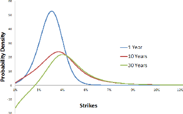
Figure 1.1: F0 = 0.0325, ó0 = 0.087, á = 0.47, â = 0.7, ñ = -0.48

Indeed, as we can see it on the above picture, we may have some negative densities while increasing the option's maturity.

In order to improve the accuracy of the implied volatility approximation, Henry Labordere used a heat kernel expansion on a Riemann manifold endowed with an Abelian connection in [27] and found an approximation for a more general scope of stochastic volatility models. Applying this asymptotic development to SABR model yields:

óN(K,T) = S0(K)(1 + TS1(K)) (1.3)

where

1 _(x l aauñsinh(d(x)) - 1 S0(x)²xF

S0(x) = S(x) log \Fl , 8 (x) _ 4 ^(/Eâ-1) d(x) 28(x)2 log a(x)a(F)xâFâ

_q

á(x^1-â - F 1-â)

q(x) = 1 - â , a(x) = óô + q(x)² + 2ó0ñq(x)

S(x) = 1 _log q(x)

u+ o(1 o-0+p +pp) a(x) d(x) = argch -q(x)ñ - ó0ñ² + a(x)

á ó0(1 - ñ²)

_N/

~ = KF

The above implied volatility is a normal one, i.e. retrieved from an inversion of the pricing formula in the Bachelier Model. For comparison, we can approximately find back a Black-Scholes implied volatility through the following equivalence:

óN =	2 ~S-K ~ 3 V' S - K log KS(log S-log K) 2 2 log S - log K óLN 1 ^-(log S - log K)2 óLNT + O (T log(T) (1.4)

CHAPTER 1. PROBLEMS ENCOUNTERED WITH SABR MODEL

In particular, uN ~ S-K

log S-log K óLN when T ? 0. We gave a detailed proof of this

equivalence in Appendix B.

The following picture shows how Labordere's approximation improves the accuracy of implied volatility asymptotics.



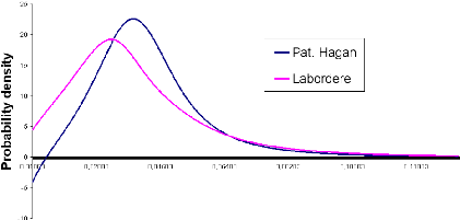
Figure 1.2: F0 = 0.0325, u0 = 0.087, á = 0.47, 9 = 0.7, p = -0.48, T = 15Y

For a 15 years expiry, the negative densities observed with the Hagan expansion simply vanish. Despite that accuracy, for a sake of rigor, we make some model parameters "worse" and track the behaviour of the probability density. We know that a SABR model with parameter 9 = 1 and constant volatility is identically a Black-Scholes model. We can therefore reasonably expect the model to spread from the basic Black-Scholes when 9 ? 0. In the following picture, we choosed 9 = 0.4: let's see what happens.



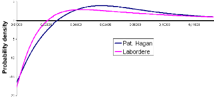
6 1. NEGATIVE DENSITY PROBLEM

Figure 1.3: F0 = 0.0325, u0 = 0.087, á = 0.47, 9 = 0.4, p = -0.48, T = 15Y

CHAPTER 1. PROBLEMS ENCOUNTERED WITH SABR MODEL

As we can remark it, both Hagan and Labordere approximations fail under extreme conditions. This is not really surprising since those formulas are simply short-maturity expansion results. Hence, we address a more qualitative question: which one practitioners prefer between fast to compute approximations and heavy accurate calculus ?

The SABR model can be used to accurately fit the implied volatility curves observed in the marketplace for any single exercise date. More importantly, it predicts the correct dynamics of the implied volatility curves. This makes the SABR model an effective means to manage smile risk in markets where assets only have a single exercise date; these markets include swaption ans caplet/floorlet markets.

2 Wings Control

We now address the issue of wings control. The price of illiquid assets extremely depends on the shape of the implied volatility wings. This is for example the case of the price of a CMS, specially due to the computation of convexity adjustments. A high out-of-money implied volatility yields high prices.

Here is for example how SABR parameters control the smile: The lower we set á, the more we spread the smile...



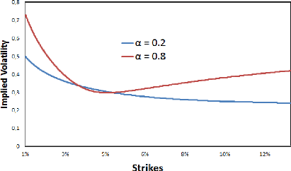
Figure 1.4: F0 = 0.0325, u0 = 0.087, â = 0.7, p = -0.48, T = 15Y

2. WINGS CONTROL 7

The higher we set â, the flatter the smile gets...

8 2. WINGS CONTROL

CHAPTER 1. PROBLEMS ENCOUNTERED WITH SABR MODEL





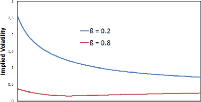
Figure 1.5: F0 = 0.0325, ó0 = 0.087, á = 0.47, p = -0.48, T = 15Y

This is not surprising since for 9 = 1 and a constant volatility, we face a Black-Scholes model and the latter produces nothing but a flat smile !

Increasing p rotates the smile in a counter-clockwise direction.



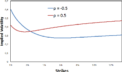
Figure 1.6: F0 = 0.0325, ó0 = 0.087, á = 0.47, 9 = 0.7, T = 15Y

We therefore focus on finding other model parameters, or at least, adapted transformations of SABR model that may provide additional control features.

2. WINGS CONTROL 9

CHAPTER 1. PROBLEMS ENCOUNTERED WITH SABR MODEL

Practitioners usually focus on changing the backbone shape of SABR model, that is, the curve of ATM implied volatilities for different strikes. In order to add more control parameters to the model, we can replace the ?(F) = F'³ in the underlying SDE by:

· ?(F) = F'3(F) with â(F) = â0 + (â₈ - â0) (1 - e-F/Fmax) where Fmax is typically much larger than the forward rate F0. This gives a control on the upper-wing of the smile.

· ?(F) = F'³ x (F/F1)$1+1

(F/F2)$2+1. This parametrisation allows us to control both lower

and upper wings.

· ?(F ) = F $1 1+F$1-$2 .

The later was suggested to me by the Fixed Income Derivatives Quants of Crédit Agricole, and has the particularity to converge to different SABR models. Indeed,

(1.5)

F '31

lim ?(F) = lim = F'32

F?+8 F?+8 1 + F'31-'32

F '31

lim ?(F ) = lim = F '31

F ?0 ?0

F ¹ + F'³¹-'³²

This model tends then to a SABR(â1) for low values of the forward and a SABR(â2) for high forwards.

Despite those improving attempts, practitioners still face a major problem: the above listed backbone transformations lead to a full control of the smile, both liquid and illiquid regions. As highlighted in the introduction, models are needed for illiquid assets; however, models should first behave well for liquid assets for a sake of calibration. If one modifies SABR's behaviour for the whole smile, one although fits illiquid region's behaviour but also loses the liquid region's behaviour. This is therefore a destruction of the cornerstone of our model.

What we need is another model that provides a real parameter for wings control without changing the model's behaviour for liquid assets. We will therefore propose a new model which is able to change wings without (sensibly) touching the liquidity region.

Conclusion

In addition to the negative density problem for very in-the-money vanilla options, the SABR model lacks an additional control parameter for very out-of-money options.

In the next chapter we will expose solutions for both of these problems. We shall develop a Normal SABR model which solves the negative density problem, and then study the ZABR model that controls the wings.

CHAPTER 1. PROBLEMS ENCOUNTERED WITH SABR MODEL

10 2. WINGS CONTROL

11

Chapter 2

Normal SABR

Introduction

As mentioned in the previous chapter, problems with the SABR implementation through the Hagan expansion, such as the breakdown of the expansion for high volatility and the possibility of negative probabilities for very low strikes, did not matter at the time but now constitute a pressing problem for the swap and rates options markets. In this chapter, we present a solution to these problems based on Philippe Balland and Quan Tran expansion (see [7])

The SABR backbone function ?(.) satisfies the usual linear growth and Hölder continuity conditions to ensure that the SABR stochastic differential equation admits a unique solution when appropriate boundary conditions are specified.

In the original dynamics, ?(F) = Fâ and the forward rate is assumed to be absorbed at zero. The constant elasticity of variance (CEV) â is typically greater than zero and smaller than one in interest rate applications. Negative rates can be accommodated by assuming that (Ft + Ä)t follows SABR dynamics. The model is very popular among practitioners because it provides an intuitive parametrisation of volatility smiles.

Unfortunately, the asymptotic formula derived by Hagan et al. (2002) loses accuracy for long-dated expiries, especially when the CEV exponent is close to zero or when the volatility-of-volatility is large. This loss of accuracy is problematic from a practical point of view because the density can become negative near the forward. New techniques have recently been proposed to improve the accuracy in the original expansion of the implied volatility. When the correlation is zero, Antonov & Spector [35] derived an exact expression for the price of a vanilla option based on a double integral. When the correlation is non-zero, the authors proposed using an approximately equivalent SABR model with zero correlation.

Small CEV exponents are typically used to represent swaption and caplet smiles at the long end of the curve, where the asymptotic formula also breaks down. Based on this observation, we perform an asymptotic expansion of the implied volatility corresponding to Normal SABR with absorption at zero, instead of Black-Scholes. We find that the resulting approximation is more accurate than the original SABR

and the measure d Q

dQ

Q except for the drift of ót:

ñt. We note that Jt has the same dynamics under Q and

12 1. EQUIVALENT SABR. LOCAL VOLATILITY

CHAPTER. 2. NOR.MAL SABR.

expansion and results in significant calculation time saving when compared with solving the one-factor equivalent local volatility PDE.

1 Equivalent SABR local volatility

As explained in [15] and [25], we can obtain an accurate approximation of the local volatility equivalent to SABR. The local volatility g(t, K) for SABR is given by the following expression:

g(t, K)² = ?(K)²E [ó2 _t ä (Ft - K)] (2.1)
E [ä (Ft - K)]

We denote the numerator of this expression (the so-called local time) by Lt, and the denominator (the process's probability density) by Dt. In this section, we derive an approximation for g(t, K) by simple applications of Itô's lemma and Girsanov's theorem. We have included this derivation as it will serve as the basis for our normal SABR expansion.

The SABR local time Lt is approximated by introducing the process:

1 du

J(Ft,ót) =ót jFt

(u) (2.2)

and observing that:

Lt = ó0?(K)E [e^áWt2-2tä(Jt)] (2.3)
By applying Itô's lemma and performing the change of measure dbQ

dQ = _eáWt²-2¹á²t,

we derive:

Lt = ó0?(K)

bE [ä(Jt)]

1 (2.4)

dJt = \/q(Jt)d^cWt - 2 ÿ?(Ft)ótdt

where q(J) = 1 - 2ñáJ + á²J² and _(Wt)t is a brownian motion under ^bQ.

The SABR density Dt is similarly approximated by performing the change of

-áWt2-21á2t :

E [ä(Jt)/ót]

D=

?(K)

=

measure dQ

dQ = e

E [ä(Jt)]eá2t

ó0?(K) (2.5)

_p

dJt = q(Jt)d Wt + ÿq(Jt)dt - 21 ÿ?(Ft)ótdt We define the martingale:

dñt ÿq(Jt)

= d W (2.6)
ñt Nq(Jt)

CHAPTER 2. NORMAL SABR

1 !

Z t ÿd(Ju)

Xt = ñt exp ÿ?(Fu)óuq(Ju)du (2.7)

2 0

It follows that the SABR density satisfies:

_i

E hq(J0) _eá²t
q(Jt)ä(Jt)

q(J0)ó0?(K)

Dt =

=

E hexp C2 R0 ^ÿ?(Fu)óu^ÿq_qt du) /Jt = 0i

×

q(J0)ó0?(K)

(2.8)

E [ä(Jt)]

Since the volatility ót only appears in the drift expression of Jt, we conclude that

^bE[ä(Jt)] E[ä(Jt)]

= 1 + O(t²). We consequently have:

g(t, K)² = q(J0)ó20?(K)2e 2 ⁽ñáÿ?(K)-21ÿ?(F0)Z0)⁾t + O(t²) (2.9)

We finally derive the following first-order approximation in time of the SABR local volatility:

_p

g(K) = ó0?(K) 1 + 2ñáf(K) + á²f(K)²,

Z K

1 du (2.10)

f(K) = ó0 ?(u)

F0

Using this equivalent local volatility, we obtain Hagan's first order approximation for the implied volatility under SABR using standard results for local volatility:

ln (K/F0) =(2.11)

R f(K;?) dí

0 v1+2ñáí+á2í2

ln (K/F0)

IV (K; ?, á, ñ) =

RK du
0 g(u)

The SABR local volatility behaves like a CEV dynamic near zero. The absorption at zero is ignored in the above approximation because we are using Black-Scholes as the base model for our implied volatility calculation. Hence, we can expect to improve accuracy by choosing a base model with a dynamic absorbed at zero.

2 Asymptotic expansion with different base models

Suppose that we can accurately integrate the following instance of the SABR dynamics:

? ???? ????

dFt = ót?^base(Ft)dWt^1dót = áótdWt^2 ót=0 = b0

(2.12)

where á and ñ are as in SABR. By matching the first-order implied volatility approximations, that is, IV (K; ?base, á, ñ) = IV (K; ?, á, ñ), we derive the base

2. ASYMPTOTIC EXPANSION WITH DIFFERENT BASE MODELS 13

CHAPTER 2. NORMAL SABR

implied volatility b0 so that the base model and SABR share the same implied volatility to first order in time:

u

ó0(1 - r

JF^K0 (Pbas^de(u)

b0 = (2.13)

K1-â - F1-â

0

We consider two base candidates. Our first one is SABR with shifted lognormal backbone:

?

base 1 (F) = pF + (1 - p)F0 (2.14)
This base dynamics can be integrated by inverting a Laplace transform. Al-

though tractable, this requires a double integration.

Our second candidate is normal SABR with absorption at zero:

?base 2 (F) = lim â?0

Fâ = 1{F>0} (2.15)

We will see in the next section that SABR with a normal backbone can be accurately approximated with limited calculation cost. We observe that the initial normal volatility to use when approximating SABR with this base model is as follows:

ó0(1 - â)(K - F0)

b0 = (2.16)
K1-â - F 1-â

0

In the case where we attempt to approximate SABR with an extended backbone ?(.) instead of a CEV backbone, then our formula for b0 is generalised as follows:

ó0(K - F0)

(2.17)

b0 = _rK du

JF0 ?(u)

As observed in [4], the SABR dynamics calibrated to swaption smiles do not imply Constant Maturity Swap (CMS) levels consistent with the market. Various methods have been proposed to address this issue. These attempts to steepen the upper-strike wing while not affecting the liquid region and the lower wing too much. They are based on modifying either the density, conditionally to being in the upper-wing or directly the SABR dynamics.

We can gain control on the upper-wing steepness by assuming the following backbone:

?(F) = Fâ(F)

F~F~, a~ (2.18)

â(F) = â0 + (â₈- â0)(1 - e- )

where Fmax is typically much larger than the forward rate F0 in order to localise the effect of double beta to the high-strike wing.

An alternative is to use the following double-beta backbone to control both lower and upper wings:

?(F) = F^â x (F/F1)â¹ + 1 (2.19)

(F/F2)â² + 1

14 2. ASYMPTOTIC EXPANSION WITH DIFFERENT BASE MODELS

CHAPTER 2. NORMAL SABR

This parametrisation allows us to account for the extra risk premium for high-strike volatilities and for the fact that traders typically increase â when interest rates become very low.

3 Approximation for normal SABR

We obtain the following formula for a call option under the normal SABR model by applying the Tanaka-Meyer formula to a call payout (see [8]):

T

E[(FT - K)⁺] = (F0 - K)⁺ + 2 J b²₀E [u²_tä(Ft - K)] dt (2.20)

0

where ut = ót/b0 with ó0 = b0. We observe that:

E [u²_t ä(Ft - K) = E [utä(Xt)]

Xt = Ft - K (2.21)

ut

Finally, we denote by Pu the probability measure associated with the Radon derivative ut = ót/b0 and obtain the following formula for a call option under normal SABR:

T

E[(FT - K)⁺] = (F0 - K)⁺ + 2 Z bE^u [ä(Xt)] dt (2.22)

The process _(Xt)t satisfies:

_p

dXt = b0 q(Xt)dW u (2.23)

t?ô

where q(X) = 1 - 2ñáX + á²X², á = á/b0 and r is the first time F hits zero.

The stopping of the diffusion is a consequence of using SABR with vanishing CEV coefficient. As explained in [25], accounting for this stopping is important because the support of SABR is the positive half line and our base model must share with SABR the same behaviour at zero otherwise our lower-strike wing will be too steep. The importance of using interest rate models with absorbing and reflecting boundaries is discussed in [12].

Ignoring the volatility-of-volatility, we approximate r as the first time X hits its expected barrier level under Pu, at which point X_ô = Eu [-K/ut] = -K. This approximation does not compromise the accuracy of our call price because it only affects option prices with very low strikes. We can gain additional control on the lower-wing steepness by assuming that X is absorbed at the level Fmin - K where Fmin = (p - 1)/pF0 is negative, that is, 0 < p < 1.

We define the following process:

!

xt

It = I(Xt) = / du = 1 ln q(Xt) - ñ + áXt (2.24)

o q(u) á 1 - ñ

We can derive an approximation for the density of _(Xt)t at zero using the reflection principle for Brownian motion (see Appendix A):

3. APPROXIMATION FOR NORMAL SABR 15

CHAPTER 2. NORMAL SABR

Eu [ä(Xt)] = q(X0)14

b0 v2ðt

~ ~

e- ^B2

b2 0t - e-

b2

× Ë(t) × 0t

16 4. PRICING FORMULA WITH NORMAL SABR AS BASE

I(F0 - K) 2I(Fmin - K) - I(F0 - K)

B = v2 , C = v2 ~ ~ Ë(t) e- 8 á2t × Ö ^1t, I0 b0 ~ 3 Z t ~ ~ du Ö(t, z) = E exp 8á^2(1 - ñ^2) /Wt = z f(Wu) 0 1 ~(1 + ñ)^2e^-2áW+ (1 - ñ)^2e^2áW+ 2(1 - ñ^2)~ f(W) = 4

(2.25)

Hence, we obtain the following approximation for call prices under SABR:

2 _C2

E[(FT - K)⁺] = (F0 - K)⁺ + q(F0 - K)1/4b0 T1ef0 _,L e° (e b20t - e ^b20t) dt

2v2ð o t

ó0(K - F0) b0 = R K du

F0 ?(u)

ê(t, z) = -₈á² + ?tlnÖ(t, z) 1

(2.26)

The function ê(t, z) is independent of K and only depends on the SABR parameters á and ñ.

~ 1 ~

1 3 1

^{2 2 2}

(2.27)

We have the following first-order approximation:

Ö(t, z) = exp [-¹₈á²t

+ ₁₆á²(1 - ñ2) C f(0) + f(z)/

_t]

+ O(t²)

We can estimate ê(t, z), Ö(t, z) more accurately without any major increase in calculation time. First, we pre-compute by forward induction Ö (Ti,îjvTi) on a fixed-time grid {Ti}i<N and an N(0, 1)-mesh {îj}j<M as explained in Appendix A.

~ ~

Finally, we approximate ê s, ^I0 by a constant êi over each interval _(Ti-1, Ti): b0

êi 1 2 = -8á +	h ~ i h ~ i ln Ö Ti, ^I0- ln Ö Ti-1, ^I0 b0 b0		(2.28)

where Ö(Tk, z) is obtained by cubic spline interpolation of {Ö (Tk, îjvTk) : j = 0,..., M - 1}.

4 Pricing formula with normal SABR as base

From our previous calculations, we derive the following approximation for the price of an option on a SABR underlying _(Ft)t using normal SABR as a base for our asymptotic expansion:

CHAPTER 2. NORMAL SABR

N

E[(FT-K + = (F0 - K)^#177; + q(F0 - K)1/4b é (âa²+~z)Ti 1~ (T Io × J

) ) 2v2ð _o ( Z-1 bo / i

i=1 \

Ji =

1 Z Ti 1 vt 2 Ti-1

~ ~ e- ^B2 eêit b2 0t - e- ^C2 b2 0t dt

(2.29)

The above integrals Ji are calculated using formula (7.4.33) in [20]:

_I

~ ~v ~ ~~

+ e-2|ë|v-ê -êT - |ë|

erf v + 1

T

_T r2 ~_te^êu-û² du ^=Le2|ë|v-ê (erf (-êT + - T(2.30)

where

Z x ~ v ~

2

erf(x) = _?ð e^-t2dt = 2N x 2 - 1 (2.31)

0

and v-ê is either imaginary or real. The error function with complex argument can be estimated using the infinite series approximation of Abramowitz & Stegun (see formula 7.1.29 in [20]) as suggested in [8]:

+8

e

x2 2

-

_n2

-

n2 + 4x2 (f_n(x, y) + ig_n(x, y))

e

4

X

_e-x²

erf(x + iy) = erf(x) + _2ðx (1 - cos 2xy + isin2xy) + ð

n=1

f_n(x, y) = 2x - 2x cosh(ny) cos(2xy) + n sinh(ny) sin(2xy) g_n(x, y) = 2x cosh(ny) sin(2xy) + n sinh(ny) cos(2xy)

(2.32)

In practical application, it is sufficient to include the first 10 terms to ensure a very good accuracy. From the above expression, we can calculate analytical expressions for the cumulative and density functions.

In the following picture, we have plotted the implied density obtained when pricing under Normal SABR. For a sake of comparison, we have also plotted densities obtained from Hagan and Labordere approximations.

4. PRICING FORMULA WITH NORMAL SABR AS BASE 17

18 4. PRICING FORMULA WITH NORMAL SABR AS BASE

CHAPTER 2. NORMAL SABR



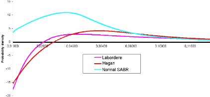
Figure 2.1: F0 = 0.0325, u0 = 0.087, á = 0.47, 9 = 0.4, p = -0.48, 'y = 1, T = 15Y

Indeed, the negative density problem is solved, even for extreme model parameters.

The main drawback is a high computation time, mainly due to the computation of transition probabilities. The latter is however performed once for all strikes.



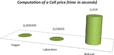
Figure 2.2: F0 = 0.0325, u0 = 0.087, á = 0.47, 9 = 0.4, p = -0.48, 'y = 1, T = 15Y

The above picture shows how much time it actually takes to price under Normal SABR. This pricing takes 200 times more time than the Hagan and Labordere approximations but that is the price we pay in order to eliminate arbitrage.

4. PRICING FORMULA WITH NORMAL SABR AS BASE 19

CHAPTER 2. NORMAL SABR

Conclusion

The Normal SABR model solves the negative density problem observed with the Hagan approximation. However, it introduces another issue, the excessive computation time for pricing. Indeed, practitioners prefer closed form formulas for pricing (such as Black-Scholes) and changing the whole pricing kernel can quickly become a trip to Pandemonium. Moreover, solving only the negative density problem leaves untouched the wings control one. In the next chapter, we will introduce a wings controlling model and show how to compute arbitrage-free prices.

CHAPTER 2. NORMAL SABR

20 4. PRICING FORMULA WITH NORMAL SABR AS BASE

Chapter 3

The ZABR model

Introduction

Interest rate option desks typically need to maintain very large amounts of inter-linked volatility data. For each currency, there might be 20 expiries and 20 tenors, that is, 400 volatility smiles. Furthermore, the smiles might be linked across different currencies. Interpolation of observed discrete quotes to a continuous curve is needed for the pricing of general caps and swaptions. At the same time, extrapolation of options quotes is needed for constant maturity swap (CMS) pricing. For these purposes, the industry uses to approximate SABR model using expansions as in [26]. The implied volatility expansions have the advantages that they are fast and simple to code but as mentioned in the previous chapter, these expansions are not very accurate, particularly not for long maturities nor low strikes.

With the low rates we have today, this problem is more acute than ever. Furthermore, the SABR model only has four parameters to handle the above-mentioned tasks, which is not enough flexibility to exactly fit all option quotes. In this chapter, we extend the stochastic volatility process to include a constant elasticity of variance (CEV) skew on the volatility of volatility. The CEV volatility process allows us to have more explicit control of the extrapolated high-strike volatilities, which in turn allows better control of CMS prices. Further, we will use a non-parametric volatility function for the spot process, which enables us to have an exact fit to all the observed quotes and gives us the ability to model negative option strikes.

In this chapter, instead of buying into heat kernel expansions, we use a short-maturity expansion for the implied volatility of the option. The short maturity expansion also yields results for the short-maturity limit of the Dupire forward volatility ( [11]), that is, the short-maturity limit of the conditional expected local variance

V(F)^2= uim t?0

] dhF it dt /Ft = F (3.1)

21

We provide two procedures to directly calibrate the model to observed CMS prices: an implicit method that works by iteration of the connection from parameters to price in a non-linear solver (see Section 3.3), and a direct method that infers the

22 1. SHORT MATURITY EXPANSION

CHAPTER 3. THE ZABR MODEL

parameters of the model from an arbitrage-free continuous curve of option prices (see Section 5).

1 Short maturity expansion

We consider the slightly more general model:

( dFt = ót?(Ft)dW_t¹

with d(W¹, W²)t = ñdt (3.2)

dót = c(ót)dW_t²

The non-parametric form of the volatility function ?(.) allows us to have a perfect fit to any discrete or continuous set of observed arbitrage-free options quotes. We can write the price of an European call option on a fixing FT as:

Ct = E [(FT - K)⁺ /Ft] = g (t, Ft, v(t))

where v(t) is the implied normal volatility and g is the normal (Bachelier) option pricing formula:

g(ô, x, v) = (x - K)JV x - K + vôfv.Vô)z ^Cv~K) , ô = T - t (3.3)
Applying Itô's lemma to 3.3 yields:

dCt = -g_ôdt + gxdFt +1

gxxd(F)t + gvdvt + _2gvvd(v)t + g_xvd(F, v)t (3.4)
where subscripts denote partial derivatives. In the following, we assume vt > 0 Define Xt = Ft-K. Using Itô's lemma yields:

vt

1 dXt = vt

dFt -Ft 2^Kdvt - 2d(F,v)t + Ft -3Kd(v)t vt vt vt

(3.5)

(3.6)

1

= (dFt - Xtdvt) + O(dt)
vt

d(X)t = v2 (d(F)t + Xt d(v)t - 2Xtd(F, v)t)

t

2

gxx

gxx

The normal option pricing function, g, has the following properties:

g_v = vôgxx

Cx - K

gvv = v

x - K

v

gxv =

1

0 = -g_ô + ₂v²gxx

Using the above properties, we can transform equation 3.4 into:

1. SHORT MATURITY EXPANSION

23

CHAPTER 3. THE ZABR MODEL

1 ]

dCt - gxdFt = 2gxx [v2 t (d(X)t - dt) + 2ôvdvt (3.7)
The left hand side of 3.7 is the change in value of a hedged portfolio. Taking conditional expectations yields:

1

0 = ₂gxxv²

1 t E (d(X)t - dt/Ft) + gxxôvtE (dvt/Ft) (3.8)
For small maturities, ô -+ 0, and we have

₂gxxv²t E (d(X)t - dt/Ft) 0 (3.9)

As gxx > 0 for v > 0, and for any diffusion, E (d(X)t - dt/Ft) = 0 is equivalent to d(X)t = dt, we obtain the arbitrage condition:

d(X)t		= 1 (3.10)	dt

Note that this is a diffusion condition rather than the drift condition that we normally see in financial mathematics. As the function X H X(f, ó) must be a function of the state variables (Ft, ót), the diffusion condition 3.10 leads to the differential equation:

1 = (XfdFt + X_ódót)²

dt (3.11)
= ó²_t ?(Ft)²X²_f + E(ót)²X²_ó + 2ñót?(Ft)c(ót)XfX_ó

Given the function ?(.), we need to solve this non-linear first order differential equation subject to the boundary condition X(f = K, ó) = 0. Once we have the solution X(f, ó), we can find the implied volatility as:

F - K

=

v(3.12) X(F,ó0)

We note that the error of the implied volatility is O(ô). The result implies that for any choice of ?(F), any function X = X(f, ó) that satisfies d(X)t = dt leads to an implied volatility given by v = (F - K)/X.

We could have chosen to derive the short-maturity expansion in implied Black-Scholes (lognormal) volatility v instead of implied normal volatility. Instead of X,

we should then have chosen the transformation

. The diffusion condi-

X = ln(F/K)

v

tion would be the same so X = X. This relates short-maturity implied lognormal and normal volatilities, as in Appendix B (first order equivalence), by the simple relationship:

v ln(F/K)

= (3.13)

v F - K

The expansion results that we present in the following can easily be switched between use in implied normal and implied lognormal volatility form by use of equivalence formulae.

CHAPTER 3. THE ZABR MODEL

2 Application to benchmark models

Before we address the very ZABR model results, we first of all apply the short-maturity expansions from the previous section to well known models. Those models can be retrieved while varying the function c(.).

2.1 Local Volatility model : case ~(ót) = 0

In this case, ót = 1, and the differential equation 3.11 reduces to ordinary differential equation (ODE):

X²_f?(F)² = 1 (3.14)

Using the boundary condition X(F = K) = 0, we find the solution:

Z F 1 X = ?(u) K

du (3.15)

v = v =

with corresponding implied normal and Black volatilities given by:

F - K

f F K ?(u)du

1

(3.16)

ln(F/K)

f F K ?(u)du

1

These results appear in many places, for example in [19]. We note that 3.15 implies the following relationship between X and the forward volatility:

?X ?K =

1 (3.17) ?(K)

Suppose we have X from a stochastic volatility model like 3.2, that is, given as the solution to 3.11 for some volatility functions ?(F), c(ó) and correlation ñ. Let's define the function V by:

~?X ~-1

V(K) = - (3.18)

?K

and consider the deterministic local volatility model:

dFt = V(Ft)dWt (3.19)

It now follows that:

XLV =

Z S K

V(u)^-1du = X (3.20)

24 2. APPLICATION TO BENCHMARK MODELS

So the stochastic volatility model 3.2 and the local volatility model 3.19 will produce the same short-maturity expansion option prices.

The above is a short-maturity limit version of the general result by Gyongy and Dupire (see [13] and [6]), that the model:

CHAPTER 3. THE ZABR MODEL

dFt = a(t, Ft)dWt , F0 = F0 (3.21)

produces the same option prices as the model 3.2 if a(., .) is chosen to be:

~dhF it ~

a(t, k)² = E dt /Ft = k (3.22)

We conclude that in the short-maturity limit, the conditional expected variance of the underlying is related to the transformed variable X by:

-2

V(F)² t~o E [^dh_dti^t/Ft = F~ = (?K\ (3.23)

This constitutes a way of relating the two dimensional pricing problem 3.2 to the simpler one-dimensional pricing problem 3.19. We will make use of this relationship to generate arbitrage-free prices later.

2.2 Degeneracy into a SABR model : case €(ó) = áó

Here, we will solve the diffusion condition for the lognormal volatility process case. First, we use the transformation:

Y :=

_LF

?(u)

1

du (3.24)

and we get:

dY = dW_t¹ - áYdW_t² + O(dt)

= [1 + á2Y 2 - 2ñáY ]1/2 dBt + O(dt) (3.25)
= J(Y )dBt + O(dt)

where _(Bt)t is a new Brownian motion. As Y (F = K) = 0, we can now get X by normalising the volatility of Y , hence:

_fY X=J J(u)^-1du = 1_ln(J(Y ) - ñ + áY\

o 1--p

v =	F - K			(3.26)
ln(F/K) X

For the CEV case ?(F) = ?0Fâ, we have:

1

Y = ó0?0

F1-â - K1-â

(3.27)

1 -â

These formulas are basically the result of Hagan et al [26]. This is extended to include maturity and various refinements for the CEV case. The Hagan result does,

2. APPLICATION TO BENCHMARK MODELS 25

CHAPTER. 3. THE ZABR. MODEL

however, produce implied volatility smiles that are prima facie identical to those produced with formula 3.26.

We can also use 3.26 to retrieve the forward volatility function of SABR from:

?X ?K =

?X ?Y

?Y ?K =

J(Y ) Ç0?(K)) (3.28)

26 3. EXPANSION FOR. THE ZABR. MODEL

Hence:

V(K) = J(Y )ó0?(K) (3.29)

This result could also be deduced from results in [25].

3 Expansion for the ZABR model

We now consider the extended SABR model where the volatility process is of the CEV type: c(ó) = áó^,y

3.1 Implied volatility computation

Once again, we introduce the intermediate variable:

F Y = ó,y-2 1 x ?(u)

du (3.30)

For which Itô expansion yields:

dY = ó,y-1 (dW t 1 + (ã - 2)áYdW ² + O(dt) (3.31)

0 t

Let's define X = ó1-,y

0 f(Y ), for some function f(.), and we get:

dX =ó1-,y

0 f^'(Y)dY + (1 - ã)áf(Y)dW_t² + O(dt)

[ ] t + O(dt) (3.32)

= f'(Y)dW t 1 + (ã - 2)áY f^'(Y) + (1 - ã)áf(Y) dW ²

We conclude that the diffusion condition 3.9 is satisfied if f solves the ODE:

1 = A(Y )f'(Y )^2 + B(Y )f(Y )f^'(Y ) + Cf(Y )2 A(Y ) = 1 + (ã - 2)2á2Y ^2 + 2ñ(ã - 2)áY B(Y ) = 2ñ(1 - ã)á + 2(1 - ã)(ã - 2)á^2Y C = (1 - ã)^2á^2 f(0) = 0 The above ODE can be rearranged as:

(3.33)

f^'(Y ) =

Y -B(Y )f + B(Y )2

f2 - 4A(Y )(Cf² - 1)) F(Y, f) (3.34)

²

CHAPTER 3. THE ZABR MODEL

which can be solved by standard techniques for integration of ODEs. We can evaluate the solution for all strikes one sweep by:

= -ó₀ ?(K)^-1

ã-2

?Y ?K

?K = ó1-ã

0

= -ó^-1

0 F (Y, óã-1

₀ X) ?(K)-1

(3.35)

?X

?f ?K

X(K = F) = Y (K = F) = 0

Again, we can find the forward volatility function as:

/?X\-1= ó0?(K)f'(Y )^-1 = ó0?(K)F (Y, óã-1

₀ X)-1 (3.36)

V(K) = - ?K

Equations 3.35 and 3.36 will typically be evaluated at ó0 = 1. Rather than numerically solving the two ODEs in 3.35 separately, we favour solving 3.33 as a joint system.

It should here be noted that the ODE representation 3.33 has previously been obtained by Balland (see [24]) for the lognormal case. Further, it should be noted that Henry-Labordere has a treatment of the general non-CEV case (see [27]).

3.2 Graphical results

In order to solve the ODE 3.33, we have the choice between a classical Euler scheme and an 4^th order Runge Kutta relaxation. The former is faster but deliver unstable solutions, whereas the latter, even though slower, yields excellent solutions in terms of stability. We therefore chose a RK4 method to solve the ODE. After solving it, we find a value for X which leads to the implied volatility. The following picture plots obtained lognormal implied volatilities for different values of ã.

3. EXPANSION FOR THE ZABR MODEL 27

28 3. EXPANSION FOR THE ZABR MODEL

CHAPTER 3. THE ZABR MODEL



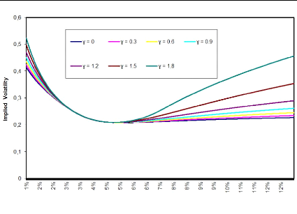
Figure 3.1: F0 = 0.0325, u0 = 0.087, á = 0.47, 9 = 0.7, p = -0.48, T = 15Y

Increasing 'y lifts the wings of the implied volatility smile whereas the smile for strikes close to at-the-money are visibly unaffected. This can in turn be used to give us better control over the CMS prices.

Here is an illustration of how to control CMS prices through the wings. When we increase á, we lift the wings and therefore raise the CMS prices. We can then decrease 'y and therefore lower back the wings and the CMS prices, as we can see it through the following illustration.



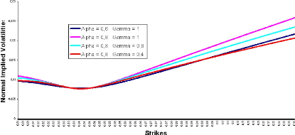
Figure 3.2: F0 = 0.0325, u0 = 0.087, 9 = 0.7, p = -0.48, T = 15Y

In terms of computation time, we have plotted the time it takes to compute an implied volatility in a ZABR('y = 1) and compared it with the time taken by Hagan

CHAPTER. 3. THE ZABR. MODEL

and Labordere approximations.



Figure 3.3: F0 = 0.0325, ó0 = 0.087, á = 0.47, â = 0.7, ñ = -0.48, ã = 1, T = 15Y

It takes 10 times more time for computing implied volatility under the ZABR model, in comparison with Hagan and Labordere approximations. However, this is just the price to pay for gaining control of the wings !

3.3 Fast calibration of the model's parameters

For quick identification of the model parameters, the following second-order Taylor expansion is convenient:

v(K) = v(F) + v^,(F)(K - F) + ¹₂v^,,(F)(K - F)² + O ((K - F)³) v(F) = ó0?(F)

1 v^,(F) =₂ hó₀^-1 ñá + ó0? (F)i

v,,(F) _{6ó0?(F)hó02(7-1)} ((-5 + 2ã)ñ² + 2) + óô (2?(F)?^,,(F) - ?^,(F)²)i

(3.37)

Let's consider a CEV case where we set ?(K) = ù (K-F )â

have:

(F -F )â and ó0 = 1. Then we

v(F) = ù v^,(F) = 21 [~ ñá + Fùâ - F ~~(-5 + 2ã)ñ^2 + 2 á2 + ù^2â(â - 2) ~ v^,,(F) = 1 6ù (F - F)^2 3. EXPANSION FOR. THE ZABR. MODEL

(3.38) 29

CHAPTER 3. THE ZABR MODEL

	\ v(K1), ...,			For a given set of discrete quotes

be used for regressing the triple v(F), v'(F), v"(F). One can in turn solve 3.38 to get parameters estimates for â, ñ, á.

4 Finite difference volatility

Using the implied volatility coming from the short-maturity expansions 3.16, 3.26 and 3.35, directly for pricing using 3.3 will not give arbitrage-free options prices. Our short-maturity expansions suffer from the same problem of potential negative implied densities for low strikes as the original Hagan expansion. The ZABR model contains an enhanced feature that can help us avoid negative density problems. Let's plot the implied probability density function for extreme model parameters and see how it reacts to the changes in ã values.



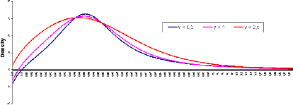
Figure 3.4: F0 = 0.0325, ó0 = 0.087, á = 0.47, â = 0.7, ñ = -0.48, T = 15Y

If we keep increasing ã, the density tends to be more and more positive... Anyway, this way of skipping negative densities doesn't give us enough flexibility in the use of the ZABR model.

In order to definitely avoid this problem, we will instead use the forward volatilities derived in 3.29 and 3.36 as the basis for our pricing.

The forward volatility V(K) can be used to generate option prices as the solution of the Dupire forward PDE (see [5]).

?C(T,K)

?T =

?

?

?

2V(K)2 ?2 ?(T2,K)

C(0, K) = (F - K)⁺

(3.39)

30 4. FINITE DIFFERENCE VOLATILITY

The usual way of solving this numerically is to set up a time discretisation with multiple time steps and then use a finite difference solver. However, to gain speed, we will instead use the single time step implicit finite difference approach introduced in [15]. Here we need to solve the ODE:

C(T, K) - ₂T è(K)2?2C(T, K)

1 ?K2 = (F - K)⁺ (3.40)

4. FINITE DIFFERENCE VOLATILITY 31

CHAPTER 3. THE ZABR MODEL

Z0

It is shown in [15] that this approach generates a set of arbitrage-free call prices for any choice of è. It is also shown that the one-step finite difference price is the Laplace transform of the solution to 3.39. The Laplace transform of the Gaussian distribution is the Laplace distribution:

8 t/T 1 F - Kl T

IF K|

vt

vt

dt = e 2v2 (3.41)

v

v

2v²

which is peaked at K = F. Therefore if we choose è = V, we will also get a peak in the densities.

Instead, we will find an adjustment for the forward volatility function based on our expansion results. As option prices generated by 3.39 and 3.40 should be the

same, we can substitute ?²C(T,K) ?C(T,K)

?K2 = 2 ?T from 3.39 into 3.40 and rearrange to V2

find:

è(K)^2 = V(K)2 C(T, K) - (F - K)^+ T ?C(T,K) ?T V(K)2g(T, F,v) - (Fv) - K)^+ T ?g(T ?T

(3.42)

~ ~

1 - î Ö(-î)

= 2V(K)² , with î= v X

ö(î) T

= V(K)²P(X)²

where the second (approximated) equality involves the approximation of the option prices by our expansion result.

The function P(X)² can conveniently be approximated with a third or fifth order polynomial. Specially:

Ö(X) X

ö(X) a_nuⁿ, u = 1 (3.43) 1 + pX

n

where the constants p, a1, a2, ... can be found in (26.2.16) and (26.2.17) of [20]. The finite difference discretisation of 3.40 is:

~ ~

1- ¹ 2Tè(K)2 ?2 C(T, K) = (F - K)⁺ (3.44)

?K²

This equation can be represented as a tridiagonal matrix equation on the grid K0, K1, ..., K_n, which in turn can be solved for C(T, Ki) in linear CPU time using the tridiag() algorithm in [31].

As an alternative to the finite difference solution 3.44, one could use the exact solution methodology for ODEs of the type 3.40 described in [3]. However, for this methodology to be computationally effective, the forward volatility function è(K) needs to be well approximated by a piecewise linear function with few knot points over the full domain of the solution. This is generally not the case here. We have therefore chosen to base our solution on 3.44.

We can see that the finite difference generated option prices have corresponding implied densities that are positive, that is, arbitrage is precluded. We can also

CHAPTER 3. THE ZABR MODEL

see that using our forward volatility result, V(K), directly in the single time step finite difference solver produces a density that is peaked around at-the-money. This, however, is eliminated when using the adjusted forward volatility è(K).

5 Calibrating the Volatility function

We first consider the case where we have a continuous curve of arbitrage-free option prices. This could for example be produced by Andreasen & Huge interpolation scheme ( [15]) or come from another ZABR model. We can calculate the forward volatility function by the discrete Dupire equation:

è(K)² = ₂C(T, K) - (F - K)+ (3.45)

T ?2C(T,K)

?K²

Using 3.36, we can calibrate the volatility function:

F (Y, óã-1

₀ X) è(K)

?(K) = (3.46)

ó0P(X)

?Y

where X and Y are found from 3.35 as the solution to the ODE system:

ó₀ P (X)

ã-1

?K =

è(K)F (Y, óã-1 0 X)

?X P(X) (3.47)

?K = è(K)

X(K = F) = Y (K = F) = 0

The above ODE system can be solved for all strikes in one sweep. However, typically, we prefer to calibrate directly to the observed discrete quotes. This is done by solving the ODEs in 3.35 and 3.36 and including the one-step finite difference adjustment 3.42:

?Y		óã-2 0
?(K)

?X ?K =

F (Y, óã-1

₀ X)

(3.48)

ó0?(K)

P(X)ó0?(K)

è(K) = F (Y, óã-1

₀ X)

X(K = F) = Y (K = F) = 0

32

5. CALIBRATING THE VOLATILITY FUNCTION

After solving numerically the above system, we can find the option prices using the one-step finite difference algorithm in 3.44. On top of this, we can use a nonlinear solver to calibrate the volatility function ó(K) to observed discrete option quotes. As we get all option prices in one sweep, we can include CMS forwards and option quotes in the calibration without additional computational costs.

CHAPTER 3. THE ZABR MODEL

Even though non-linear iteration is involved, this procedure is very fast. Typically, we can calibrate a non-parametric volatility function with 10 knot points to a given smile in roughly 50 iterations, which takes approximately one millisecond of CPU time.

When it comes to outright pricing speed, the ZABR model is capable of generating 100'000 smiles, each consisting of 256 strikes in approximately seven seconds. It should be stressed that this includes both numerical ODE and finite difference solutions. This is actually faster than direct use of Hagan's SABR expansion, which takes 10 seconds for the same task. The reason for this difference is mainly that one time-step finite difference is faster at producing prices than the Black formula. An alternative to the ZABR model for producing arbitrage-free options prices is the Fourier-based models, found in [2] for example. For a displaced Heston model (see [1]), numerical solution for 100'000 smiles consisting of 256 strikes via the fast Fourier transform with the Black-Scholes formula used as a control variate takes around 18 seconds (see [14]). It should be noted that this type of model is considerably less flexible with respect to fitting discrete quotes and more difficult to implement.

Though we generally use 3.48 in conjunction with a non-linear solver for the calibration, the direct calibration methodology 3.47 is relevant as it admits direct calibration of one ZABR model to another.

The stochastic process _(Xt)t has unit diffusion and thus, in the sense of the short-maturity limit, is normally distributed. So it is natural to use a uniform spacing in X and a non-uniform spacing in K. For this, the ODE system 3.48 can conveniently be transformed to:

?Y			óã-1 0				?K =
F (Y, óã-1 0 X)		?K
ó0?(K)

?X =

(3.49)

F (Y, óã-1

₀ X)

P (X)ó0?(K)

è(K) = F (Y, óã-1

₀ X)

Y (X = 0) = 0, K(X = 0) = F

In our implementation, we solve 3.49 on a uniform X grid to generate and fix a non-uniform strike grid k0, k1, ... , k_n that is used in the numerical solution of 3.48 during calibration and pricing. As a final remark, we note that ODEs in this section typically will be solved at ó0 = 1.

Conclusion for the ZABR model

We have used a simple method to derive short-maturity expansion for forward volatilities from stochastic volatility models. The solution is an ODE that can be solved numerically for all strikes in one sweep. Finally, we used a one-step finite difference scheme to generate option prices. That approach is very fast and it generates arbitrage-free option prices. We have added flexibility to the original SABR model to get an exact fit of all quoted option prices and better control of the

5. CALIBRATING THE VOLATILITY FUNCTION 33

34 5. CALIBRATING THE VOLATILITY FUNCTION

CHAPTER 3. THE ZABR MODEL

wings of the smile for improved CMS pricing. Also, we can add CMS prices to the calibration without additional computational costs.

35

Conclusion

This research internship focused on solving two main problems encountered with the SABR model in the financial industry:

· an arbitrage problem observed through the negative density of the underlying,

· a lack of flexibility in wings control

We first developed the Normal SABR model and solved the negative density problem (Chapter 2). We then solved the wings control problem by another model, the ZABR model, which is just an extension of the SABR model where one replaces the (usually) lognormal volatility process by a CEV volatility process, gaining then a control on the smile's wings through the CEV exponent 'y (Chapter 3). We remarked that a direct use of computed implied volatilities for pricing doesn't yield arbitrage-free prices and we finally used a Markovian Projection and found an equivalent local volatility model that is rather used for pricing.

For each solved problem, we gain accuracy but we pay back a computation time, specially for the Normal SABR model. Anyway, the time lost with the ZABR model is worth the wings control and the arbitrage-free prices obtained. The ZABR model is therefore usable in pricing libraries without additional excessive costs.

Beyond the subjects studied in my internship, as suggested through picture 3.2, one can efficiently hedge against model parameters' risk by using the 'y parameter to thwart the movements of the other model parameters. Here, we did it manually but it can be very interesting to look for particular relationships between 'y and (á, 9, p) in terms of a parametric function that will be calibrated while readjusting the level of 'y according to how the other parameters move. We should therefore look for a stability in the smile shape despite the changes in other parameters of the model. This can be done by matching the slope and the convexity of the obtained smiles around the strike. Numerical resolution yields optimization algorithms.

We can therefore look forward to finding closed form formulas in the ZABR model scope. My idea is to rely on the Labordere's heat kernel expansion on a Riemann manifold; and the research continues...

CONCLUSION

36 CONCLUSION

Appendix A

Numerical pricing under Normal

SABR model

1 Density for Normal SABR

We approximate the density of _(Xt)t at zero, that is, EQ^u [ä(Xt)]. As previously explained, the process _(Xt)t satisfies:

_V

dWt = b0 q(Xt)dW u t?ô

= X0 = F0 - K

where q(X) = 1-2ñáX +á²X², á-á/b0, (W_t^u)t is a zero-drift Brownian motion under Qu, and ô is the first time X hits -K.

This is achieved by defining the following process:

Xt

(I(X)) du = 1ln (V(Xt) - ñ + áX\

_t -- 10Vq(u) á 1 - ñ

1 (1 + ñ)²e^2áI + (1 - ñ)²e^2áI + 2(1 - ñ²)) q(X) = g(I) - 4

The process It - I(Xt) admits the following dynamic:

V b2 01{t<ô}dt

1 + á2X2 t - 2ñáXt

1

dIt = b0dWt?ô - 2

áXt - ñá

37

We define the process At = q(Xt)¹/⁴q(X0)¹/⁴ and observe that:

~ ~

2

dlnAt = dlnñt + -¹ + 31 - ñ á2bo1{t<ô}dt

8 8 q(Xt)

dñt 1

=

ñt 2

áXt - ñá

V1 + á²X²_t - 2ñáXt

b0dWt?ô

The martingale _(ñt)t defines a new measure Qñ and we have:

dIt = b0dW ^Qñ

t?ô

APPENDIX A. NUMERICAL PRICING UNDER NORMAL SABR MODEL

where (W ^Qñ

t )t is a Brownian motion under Qñ.

We observe that:

EQu [ä(Xt)] = q(X0)¹/⁴E^Qu [Atä(Xt)] = q(X0)¹/⁴Ë(t)E^Qñ [ä(Xt)]

[exp (-₈ á2b20(t t?ô 11= EQñ ? ô) + ³á²b²₀(1 -82) _o du g(Iu)du)) /It = 0J

Ignoring the stopping time in above expression for Ë(t) and using áb0 = á, we derive:

Ë(t) e- _a á2t × Ö(t, I0

b0

(:á²(1

¹z) = E^Qñ [exp - ñ2) t f(W?)) /W^Qñ = zJ

1 f(W) = 4 ((1 + ñ)²e^-2áW + (1 - ñ)²e^2áX + 2(1 - ñ²))

where (W ^Qñ

t )t is a Qñ-Brownian motion with initial value zero.

Since Ö(t, z) depends exclusively on ñ and á, this function can be pre-calculated or alternatively approximated as follows:

Ö(t, z) = exp [á²(1 - ñ2) (f(0) + f(z) / t] + O(t²)

We define ê(t, z) = -¹₈á² + ₁³₆á²(1 - ñ2) (f(0) + _f(z)) + O(t)

Since E^Qñ [ä(It)] = E^Qñ [ä(Xt)], we finally derive using the reflection principle for Brownian motions:

EQu [ä(Xt)] = q(X0)1/4

b0 v2ðt

I(F0 - K)

B=

2I(Fmin - K) - I(F0 - K)

_v2 , C = _v2

B2 - C2

× ef0 ê(s,b00)ds × [eTht - e bit

38 2. COMPUTATION OF FUNCTIONS Ö AND ê

2 Computation of functions Ö and ê

We propose a simple algorithm to calculate the functions Ö and ê. Let's choose a time grid {Ti : i = 0, ... , N} such that T0 = 0, TN = T and we simplify the computation of Ö(Ti, B) with the following approximation:

IE [exp

3 ^Tz dul l(z) (₈á²(1 - ñ2) Jo ?(Wu)/ I W_T% = zJ

Then, we calculate Øi : î 7? Öi (îvTi) on a set of symmetric Hermite nodes that appear in the Gauss-Hermite integration. One chooses M = 2m for a symmetric set and {îk : k = 1, ..., M} such that:

APPENDIX A. NUMERICAL PRICING UNDER NORMAL SABR MODEL

E [f(î)] = _XM pkf(îk).

k=1

We can calculate Øi by forward induction:

Øi(îk) E [Øi-1(æTi-1) exp (ëÄTi 1 J /æTi = îkJ exp (1ÄTi 1

40(si-1æTi-1)/ \ ~(siîk)
si =pTi ë = ₁₆á²(1 - ñ²), æt =_NAWt.

The conditional expectation can be analytically computed since æTi-1 and æTi are unit normal variables with correlation

ñi =q Ti .

Let's consider the following function:

Fi-1(z) = Øi-1(z) exp ~

ëÄTi 1



?(si-1z)

Then we have:

~ Øi(îk) = E Fi-1(ñiîk + q1 - 401 exp(ëÄTi₍¹₎)

Using the decomposition of Fi-1(z) in its basis cubic spline functions, we can write:

Fi-1(z) = _XM Fi-1(îj)èj(z). j=1

By integrating the above, we can simplify the former equation as follows:

Øi(îk) =

XM j=1

~ tt ëÄT ëÄTi pkj x Øi-1(S9) ^x exp itt + ?(si-1sj) ?(siîk))

ci(z) = A1i (z - îi)³ + B1i (z -îi) - A0i (z - îi+1)³ - B0i (z - îi+1) Lil0 = îi, L0 = -50, Ui6=M = îi+1, UM = 50.

2. COMPUTATION OF FUNCTIONS Ö AND ê 39

~ ~ _q ~~

pkj = pkj(ñi) = E

⁽ⁱ⁾ èj ñiîk + 1 - ñ2 i æ

where p(i)

kj satisfies _{Pj p}(i)

kj = 1 but can be negative.

A crucial observation for time saving is the fact that the pseudo-transition proba-

bilities pkj only depends on the mesh îk and the grid Ti. Consequently, the respective

expectations only need to be computed once.

We can analytically calculate the pseudo-transition probabilities. The function

èj is a cubic spline with value zero at every node except at z = îj where it takes

value 1.

èj(z) = _XM 1{Li<z<Ui}ci(z),

i=1

APPENDIX A. NUMERICAL PRICING UNDER NORMAL SABR MODEL

where A0i, B0i, A1i, B1i are calculated using the standard cubic spline algorithm. We finally compute the pseudo-transition probabilities:

pkj(ñ) = _XM ñ³? _[A1iI3(li, ui, vi) - A0iI3(li, ^ui, vi+1)] + ñ? _[B1iI1(li, ui, vi) - B0iI1(li, ^ui, _vi+1)] , i=0

Li - ñîk li = (1 - ñ2)1/2, ui =

Ui - ñîk (1 - ñ2)1/2, vi =

ñîk - îi p (1 - ñ2)1/2, ñ? = 1 - ñ2

Where I_n(a, b, c) = E [1{a<î<b}(î + c)ⁿ]. By integration, we obtain:

I1(a, b, c) = c [N (b) - N(a)] + f_z(a) - f_z(b)

I3(a, b, c) = (c² + 3c)[N(b) - N(a)] + [3c(c + a) + a² + 2] f_z(a) - [3c(c + b) + b² + 2] f_z(b)

where fZ(.) is the Gaussian density.

40 2. COMPUTATION OF FUNCTIONS Ö AND ê

41

Appendix B

Equivalence between Normal and

Log-normal Implied Volatility

Asymptotics of implied volatility are important for different reasons. On the one hand, they give information on the behaviour of the underlying through the moment formula [29] or the tail-wing formula [30]. On the other hand, they allow a full correspondence between vanilla prices and implied volatilities. With such a correspondence, asymptotics in call prices can be easily transformed into asymptotics in implied volatilities. When applied to a specific model, asymptotics are widely used as smile generators [26]. In practice, other models are then used for pricing options using tools like Monte-Carlo simulations.

So far, all the asymptotics studied by authors concern asymptotics for implied lognormal volatility. In this chapter, we consider implied normal volatility which refers to the Bachelier model. Why is it interesting to consider normal implied volatility? One the one hand, for short maturities, the Bachelier process makes more sense than the Black-Scholes model. Indeed, the behaviour of the underlying from one day to another is generally well approximated by a Gaussian random variable [32]. That's the reason why the Bachelier model is very popular in high frequency trading [21]. On the second hand, the "breakeven move" of a delta-hedged option is easily interpreted as normal volatility. Generally, the P&L of a book of delta-hedged option is positive if the (historical) volatility of the underlying is greater than a breakeven volatility which has to be expressed in normal volatility. Moreover, it makes more sense to compare implied normal volatilities with historical moves of the underlying as can be done by a market risk department. Likewise, some markets such as fixed-income markets with products like spread-options are quoted in terms of implied normal volatility [16]. Finally, the skewness of swaption prices is much reduced if priced in terms of normal volatility instead of lognormal volatility. Therefore, it is important to have a robust and quick way to compute implied normal volatilities from market prices and also to be able to switch between lognormal volatilities and normal volatilities.

What kind of asymptotics should we consider? Most of the approximations in option pricing theory are made under the assumption that the maturity is either small (see the Hagan et al. formula [26]) or large [17]; it is actually assumed that

42 1. ANOTHER PRICING FORMULA FOR CALL OPTIONS IN THE BACHELIER MODEL

APPENDIX B. EQUIVALENCE BETWEEN NORMAL AND LOG-NORMAL IMPLIED VOLATILITY

a certain time-variance U²T is either small or large. A possible way to derive such approximations is to replace the factor of volatility U by EU and then set E = 1. This can be done at the partial differential equation level (see all the techniques coming from physics [26]) as well as directly at the stochastic differential equation level with the help of the Wiener chaos theory for instance [33]. Other types of asymptotics are obtained by considering large strikes. In our approach, we unify all those types of asymptotics (see [18] and [9] for the lognormal case). Indeed, we obtain an approximation of the implied normal volatility as an asymptotic expansion in a parameter À for À « 1 and it turns out that À -+ 0 when T -+ 0 or K -+ +00.

This study is organized as follows. We first give another expression for the pricing of a European call option which involves an incomplete Gamma function (Proposition 1.1). Then, we inverse this function asymptotically and obtain an expansion of normal implied volatility. This is particularly important if we want to quickly obtain the implied normal volatilities from call prices as is the case in high frequency trading [21]. The formula is also potentially useful theoretically if, given an approximation for the price of a European call option or a spread option (for instance in the framework of the Heston or the SABR model), we want to obtain an approximation of the normal implied volatility. Finally, we restrict our formula to the order 0 and we compare it to a similar formula for the lognormal case. Then, we obtain an equivalence between normal volatility and lognormal volatility. We use it also to compare the Black-Scholes greeks to the Bachelier greeks. Finally, we consider a delta-hedged portfolio and we compute the breakeven move in the normal case as well as in the lognormal case.

1 Another pricing formula for call options in the Bachelier model

In the Bachelier model, the dynamic of a stock _(St)t?R+ is given by:

( dSt = UNdWt,

(B.1) S0 = S

The so-called normal volatility UN is related to the price of a call C(T, K) struck at K with maturity T by the following formula:

(S - K ) (S - K )

\/

C(T, K) = (S - K) \/ + UN T f_z \/ ,

UN T UN T

(B.2)

( ) Z x

1 _-x²

with f_z(x) = _\/2ð exp and (x) = fZ(u)du.

2 -8

Following Ropper-Rutkowski [23], we can isolate the volatility UN in the pricing formula.

APPENDIX B. EQUIVALENCE BETWEEN NORMAL AND LOG-NORMAL IMPLIED VOLATILITY

Definition 1.1. Let us denote by TV (K,T) (or simply TV ) the time-value of a European call option struck at strike K with maturity T. Then TV (T, K) := C(T, K) - (S - K)+ .

Proposition 1.1. In the Bachelier model, we

TV (T, K) =

{

1 (S-K)^2 if K =6S, 4vð 2^, 2ó^2NT v óN v2ð otherwise T

(B.3)

where (a, z) is the incomplete Gamma function:



(a, z) =

+8

ua-1 exp(-u)du

_f

v

Proof. We have C(T,K)

S = f(î, è) with î := K S and è := óN S and

T

f(î,u) := (1 - î)N \1 - î /u + ufz \1 u
By differentiation, we have:

?u(î,u)=-(1u2î)2fz \1u/+- _îfzu- î_u 1 --

2

_u2¹

/ \ u/fz\1u/

fz

\1 -î/

u

where we have used fz(î) = -îf_z(î). Since f(î, 0) = C(0,K)

S = (1 -î)+ , we

deduce that:

f(î,è) = (1 -î)+ + _fB /1 u

fz ( I du

o \ If we set

F(î, è) :=f^B fz ( \1 u du

o

then we have:

C(T, K) S

Kv ! = (1 - î)+ + F S , ó T S

Let's assume that both è =6 0 and î =6 1. With the change of variable v := 1-î

_u ,

we get:

+8 F(î,è) = |1 -î| f1 î| è

fz(v) dv v2

So, with a new change of variable u := ¹₂v², we have:

1. ANOTHER PRICING FORMULA FOR CALL OPTIONS IN THE BACHELIER MODEL 43

APPENDIX B. EQUIVALENCE BETWEEN NORMAL AND LOG-NORMAL IMPLIED VOLATILITY

Z +8 1 F(î, è) = 4vð |1 - î| ~2 2è

u-

3 2 exp(-u)du

4vð1 |1 - î|(-¹₂,|¹_2è2|²₎

v2ð

where (a, z) is the incomplete Gamma function. At the money, we simply have C(T, K) = óNvT

It's clear from Proposition 1.1 that the real-valued function T 7? C(T, K) is non-decreasing, positive, C(0, K) = (S - K)+ and _limT?+8 C(T, K) = +8. So, given the price of a European call option C, there is a unique real number óN(T, K) such that C(T, K) = C with a normal volatility óN = óN(T, K). We say that óN(T, K) is the normal implied volatility

Remark 1.1. We can easily see that _|Ks| depends only on ^arKT (only one variable).

One of the interests of Proposition 1.1 is that there are efficient algorithms to compute the inverse of the incomplete Gamma function. In particular, it is implemented in Matlab. Therefore, it is always easy to get the implied normal volatility from call prices [22]. Such a task is not always easy in the lognormal case [28], especially when we are far from the money.

Corollary 1.1. Let p be an integer. Then,

(ó

TV T K) = NT) 2 ex _(S - K)2 p-1 1 k (2k + 1)! óNT ^k + R

TV( v2ð(S - K)2 p ( _2ó2NT ) ( ) k! ((S - K)2) p

k=0

with |R_p| = (2p + 1)! 011¹011^1P

p! ( (S - K)2 )

(B.4)

The above equation comes naturally from a well known asymptotic expansion of (a, z) for large z (see Formula 6.5.32 in [20]).

Remark 1.2. From either pricing formula B.2 or B.3, we can notice that we can use the same trick to price large strike and short maturity European options (as expansions in both cases are similar)... This comes from the fact that:

C(ë²T, ëS + (1 - ë)K) = ëC(T, K) for any non-negative real ë. This is particular to the Bachelier model.

For a comparison with the lognormal case, it can be advantageous to introduce the following notations.

44 1. ANOTHER PRICING FORMULA FOR CALL OPTIONS IN THE BACHELIER MODEL

APPENDIX B. EQUIVALENCE BETWEEN NORMAL AND LOG-NORMAL IMPLIED VOLATILITY

Definition 1.2. For K 6=, we set èN := óN s T xN := -1, ãN := log (4vð),

uN :=

|xN |

2è2 - 1

log(TV (T,K)

N

_S ).

x

Then by Corollary 1.1, for K =6 S and p ? N^*,

4vð		TV (T, K)	= u	3/2 e N	1 uLN	X p-1 k=0	(1)^kk k 2k aLNuLN + RpLN
|xN|		S

(B.5)

(B.6)

~

2 /

with uLN := ~LN, èLN := óLNV ^T, xLN := log C S , R^p_LN ? Ù (èx) , xLN

1 x2 i

^LN and(2k + 1)!! := 11(2j + 1).

j!(2j + 1)!! 8

aLkN := (2k + 1)!! _Xn

k=0

j=0

Here, óLN denotes the lognormal implied volatility.

2 Asymptotics of the implied normal volatility 2.1 First and Second order expansion

-

3/2

1 u_N

u

X p-1 k=0

N e

Let us assume that K =6 S. Using B.5, we get:

ukuN + O (u_N))

= eãNe-1/ë

with uk :=

(-1)^k 2k ak

Therefore, by Lemma 1 of [9], we get the following proposition.

Proposition 2.1. Let us denote by TV the time-value of a European call option, óN its implied normal volatility and T the maturity of the option. Set ë := - 1

log(T SV ),

ãN := log

(4_|x,z)

and xN = KS - 1. Let's assume that K =6S. Then, in the case when T ? 0, we have the following expansion for the time-variance of the call option: ó²_NT = (S-K)2

₂ uN with

³_²_²⁹_³_²/⁹ _ \ 3 log(A)

+ (ã²_N -³₂ãN + 2) A3 + o(ë³) (B.7)

In the lognormal case [9], for short expiries, the asymptotic expansion of ó2LNT is

2. ASYMPTOTICS OF THE IMPLIED NORMAL VOLATILITY 45

APPENDIX B. EQUIVALENCE BETWEEN NORMAL AND LOG-NORMAL IMPLIED VOLATILITY

given by ó2LNT = log2(K/S)

2 uLN with

99

uLN =ë - ₂ë²log(ë) +ãLNë² + ₄ë³log²(ë) + 14 - 3ãLN I ë3log(ë)

(N - ë3 + o(ë³)

+ ₂ãLN - u₁ (B.8)

LN := log

XLN 2

-

ã

4vðex ² and ui:= - LN| 16 2

First, we note that ë = uLN + o(uLN). Then comparing the two results B.7 and B.8 for K =6 S, we obtain:

uN = uLN + (ãN - ãLN)u²LN + O (u3LN log(uLN))

So,

~SxN 2

_ó2 LNT + O ~T² log(T)~ (B.9)

N = ó²_LN + 2(ãN - ãLN)S2x2 Nó4

xLN x4 _LN

Since ^xN xLN

S-K = log(S)-log(K) > 0, we deduce that

~ 1/2

SxN

óN =

xLN

SxN

=

xLN

1 + 2(ãN - ãLN)ó2 ^LN + O ~T² log(T)~

óLN T

x2 _LN (B.10)

2 1/2

ó

ã

-ã

^ó

x



LN (1 + (

N

LN)

2NT) + O (T2 log(T))

LN

46 2. ASYMPTOTICS OF THE IMPLIED NORMAL VOLATILITY

Moreover, we have:

Hence, we get: K

ãN - ãLN =

~xLN ~ xLN 2 + log xN

S

? ~S-K ~ ?

-

log ,/KS(log S-log K) ?+ O ~T 2 log(T)~

óN = log(S) - log(K)óLN _?1 - (log S - log K)2 ó2 LNT

Note also that at the money, the situation is quite easy. On the one hand, we have (cf. Proposition 1.1)

_r

2ð

óN = T C

On the other hand, we have ( [9], Proposition 2.1):

v !

óLN T

C = erf 2v2

Therefore, we state the following result.

APPENDIX B. EQUIVALENCE BETWEEN NORMAL AND LOG-NORMAL IMPLIED VOLATILITY

Corollary 2.1.
· if K =6 S, we have:

UN =	2 S-K S - ^KULN 1 - log KS(log S-log K) U2 T + O (T^2 log(T) log S - log K (log S - log K)2 LN

(B.11)

In particular, UN ~

S-K

log S-log KULN when T ? 0.

· At the money, we have UN = /2ðerf óLNT and UN

SULN 1 aLNT

2v2=- +

24

o(T).

In particular, UN ~ SULN when T ? 0.

Remark 2.1. When K ? S, we can check that In other terms, for K =6 S,

S-K log vKS(log S-log K) 1 (log S-log K)^2 24

ULN =

S(m m1) UN, where m = S = xN + 1 is the Moneyness. (B.12) This formula was known (even if it was not stated explicitly) in the SABR model (see Hagan et al. formula [26] ). By differentiatinf Formula B.12 with respect to m, it turns out that the Black-Scholes skew ?óLN

?m at the money (m = 1) generated by

the Bachelier model is ?óLN

?m = _-1 óN S (ULN is by definition the implied lognormal 2

volatility). Therefore, the Bachelier model is highly skewed ATM (a slope of -50%× óNS ). Another way to explain this feature is that given call prices, when we use the BS model, the function ULN is a decreasing and convex function of m, i.e., it generates a skew, while the function UN is a rather flat function of m. Thus, normal volatility is most suited for products such as swaptions for instance.

2.2 Accuracy of asymptotic expansions

Here we address the question of the accuracy of our expansions. Therefore, we proceed by backward induction of the lognormal implied volatility as described bellow:

· Let's choose several random lognormal implied volatility and compute a Call price through Black & Scholes formula without interest rate

· From each Call price, we calibrate the volatility parameter from a Bachelier model by numerical inversion of the pricing formula. We therefore obtain the likely "true" normal implied volatilities equivalent to our initial lognormal volatilities

· For comparison, we respectively apply the first and second order approximations with our initial lognormal implied volatilities and we obtain other normal volatilities that we can compare with the former ones

Applying the above process leads to the following curve where we have plotted comparison curves for different maturities.

The first order approximation supposes an affine relationship between normal and lognormal implied volatilities whereas the second order supposes a parabolic one. We can observe that the raise of the maturity deteriorates our asymptotic expansions. The more we increase the option's expiry, the more our approximation is credible.

2. ASYMPTOTICS OF THE IMPLIED NORMAL VOLATILITY 47

48 2. ASYMPTOTICS OF THE IMPLIED NORMAL VOLATILITY

APPENDIX B. EQUIVALENCE BETWEEN NORMAL AND LOG-NORMAL IMPLIED VOLATILITY



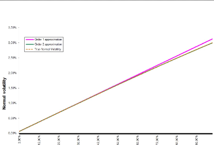
- Order 1 approximation

- Order 2 approximation --- True Normal Volatility

2,50% -

2,90% -

ô ô

V

3,50% -

3,00% -

Lognormal volatility

Figure B.1: T = 1, F₀ = 0.0325, K = 0.03



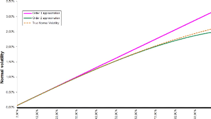
- Order 1 approximation

- Order 2 approximation --- True Normal Volatility

3,09%

3,50%

2,50%

2,99%

0,59%

0,0C%

V V V

ô ô ô ô ô

N N N N

V

Lognormal volatility

Figure B.2: T = 1, F₀ = 0.0325, K = 0.03

APPENDIX B. EQUIVALENCE BETWEEN NORMAL AND LOG-NORMAL IMPLIED VOLATILITY



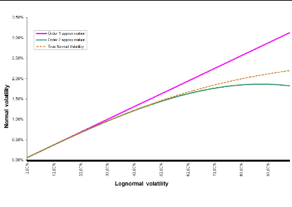
Figure B.3: T = 1, F0 = 0.0325, K = 0.03

3 Comparing greeks and delta-hedged portfolios

Let's denote by ON, FN, íN, ÈN (resp. OLN, FLN, íLN, ÈLN), the delta, gamma,

vega and theta in the Bachelier (resp. Black-Scholes) model. For instance, íN = ?C

?óN .

By differentiating B.2, we get:

CS - K)

ON = N (B.13)

óN vT

On the other hand, it is known that:

OLN = _NClnS - lnK 1 1

+ (B.14)

óLNv T 2ULN T)

So, by Corollary 2.1, we get: OLN ~ ON for a maturity T « 1. By differentiating B.13, we obtain:

ü fz CS ) (B.15)
FN =

óN T óN T

In the Black-Scholes model, we have:

= 1 ClnS - lnK 1 )

FLN SóLNvT fz óLNvT + ₂óLNvT (B.16)

Hence, with the help of Corollary 2.1,

lnS - lnK

FN ~ S - K FLN (B.17)

Now we consider the Vega. It is shown above that:

3. COMPARING GREEKS AND DELTA-HEDGED PORTFOLIOS 49

APPENDIX B. EQUIVALENCE BETWEEN NORMAL AND LOG-NORMAL IMPLIED VOLATILITY

C(T, K) = (S - K)+ + S 0

v óN T S

f(1 - K/S ) ^zu du

So, differentiating w.r.t. óN, we get:

/ (S - K)²

íN T = S 2ð 2T 2~² T ) (B.18)

N

In contrast, the vega in the Black-Scholes model id

/T ((lnS - lnK +₂óTNT)²)

íLN = S _2ð exp (B.19)

2ó2 LNT

Likewise, we can compare the two thetas. We then have the following proposition

Proposition 3.1. When T ? 0, and under the hypothesis of bounded volatilities, we have:

ÄN ~ ÄLN íN ~ íLN N S lnS - lnK LN ~ S - K S - K ÈN ~ ÈLN S(lnS - lnK)^ÈLN

(B.20)

The first equivalence ÄN ~ ÄLN shows that hedging in the Bachelier framework is more or less like hedging in a Black-Scholes framework. However, the "breakeven move" of a delta-hedged portfolio is not the same. By definition, the "breakeven move" of a delta-hedged portfolio is the number u such that over a short horizon ät, P&L > 0 if the change in S is > u. In general, we have:

(ÄS)²

1

=

2

1

P &L = -Èät + 2

[(ÄS)² - u²]

(B.21)

So, with ät = 1,

m - ₁uN (B.23)

lnm

uLN =

with m = K/S. So, at the money, uLN ~ uN. However, if K < S (resp. K > S)

then uLN < uN (rep. uN > uLN.

50

3. COMPARING GREEKS AND DELTA-HEDGED PORTFOLIOS

_r

2È

u = .(B.22)

Using Proposition 3.1, we find that the "breakeven move" uLN in the Black-Scholes model is related with the "breakeven move" uN in the Bachelier model by:

3. COMPARING GREEKS AND DELTA-HEDGED PORTFOLIOS 51

APPENDIX B. EQUIVALENCE BETWEEN NORMAL AND LOG-NORMAL IMPLIED VOLATILITY



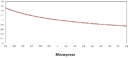
Figure B.4: The volatility smile of the Bachelier model (normalized by the factor óN S where óN denotes the normal volatility

and the ratio of "breakeven moves" uLN/uN.

The following graph represents the function in 7? ln(m)

m-1 which gives the smile

of the Bachelier model (cf Corollary 2.1) as well as the ratio of "breakeven moves" uLN .

uN

So, depending on the view of the trader on the short term dynamic of the underlying (normal or lognormal diffusion), he will adjust or not the "breakeven move"

of his delta-hedged portfolio by the factor lnm

m-1.

APPENDIX B. EQUIVALENCE BETWEEN NORMAL AND LOG-NORMAL IMPLIED VOLATILITY

52 3. COMPARING GREEKS AND DELTA-HEDGED PORTFOLIOS

53

Bibliography

[1] Lipton A. A closed-form solution for options with stochastic volatility with applications to bond and currency options. Review of Financial Studies, 6, 1993.

[2] Lipton A. The vol smile problem. Risk February, 2002.

[3] Lipton A. and A. Sepp. The vol smile problem. Risk February, 2011.

[4] Jesper Andreasen and Brian Huge. Expanded forward volatility. Risk Magazine, 2013.

[5] Dupire B. Pricing with a smile. Risk January, 1994.

[6] Dupire B. A unified theory of volatility. Working paper, BNP Paribas, 1996.

[7] Philippe Balland and Quan Tran. Sabr goes normal. Risk Magazine, 2013.

[8] Eric Benhamou and Olivier Croissant. Local time for the sabr model: Connection with complex black scholes and application to cms and spread options. Working Paper, 2007.

[9] Grunspan C. Asymptotic expansions of the lognormal implied volatility: A model free approach. Preprint, 2011.

[10] E. Derman and I. Kani. Stochastic implied trees: Arbitrage pricing with stochastic term and strike structure of volatility. Int J. Theoritical and Applied Finance, 1998.

[11] B. Dupire, M.A. H. Dempster, and S. R. Pliska. Pricing and hedging with smiles, in mathematics of derivative securities. Cambridge University Press, 1997.

[12] Robert Goldstein and William Keirstead. On the term structure of interest rates in the presence of reflecting and absorbing boundaries. Working Paper, 1997.

[13] Gyongy I. Mimicking the one-dimensional marginal distributions of processes having an itô differential. Probability Theory and Related Fields, 71, 1986.

[14] Andreasen J. and L. Andersen. Volatile volatilities. Risk December, 2002.

[15] Andreasen J. and B. Huge. Volatility interpolation. Risk March, 2011.

54 BIBLIOGRAPHY

BIBLIOGRAPHY

[16] Kienitz J. and Wittke M. Option valuation in multivariate sabr models - with an application to the cms spread. Preprint, 2010.

[17] Fouque JP., Papanicolaou G., Sircar R., and Solma K. Singular perturbations in option pricing. SIAM Journal on Applied Mathematics, 63(5), 2003.

[18] Gao K. and Lee R. Asymptotics of implied volatility to arbitrary order. Preprint, 2011.

[19] Andersen L. and R. Ratcliffe. Extended libor market models with stochastic volatility. Working paper, General Re Financial Products, 2002.

[20] Abramowitz M. and Stegun IA. Handbook of mathematical functions. Dover, 1966.

[21] Avellaneda M. and Stoikov S. High-frequency trading in a limiot order book. Quantitative Finance, 8(3), 2008.

[22] Li M. and Lee K. An adaptative successive over-relaxation method for computing the black-scholes implied volatility. Quantitative Finance, 2009.

[23] Roper M. and Rutkowski M. A note on the behaviour of the black-scholes implied volatility close to expiry. International Journal of Theoretical and Applied Finance, 12(4), 2009.

[24] Balland P. Forward smile. Presentation, ICBI Global Derivatives, 2006.

[25] Doust P. No arbitrage sabr. Working paper, Royal Bank of Scotland, 2010.

[26] Hagan P., Kumar D., Lesniewski A., and Woodward D. Managing smile risk. Wilmott Journal, pages 84 108, Jul 2002.

[27] Henry-Labordere P. Analysis, geometry and modeling in finance. Chapman and Hall, 2008.

[28] Jaeckel P. By implication. Wilmott Journal, nov 2006.

[29] Lee R. The moment formula for implied volatility at extreme strikes. Mathematical Finance, 14(3), Jun 2004.

[30] Benaim S. and Friz P. Smile asymptotics ii: models with known moment generating functions. Journal of Applied Probability, 45(1):16 32, 2008.

[31] Press W., B. Flannery, S. Teukolsky, and W. Vetterling. Numerical recipes in c. Cambridge University Press, 1992.

[32] Schachermayer W. and Teichmann J. How close are the option pricing formulas of bachelier and black-merton-scholes? Mathematical Finance, 18(1):155 170, 2008.

[33] Osajima Y. General asymptotics of wiener functionals and application to mathematical finance. Preprint, 2007.

BIBLIOGRAPHY 55

BIBLIOGRAPHY

[34] Osajima Yasufumi. The asymptotic expansion formula of implied volatility for dynamic sabr model and fx hybrid model. Mitshubishi UFJ Securities Co., 2007.

[35] Osajima Yasufumi. General short-rate analytics. Risk Magazine, 2011.