ANNEXE
Graphe 1 - Base monétaire
|
50000
40000
30000
20000
10000
0
|
|
|
97 98 99 00 01 02 03 04 05 06 07
|
BASEM ON
Graphe 2 - le taux de change
|
45 40 35 30 25 20 15 10
|
|
|
97 98 99 00 0 1 02 03 04 05 0 6 07
|
TAUXCHANGE
Graphe 3- total des credits
|
900 800 700 600 500 400 300
|
|
|
97 98 99 00 01 02 03 04 0 5 0 6 07
|
Graphe 4 - Dépôts gourdes et
dépôts dollars
|
35000
30000
25000
20000
15000
1
0000
5000
0
|
|
|
97 98 99 00 01 02 03 04 05 0 6 07
|
|
DEPDOLL DEPGDES
|
Graphe 5 - Variation mensuelle de l'IPC
|
.1 4 .12 .10 .08 .06 .04
.02 .00 -.02
|
|
|
97 98 99 00 0 1 02 03 04 05 0 6 07
|
IPC
Graphe 6 - Le niveau de l'inflation (sept 96 - oct
07)
|
45 40 35 30 25 20 15 10
5
|
|
|
97 98 99 00 0 1 02 03 04 0 5 0 6 07
|
INFLATION
Graphe 7- Taux sur les bons BRH
|
28 24 20 16 12
8
4
|
|
|
97 98 99 0 0 0 1 02 03 04 0 5 0 6 07
|
TAUXBON
Tableau 1 - le taux de change (Gdes/ $ 1 U.S)
|
janv
|
fev
|
mar
|
avr
|
mai
|
juin
|
juil
|
auot
|
sept
|
oct
|
nov
|
dec
|
|
1996
|
|
|
|
|
|
|
|
|
|
15.55
|
15.27
|
15.09
|
|
1997
|
16.26
|
16.11
|
16.51
|
16.69
|
16.82
|
16.76
|
16.49
|
16.75
|
16.95
|
17.41
|
16.87
|
17.31
|
|
1998
|
17.56
|
17.38
|
17.34
|
16.95
|
16.69
|
16.30
|
16.07
|
16.51
|
16.85
|
16.30
|
16.59
|
16.50
|
|
1999
|
16.78
|
16.89
|
16.68
|
16.69
|
16.70
|
16.70
|
16.82
|
16.80
|
16.94
|
17.55
|
17.96
|
17.97
|
|
2000
|
18.26
|
19.18
|
19.74
|
19.73
|
19.67
|
20.38
|
20.87
|
21.63
|
28.33
|
23.58
|
23.89
|
22.52
|
|
2001
|
23.76
|
23.55
|
23.96
|
23.47
|
23.52
|
24.37
|
24.11
|
24.42
|
25.49
|
26.01
|
25.96
|
26.34
|
|
2002
|
26.67
|
27.20
|
26.77
|
26.68
|
26.97
|
27.28
|
28.44
|
28.76
|
29.70
|
32.95
|
37.27
|
37.61
|
|
2003
|
41.51
|
44.52
|
42.22
|
42.30
|
40.54
|
42.86
|
42.71
|
41.22
|
42.03
|
41.96
|
42.82
|
42.08
|
|
2004
|
44.09
|
43.00
|
40.22
|
37.74
|
36.95
|
35.74
|
36.03
|
36.10
|
36.82
|
37.16
|
37.48
|
37.23
|
|
2005
|
37.69
|
37.89
|
38.20
|
39.03
|
38.70
|
39.92
|
42.08
|
42.34
|
43.04
|
43.03
|
43.06
|
43.00
|
|
2006
|
43.48
|
42.98
|
42.69
|
41.10
|
39.02
|
39.86
|
39.95
|
38.86
|
39.13
|
39.13
|
39.00
|
37.59
|
|
2007
|
38.98
|
38.32
|
37.42
|
36.90
|
36.57
|
35.74
|
35.64
|
35.76
|
36.38
|
|
|
|
TABLEAU 2- le taux d'inflation (%)
|
janv
|
fev
|
mars
|
avr
|
mai
|
juin
|
juil
|
aout
|
sept
|
oct
|
nov
|
dec
|
|
1996
|
|
|
|
|
|
|
|
|
|
15.71
|
14.56
|
14.61
|
|
1997
|
15.07
|
15.19
|
16.87
|
16.38
|
16.65
|
16.89
|
17.25
|
17.59
|
16.95
|
16.68
|
15.92
|
15.59
|
|
1998
|
15.71
|
14.82
|
12.81
|
12.79
|
11.87
|
10.91
|
9.74
|
9.13
|
8.27
|
7.50
|
8.02
|
7.45
|
|
1999
|
7.38
|
7.93
|
7.94
|
7.45
|
7.61
|
8.12
|
8.74
|
9.32
|
9.92
|
10.10
|
9.66
|
9.67
|
|
2000
|
10.02
|
10.45
|
12.00
|
12.29
|
11.88
|
11.49
|
11.65
|
12.52
|
15.32
|
18.03
|
18.96
|
18.98
|
|
2001
|
18.57
|
18.08
|
16.29
|
16.19
|
16.86
|
16.71
|
15.99
|
15.03
|
12.34
|
9.52
|
8.63
|
8.15
|
|
2002
|
7.99
|
8.03
|
8.47
|
8.51
|
8.37
|
8.41
|
8.91
|
9.54
|
10.07
|
11.91
|
12.78
|
14.77
|
|
2003
|
28.88
|
33.25
|
36.96
|
39.25
|
40.57
|
41.66
|
42.03
|
41.92
|
42.46
|
41.23
|
41.49
|
40.43
|
|
2004
|
25.83
|
22.64
|
20.83
|
25.37
|
25.09
|
24.08
|
23.04
|
22.38
|
22.53
|
21.98
|
20.56
|
20.21
|
|
2005
|
19.79
|
18.64
|
17.16
|
12.60
|
12.61
|
14.47
|
15.04
|
16.00
|
14.84
|
15.24
|
15.90
|
15.30
|
|
2006
|
14.50
|
15.30
|
15.30
|
15.10
|
14.20
|
13.00
|
12.60
|
12.20
|
12.40
|
11.80
|
10.70
|
10.30
|
|
2007
|
9.60
|
8.60
|
8.00
|
8.00
|
8.30
|
9.10
|
7.90
|
7.60
|
7.90
|
|
|
|
Tableau 3 - les taux sur les bons de 91 jours
(%)
|
janv
|
fev
|
mar
|
avr
|
mai
|
juin
|
juil
|
auot
|
sept
|
oct
|
nov
|
dec
|
|
1996
|
|
|
|
|
|
|
|
|
|
-
|
19.40
|
17.20
|
|
1997
|
15.70
|
15.30
|
18.10
|
18.60
|
18.00
|
18.00
|
17.90
|
17.70
|
16.30
|
16.40
|
17.20
|
20.50
|
|
1998
|
25.40
|
25.40
|
25.40
|
25.40
|
25.40
|
25.40
|
23.30
|
21.30
|
19.70
|
12.10
|
9.20
|
9.80
|
|
1999
|
10.20
|
10.30
|
10.20
|
10.20
|
10.30
|
10.30
|
10.30
|
10.30
|
15.30
|
17.80
|
21.10
|
21.10
|
|
2000
|
21.10
|
23.30
|
23.30
|
23.30
|
23.30
|
23.30
|
20.70
|
20.70
|
20.70
|
20.70
|
20.70
|
20.70
|
|
2001
|
20.70
|
20.70
|
20.70
|
26.70
|
26.70
|
26.70
|
26.70
|
26.70
|
26.70
|
20.10
|
19.90
|
18.90
|
|
2002
|
16.90
|
15.00
|
12.00
|
10.10
|
9.90
|
10.00
|
10.10
|
10.20
|
10.30
|
10.30
|
15.60
|
15.60
|
|
2003
|
15.60
|
24.40
|
27.80
|
27.80
|
27.80
|
27.80
|
27.80
|
27.80
|
27.80
|
27.80
|
27.80
|
27.80
|
|
2004
|
27.80
|
|
|
22.20
|
22.20
|
20.00
|
20.00
|
13.60
|
7.60
|
7.50
|
7.60
|
7.60
|
|
2005
|
7.60
|
7.60
|
7.60
|
7.60
|
7.60
|
13.40
|
13.40
|
13.40
|
15.60
|
18.90
|
18.90
|
18.90
|
|
2006
|
18.90
|
18.90
|
18.90
|
18.90
|
18.90
|
17.80
|
17.80
|
17.80
|
17.80
|
17.80
|
16.70
|
16.70
|
|
2007
|
16.70
|
16.70
|
15.60
|
14.50
|
14.50
|
13.40
|
13.30
|
9.00
|
8.70
|
|
|
|
Tableau 4: Résultat des tests de la Racine
unitaire
Null Hypothesis: IPC has a unit root
Exogenous: Constant
Lag Length: 0 (Automatic based on SIC, MAXLAG=1)
t-Statistic Prob.*
Augmented Dickey-Fuller test statistic -7.506745
0.0000
Test critical values: 1% level -3.481217
5% level -2.883753
10% level -2.578694
*MacKinnon (1996) one-sided p-values.
Augmented Dickey-Fuller Test Equation
Dependent Variable: D(IPC)
Method: Least Squares
Date: 10/02/02 Time: 01:05
Sample(adjusted): 1996:12 2007:09
Included observations: 130 after adjusting endpoints
|
Variable
|
Coefficient
|
Std. Error t-Statistic
|
Prob.
|
|
IPC(-1)
|
-0.611841
|
0.081505 -7.506745
|
0.0000
|
|
C
|
0.007435
|
0.001460 5.092944
|
0.0000
|
|
R-squared
|
0.305673
|
Mean dependent var
|
6.99E-05
|
|
Adjusted R-squared
|
0.300249
|
S.D. dependent var
|
0.0 14735
|
|
S.E. of regression
|
0.0 12326
|
Akaike info criterion
|
-5.939007
|
|
Sum squared resid
|
0.019446
|
Schwarz criterion
|
-5.894891
|
|
Log likelihood
|
388.0355
|
F-statistic
|
56.35122
|
|
Durbin-Watson stat
|
2.051730
|
Prob(F-statistic)
|
0.000000
|
Null Hypothesis: TB has a unit root
Exogenous: None
Lag Length: 0 (Automatic based on SIC, MAXLAG=1)
t-Statistic Prob.*
Augmented Dickey-Fuller test statistic -7.305058
0.0000
Test critical values: 1% level -2.583593
5% level -1.943406
10% level -1 .615024
*MacKinnon (1996) one-sided p-values.
Augmented Dickey-Fuller Test Equation
Dependent Variable: D(TB)
Method: Least Squares
Date: 10/02/02 Time: 01:07
Sample(adjusted): 1997:02 2007:09
Included observations: 125
Excluded observations: 3 after adjusting endpoints
Variable Coefficient Std. Error t-Statistic Prob.
|
TB(-1)
|
-0.751617
|
0.102890 -7.305058
|
0.0000
|
|
R-squared
|
0.299916
|
Mean dependent var
|
-0.735945
|
|
Adjusted R-squared
|
0.299916
|
S.D. dependent var
|
19.97855
|
|
S.E. of regression
|
16.71626
|
Akaike info criterion
|
8.478609
|
|
Sum squared resid
|
34649.73
|
Schwarz criterion
|
8.501235
|
|
Log likelihood
|
-528.9130
|
Durbin-Watson stat
|
1.734391
|
Null Hypothesis: M2 has a unit root
Exogenous: Constant
Lag Length: 0 (Automatic based on SIC, MAXLAG=1)
t-Statistic Prob.*
Augmented Dickey-Fuller test statistic -11.86448
0.0000
Test critical values: 1% level -3.481217
5% level -2.883753
10% level -2.578694
*MacKinnon (1996) one-sided p-values.
Augmented Dickey-Fuller Test Equation
Dependent Variable: D(M2)
Method: Least Squares
Date: 10/02/02 Time: 01:08
Sample(adjusted): 1996:12 2007:09
Included observations: 130 after adjusting endpoints
|
Variable
|
Coefficient
|
Std. Error t-Statistic
|
Prob.
|
|
M2(-1)
|
-1.043154
|
0.087922 -11.86448
|
0.0000
|
|
C
|
1.106388
|
0.169377 6.532098
|
0.0000
|
|
R-squared
|
0.523749
|
Mean dependent var
|
0.016157
|
|
Adjusted R-squared
|
0.520028
|
S.D. dependent var
|
2.34 1640
|
|
S.E. of regression
|
1.622288
|
Akaike info criterion
|
3.820817
|
|
Sum squared resid
|
336.8728
|
Schwarz criterion
|
3.864933
|
|
Log likelihood
|
-246.3531
|
F-statistic
|
140.7658
|
|
Durbin-Watson stat
|
1.909202
|
Prob(F-statistic)
|
0.000000
|
Null Hypothesis: CRED has a unit root
Exogenous: Constant
Lag Length: 0 (Automatic based on SIC, MAXLAG=1)
t-Statistic Prob.*
Augmented Dickey-Fuller test statistic -1 0.14367
0.0000
Test critical values: 1% level -3.481217
5% level -2.883753
10% level -2.578694
*MacKinnon (1996) one-sided p-values.
Augmented Dickey-Fuller Test Equation Dependent Variable:
D(CRED)
Method: Least Squares
Date: 10/02/02 Time: 01:09
Sample(adjusted): 1996:12 2007:09
Included observations: 130 after adjusting endpoints
|
Variable
|
Coefficient
|
Std. Error t-Statistic
|
Prob.
|
|
CRED(-1)
|
-0.891257
|
0.087863 -10.14367
|
0.0000
|
|
C
|
1.163183
|
0.241524 4.816007
|
0.0000
|
|
R-squared
|
0.445633
|
Mean dependent var
|
0.038029
|
|
Adjusted R-squared
|
0.441302
|
S.D. dependent var
|
3.272695
|
|
S.E. of regression
|
2.446212
|
Akaike info criterion
|
4.642223
|
|
Sum squared resid
|
765.9457
|
Schwarz criterion
|
4.686339
|
|
Log likelihood
|
-299.7445
|
F-statistic
|
102.8941
|
|
Durbin-Watson stat
|
1.970929
|
Prob(F-statistic)
|
0.000000
|
Null Hypothesis: TXC has a unit root
Exogenous: Constant
Lag Length: 0 (Automatic based on SIC, MAXLAG=1)
t-Statistic Prob.*
Augmented Dickey-Fuller test statistic -1 2.42572
0.0000
Test critical values: 1% level -3.481217
5% level -2.883753
10% level -2.578694
*MacKinnon (1996) one-sided p-values.
Augmented Dickey-Fuller Test Equation
Dependent Variable: D(TXC) Method: Least Squares
Date: 10/02/02 Time: 01:10 Sample(adjusted): 1996:12 2007:09
Included observations: 130 after adjusting endpoints
|
Variable
|
Coefficient
|
Std. Error t-Statistic
|
Prob.
|
|
TXC(-1)
|
-1.092346
|
0.087910 -12.42572
|
0.0000
|
|
C
|
0.823786
|
0.383004 2.150856
|
0.0334
|
|
R-squared
|
0.546740
|
Mean dependent var
|
0.027257
|
|
Adjusted R-squared
|
0.543199
|
S.D. dependent var
|
6.370029
|
|
S.E. of regression
|
4.305317
|
Akaike info criterion
|
5.772844
|
|
Sum squared resid
|
2372.577
|
Schwarz criterion
|
5.816960
|
|
Log likelihood
|
-373.2348
|
F-statistic
|
154.3984
|
|
Durbin-Watson stat
|
1.977074
|
Prob(F-statistic)
|
0.000000
|
Vector Autoregression Estimates
|
Date: 05/28/08 Time: 15:53
Sample(adjusted): 1997:02 2007:09
Included observations: 125
Excluded observations: 3 after adjusting endpoints Standard
errors in ( ) & t-statistics in [ ]
|
|
|
|
CRED
|
IPC
|
M2
|
TB
|
TXC
|
|
CRED(-1) 0.236254
|
0.000980
|
0.160919
|
1.005831
|
0.390458
|
|
(0.14166)
|
(0.00064)
|
(0.09040)
|
(0.96633)
|
(0.24792)
|
|
[ 1.66772]
|
[ 1.52937]
|
[ 1.78014]
|
[ 1.04088]
|
[ 1.57496]
|
|
IPC(-1) 39.66389
|
0.334092
|
26.18289
|
47.84967
|
39.57288
|
|
(18.1239)
|
(0.08194)
|
(11.5651)
|
(123.630)
|
(31.7178)
|
|
[ 2.18848]
|
[ 4.07710]
|
[ 2.26396]
|
[ 0.38704]
|
[ 1.24766]
|
|
M2(-1) 0.056646
|
0.001449
|
-0.116764
|
1.283891
|
0.171384
|
|
(0.14325)
|
(0.00065)
|
(0.09141)
|
(0.97713)
|
(0.25069)
|
|
[ 0.39545]
|
[ 2.23730]
|
[-1 .27741]
|
[ 1.31394]
|
[ 0.68366]
|
|
TB(-1) -0.003613
|
0.000203
|
0.003376
|
0.225726
|
0.002762
|
|
(0.01508)
|
(6.8E-05)
|
(0.00962)
|
(0.10284)
|
(0.02638)
|
|
[-0.23964]
|
[ 2.98244]
|
[ 0.35097]
|
[ 2.19489]
|
[ 0.10468]
|
|
TXC(-1) -0.142283
|
-0.000210
|
-0.038071
|
0.169990
|
-0.336910
|
|
(0.07928)
|
(0.00036)
|
(0.05059)
|
(0.54079)
|
(0.13874)
|
|
[-1 .79473]
|
[-0.58589]
|
[-0.75257]
|
[ 0.31434]
|
[-2.42833]
|
|
C 0.579521
|
0.005065
|
0.720570
|
-3.737150
|
-0.034648
|
|
(0.34183)
|
(0.00155)
|
(0.21813)
|
(2.33174)
|
(0.59822)
|
|
[ 1.69536]
|
[ 3.27750]
|
[ 3.30347]
|
[-1.60273]
|
[-0.05792]
|
|
R-squared 0.062985
|
0.285449
|
0.079848
|
0.103917
|
0.056614
|
|
Adj. R-squared 0.023614
|
0.255426
|
0.041186
|
0.066266
|
0.016976
|
|
Sum sq. resids 698.5436
|
0.014280
|
284.4384
|
32504.01
|
2139.414
|
|
S.E. equation 2.422832
|
0.010954
|
1.546040
|
16.52704
|
4.240079
|
|
F-statistic 1.599796
|
9.507635
|
2.065291
|
2.760032
|
1.428270
|
|
Log likelihood -284.9101
|
389.9594
|
-228.7550
|
-524.9176
|
-354.8657
|
|
Akaike AIC 4.654561
|
-6.143350
|
3.756080
|
8.494682
|
5.773851
|
|
Schwarz SC 4.790320
|
-6.007591
|
3.891839
|
8.630441
|
5.909610
|
|
Mean dependent 1.284466
|
0.011693
|
1.082287
|
-0.195409
|
0.826600
|
|
S.D. dependent 2.451955
|
0.012695
|
1.578896
|
17.10344
|
4.276533
|
|
Determinant Residual
|
3.020506
|
|
|
|
|
Covariance
|
|
|
|
|
|
Log Likelihood (d.f. adjusted)
|
-955.9256
|
|
|
|
|
Akaike Information Criteria
|
15.77481
|
|
|
|
|
Schwarz Criteria
|
16.45360
|
|
|
|
Graphique 7 : Fonction des reponses impulsionnelles
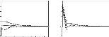

Response to Cholesky One S.D. Innovations #177; 2 S.E.
Response of TB to TB
Response of TB to TB Response of TB to M2 Response of TB to CRED
Response of TB to TXC Response of TB to IPC
Response of TB to M2
Response of TB to CRED
Response of TB to TXC
Response of TB to IPC
20
20
20
20
20

16
16
16
16
16
12
12
12
12
12
8
8
8
8
8
4
4
4
4
4
0
0
0
0
0
-4
-4
-4
-4
-4
1 2 3 4 5 6 7 8 9 10 11 12
1 2 3 4 5 6 7 8 9 10 11 12 1 2 3 4 5 6 7 8 9 10 11 12 1 2 3 4 5 6
7 8 9 10 11 1 1 2 3 4 5 6 7 8 9 10 11 12 1 2 3 4 5 6 7 8 9 10 11 12
1 2 3 4 5 6 7 8 9 10 11 12
1 2 3 4 5 6 7 8 9 10 11 1
1 2 3 4 5 6 7 8 9 10 11 12
1 2 3 4 5 6 7 8 9 10 11 12
Response of M2 to TB
Response of M2 to M2
Response of M2 to CRED
Response of M2 to TXC
Response of M2 to IPC
Response of M2 to TB Response of M2 to M2 Response of M2 to CRED
Response of M2 to TXC Response of M2 to IPC
2.0
2.0
2.0
2.0
2.0

1.6
1.6
1.6
1.6
1.6
1.2
1.2
1.2
1.2
1.2
0.8
0.8
0.8
0.8
0.8
0.4
0.4
0.4
0.4
0.4
0.0
0.0
0.0
0.0
0.0
-0.4
-0.4
-0.4
-0.4
-0.4
-0.8
-0.8
-0.8
-0.8
-0.8
1 2 3 4 5 6 7 8 9 10 11 12
1 2 3 4 5 6 7 8 9 10 11 12 1 2 3 4 5 6 7 8 9 10 11 1 1 2 3 4 5 6
7 8 9 10 11 12 1 2 3 4 5 6 7 8 9 10 11 12 1 2 3 4 5 6 7 8 9 10 11 12
1 2 3 4 5 6 7 8 9 10 11 1
1 2 3 4 5 6 7 8 9 10 11 12
1 2 3 4 5 6 7 8 9 10 11 12
1 2 3 4 5 6 7 8 9 10 11 12
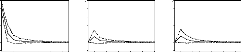
Response of CRED to TB
Response of CRED to M2
Response of CRED to CRED
Response of CRED to TXC
Response of CRED to IPC
Response of CRED to TB Response of CRED to M2 Response of CRED to
CRED Response of CRED to TXC Response of CRED to IPC
2.8 2.4 2.0 1.6 1.2 0.8 0.4 0.0 -0.4
2.8 2.4 2.0 1.6 1.2 0.8 0.4 0.0 -0.4
2.8 2.4 2.0 1.6 1.2 0.8 0.4 0.0 -0.4
2.8 2.4 2.0 1.6 1.2 0.8 0.4 0.0 -0.4
2.8 2.4 2.0 1.6 1.2 0.8 0.4 0.0 -0.4


-0.8
-0.8
-0.8
-0.8
-0.8
1 2 3 4 5 6 7 8 9 10 11 12
1 2 3 4 5 6 7 8 9 10 11 12 1 2 3 4 5 6 7 8 9 10 11 12 1 2 3 4 5 6
7 8 9 10 11 12 1 2 3 4 5 6 7 8 9 10 11 12 1 2 3 4 5 6 7 8 9 10 11 12
1 2 3 4 5 6 7 8 9 10 11 12
1 2 3 4 5 6 7 8 9 10 11 12
1 2 3 4 5 6 7 8 9 10 11 12
1 2 3 4 5 6 7 8 9 10 11 12
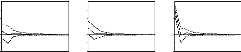
Response of TXC to TB
Response of TXC to M2
Response of TXC to IPC
Response of TXC to TB Response of TXC to M2 Response of TXC to
CRED Response of TXC to TXC Response of TXC to IPC
Response of TXC to CRED
Response of TXC to TXC
4
4
4
4
4


3
3
3
3
3
2
2
2
2
2
1
1
1
1
1
0
0
0
0
0
-1
-1
-1
-1
-1
-2
-2
-2
-2
-2
1 2 3 4 5 6 7 8 9 10 11 12
1 2 3 4 5 6 7 8 9 10 11 12 1 2 3 4 5 6 7 8 9 10 11 12 1 2 3 4 5 6
7 8 9 10 11 12 1 2 3 4 5 6 7 8 9 10 11 12 1 2 3 4 5 6 7 8 9 10 11 1
1 2 3 4 5 6 7 8 9 10 11 12
1 2 3 4 5 6 7 8 9 10 11 12
1 2 3 4 5 6 7 8 9 10 11 12
1 2 3 4 5 6 7 8 9 10 11 1
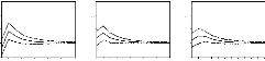
Response of IPC to TB
Response of IPC to M2
Response of IPC to CRED
Response of IPC to TXC
Response of IPC to IPC
Response of IPC to TB Response of IPC to M2 Response of IPC to
CRED Response of IPC to TXC Response of IPC to IPC
.012
.012
.012
.012
.012


.008
.008
.008
.008
.008
.004
.004
.004
.004
.004
.000
.000
.000
.000
.000
-.004
-.004
-.004
-.004
-.004
1 2 3 4 5 6 7 8 9 10 11 12
1 2 3 4 5 6 7 8 9 10 11 12
1 2 3 4 5 6 7 8 9 10 11 1
1 2 3 4 5 6 7 8 9 10 11 12
1 2 3 4 5 6 7 8 9 10 11 12
| 

