Impact du réchauffement climatique sur la distribution spatiale des ressources halieutiques le long du littoral français: observations et scénarios( Télécharger le fichier original )par Sylvain Lenoir Université Lille 1 Science - Doctorat 2011 |

1.5. ConclusionLe nouveau modèle NPPEN, appliqué à l'échelle de l'Atlantique Nord, est capable de fournir des cartes de distribution spatiale de l'espèce Gadus morhua, et ce avec l'avantage de n'avoir besoin que des données de présence. Ce modèle étant non-paramétrique, il s'affranchit également du besoin de normalité des variables. Le NPPEN explique la chute prononcée de l'abondance de la morue en mer du Nord depuis les années 1960. Il se révèle ainsi très utile pour évaluer les changements futurs de la répartition géographique des espèces, dans le contexte du changement climatique, en fonction de scénarios d'évolution du climat. Ce modèle constitue un nouvel outil d'aide à la gestion durable des stocks de la morue de l'Atlantique. 2. Publication: A new model to assess the probability of occurrence of a species based on presence-only dataA new model to assess the probability of occurrence of a species based on presence-only data G. Beaugrand, S. Lenoir, F. Ibañez, C. Manté Marine Ecology Progress Series, 2011.(In press) This study aims to describe a new nonparametric ecological niche model for the analysis of presence-only data, which we use to map the spatial distribution of Atlantic cod and project the potential impact of climate change on this species. The new model, called the Non-Parametric Probabilistic Ecological Niche (NPPEN) model is derived from a test recently applied to compare the ecological niche of two different species. The analysis is based on a simplification of the Multiple Response Permutation Procedures (MRPP) using the Generalised Mahalanobis distance. For the first time, we propose to test the generalized Mahalanobis distance by a non-parametric procedure so avoiding the arbitrary selection of quantile classes to allow the direct estimation of the probability of occurrence of a species. The model NPPEN was applied to model the ecological niche (sensu Hutchinson) of Atlantic cod and therefore its spatial distribution. The modelled niche exhibited high probabilities of occurrence at bathymetry ranging from 0 to 500 m (mode between 100 m and 300 m), at annual sea surface temperature from -1°C to 14°C (mode between 4°C and 8°C) and at annual sea surface salinity ranging from 0 to 36 (mode between 25 and 34). This made the species a good indicator of the subarctic province. Current climate change is having a strong effect on North Sea cod and may have also reinforced the negative impact of fishing on stocks located offshore of North America. The model shows a pronounced effect of current climate change on the spatial distribution of Atlantic cod. Projections for the coming decades suggest that cod may eventually disappear as a commercial species from regions where a sustained decrease or collapse has already been documented. In contrast, the abundance of cod is likely to increase over the Barents Sea. Keywords: Ecological Niche Models; Multiple Response Permutation Procedure; Generalised Mahalanobis distance; Ecological niche; The Atlantic cod The effects of climate change on living systems in both the terrestrial and the marine realms are now well documented (Parmesan & Matthews 2006, Intergovernmental Panel on Climate Change 2007a). In the marine biosphere, current climate change is affecting the abundance, spatial distribution and the phenology of species and altering prey-predator interactions (Beaugrand et al. 2002, Beaugrand et al. 2003, Edwards & Richardson 2004). The effect of climate change is seen from phytoplankton (Reid et al. 1998) to zooplankton (Beaugrand et al. 2007) and fish (Brander et al. 2003, Perry et al. 2005), and translates from the physiological to the ecosystem level (Pörtner & Farrell 2008) affecting coupling between systems (i.e. bentho-pelagic coupling; (Reid & Edwards 2001, Kirby et al. 2008). Pronounced climate change may become a confounding factor of fishing and both driving forces may act in synergy to precipitate the collapse of fish stocks around the world (Beaugrand & Kirby 2010b, a). To better evaluate the effect of climate on a species, it is essential to know its spatial distribution; this information is often lacking in the marine realm. One way to evaluate the spatial distribution of a species is to use Ecological Niche Models (ENMs). ENMs, also known as bioclimatic envelopes, are being more frequently used in the context of global change and are often based on the concept of the ecological realised niche described by Hutchinson (Hutchinson 1957). The realised niche is the environmental envelop in which a species can be found when the effect of dispersal and interspecific relationships are considered. ENMs have been used in conservation to manage endangered species (Sanchez-Cordero et al. 2005), to predict the responses of species to climate change (Berry et al. 2002), to forecast past distribution (Bigg et al. 2008) and to estimate the potential invasion of a non-native species (Peterson & Vieglais 2001). When quantitative data are available, regression techniques such as Generalised Linear Models (GLMs; (McCullagh & Nelder 1983) or Generalised Additive Models (GAMs; Hastie & Tibshirani 1990), ordination or neural networks have been frequently used (Guisan & Zimmermann 2000, Guisan & Wilfried 2005). When only binary (presence-absence) data are available there are far fewer techniques that can be applied (regression techniques such as GAMs can still be utilised). Traditional models such as BIOCLIM (based on multilevel rectilinear envelope) and DOMAIN (based on point-to-point similarity metric) (Carpenter et al. 1993) tend to be relatively simple, although more sophisticated models have been developed recently such as Ecological Niche Factor Analysis (ENFA; and MAXENT (Philips et al. 2006), which are based upon Principal Component Analysis (PCA) and the principle of maximum entropy, respectively. The objective of this study is to describe a new nonparametric ENM adapted to presence-only data. This technique is based on a modified version of the Multiple Response Permutation Procedure (MRPP; Mielke et al. 1981) using the Generalised Mahalanobis distance (Ibañez 1981). First, a rationale is presented and the technique described. Second, a simple example of a calculation based on simulated data illustrates the technique and the use of the generalised Mahalanobis distance is justified. Third, we use the technique to model the ecological niche of the Atlantic cod and map its probability of occurrence. Then, we project the probability of cod occurrence for the middle and the end of the 21st century based upon IPCC scenarios for changes in sea surface temperature. ? Physical data Bathymetry data were obtained from a global ocean bathymetry chart (1 degree longitude x 1 degree latitude) (Smith & Sandwell 1997); this dataset is among the most complete, high-resolution image of sea floor topography currently available. The chart was constructed from data obtained from ships with detailed gravity anomaly information provided by the satellite GEOSAT and ERS-1 (Smith & Sandwell 1997). Bathymetry data were considered because the spatial distribution of Atlantic cod, which occurs mainly over continental shelves (Sundby 2000), is explained partially by this parameter. Salinity has a strong impact of the distribution of most fishes. Annual Sea Surface Salinity (SSS, average values between 0 and 10 meters) data were obtained from the Levitus' climatology (Levitus 1982). ICES data were used to complete the Levitus dataset in coastal regions where there was no assessment of annual SSS (e.g. some regions of the eastern English Channel). ICES data were downloaded from http://www.ices.dk. We did not include temporal changes in salinity because the parameter is not at present well assessed in the Atmosphere-Ocean General Circulation (AO-GCM) models (Martin Visbeck, Personal Communication). Furthermore, the spatial variance in the salinity is much more pronounced than the temporal variance. The spatial distribution of cod is affected by temperature (Brander 2000, ICES 2007). Sea Surface Temperature (SST; period 1960-2005) data originated from the database International Comprehensive Ocean-Atmosphere Data Set (ICOADS, longitudes with a spatial resolution of 1° longitude x 1° latitude; http://icoads.noaa.gov) (Woodruff et al. 1987). An annual mean was calculated for the period 1960-2005. Data on SST were considered as this parameter has strong impact on the spatial distribution of cod (Brander 2000, ICES 2007). The use of SST to assess the niche of adult cod assumes that climate exerts its major influence on cod through the effects of temperature on larval development and plankton food availability since the pelagic larval stage is a critical life cycle phase affecting recruitment (Beaugrand & Kirby 2010b, a).
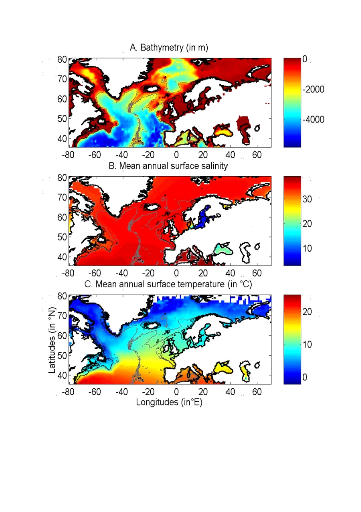
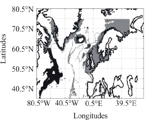
Figure II.1 : Spatial distribution of bathymetry (A), mean annual sea surface salinity (B) and mean annual sea surface temperature (C). Isobaths 200m (dark grey line) and 2000m (light grey line) are indicated. To assess the potential impact of changes in SST, data (1990-2100) from the Atmosphere-Ocean General Circulation Model (AO-GCM) ECHAM 4 (EC for European Centre and HAM for Hamburg; (Roeckner et al. 1996) were used; these data are projections of monthly skin temperature equivalent above the sea to SST (http://ipcc-ddc.cru.uea.ac.uk). Data used here are modelled data based on scenario A2 (concentration of carbon dioxide of 856 ppm by 2100) and B2 (concentration of carbon dioxide of 621 ppm by 2100) (Intergovernmental Panel on Climate Change 2007b). Scenario SRES (Special Report on Emissions Scenarios) A2 supposes an increase of CO2 similar to that currently observed. Scenarios SRES A2 and B2 reflect world populations of 15.1 and 10.4 billion people in 2100, respectively (Intergovernmental Panel on Climate Change 2007b). We also used data from the model HadCM3 (Hadley Centre Coupled Model, version 3) (Gordon et al. 2000). Both scenarios SRES A1B and B1 were used. Scenario A1B reflects a world of rapid economic growth, low population growth and rapid introduction of new and more efficient technology whereas scenario B1 reflects a world with rapid introduction of resource-efficient technologies (Intergovernmental Panel on Climate Change 2007b). Two non-SRES scenarios were also utilised: PICTL (i.e. experiments run with constant pre-industrial levels of greenhouse gasses) and COMMIT (i.e. idealised scenario in which the atmospheric burdens of long-lived greenhouse gasses are held fixed at the 2000 level). The model HadGEM1 (Hadley Centre Global Environmental Model, version 1) was also used with the non-SRES scenario 1PTO4x (1% to quadruple) in which greenhouse gasses increase from pre-industrial levels at rate of 1% per year until the concentration has quadrupled and become constant thereafter (Johns et al. 2006). This is the more pessimistic of all scenarios considered here. Therefore, a total of 7 scenarios (A2, B2, A1B, B1, PICTL, COMMIT and 1PTO4X) was used from 3 different AO-GCMs (ECHAM4, HadCM3, HadGEM1). The best estimate of temperature change is 0.6°C for COMMIT, 1.8 for Scenario B1, 2.4 for Scenario B2, 2.8 for Scenario A1B and 3.4 for Scenario A2 (Intergovernmental Panel on Climate Change 2007b). These forecasted SST datasets were used to examine how the probability of occurrence of cod varied as a function of (1) the intensity of warming and AO-GCMs and (2) identify regions susceptible to be the most influenced by the intensity of warming. All physical data were interpolated bilinearly on a spatial grid of 0.1° longitude x 0.1° latitude in a spatial domain ranging from 80.5°W to 70.5°E and from 35.5°N to 70.50°N (Fig. II.1). We used a high spatial resolution to decrease potential bias that could arise from the averaging of bathymetry data in a large geographical cell. The high resolution also enabled to have a better assessment of the probability of cod occurrence along coastline. While only one map of bathymetry and SSS (annual climatology) was generated, a grid for each year of the period 1960 to 2006 was built for SST. Therefore, the spatial distribution of cod varies according to the three abiotic parameters, while year-to-year changes were only a function of SST. ? Fish data Data of cod occurrence were taken from Fishbase ( http://www.fishbase.org; Froese & Pauly 2009). This represented a total of 52,630 data. Unfortunately, while high densities of data are present in the dataset on the western side of the North Atlantic this is not the case on the eastern side. Of the 52,630 data taken from Fishbase, only 9,638 data were located to the east of 30°W. Therefore, we completed the dataset from the knowledge of the spatial distribution of the species (ICES 2005a, Brander et al. 2006, Heath & Lough 2007, ICES 2007) (Fig. II.2). The data largely reflect the occurrence of cod 1 year (http://www.fishbase.org), although no distinction was made on age. Data therefore originated from scientific cruises, agencies, museums, university, nongovernmental organization, commercial catches, occasional fishermen and expert knowledge. The total number of data-points equalled 140,026 observations. For each observation of cod occurrence, information on sea surface temperature, bathymetry and sea surface salinity were added to each datapoint by interpolation of each environmental data from the datasets described above (see section on physical data). To compare results of our ecological niche model, we used probability data of cod occurrence obtained from the numerical procedure Aquamaps ( http://www.fishbase.org). This derives from the Relative Habitat Suitability (RES) model that was initially developed for mapping mammal species distribution (Kaschner et al. 2006) and has been adapted subsequently to map the probability of occurrence of all marine organisms. A total of 62160 data points were used to produce the probability map. Although no distinction was made on age the data reflect mainly the occurrence of cod = 1 year old ( http://www.fishbase.org).
Figure II.2 : Spatial distribution of observed (Fishbase data, 52,630 datapoints, in black) and inferred (104,642 datapoints, in grey) occurrence data point of the Atlantic cod (Gadus morhua Linneaus, 1758). Isobaths 200m (dark grey line) and 2000m (light grey line) are indicated. ? Description of the Non Parametric Probabilistic Ecological Niche model (NPPEN) The model is derived from a test recently applied to compare the ecological niche of two species (Beaugrand & Helaouët 2008). The analysis is based on Multiple Response Permutation Procedures (MRPP), a test first proposed by Mielke et al. (Mielke et al. 1981). MRPP has been applied in conjunction to Split Moving Window Boundary analysis to detect discontinuities in time series (Cornelius & Reynolds 1991). This method has also been used to identify abrupt ecosystem shifts (Beaugrand 2004, Beaugrand & Ibanez 2004). Mathematically, MRPP tests whether two groups of observations in a multivariate space are significantly separated. (Mielke et al. 1981) gave a full description of the test and Beaugrand & Helaouët (Beaugrand & Helaouët 2008) have recently illustrated an adaptation of the test to compare two ecological niches. The model we propose to assess the probability of cod occurrence (and its changes in space and time) is in fact a simplification of MRPP. Instead of comparing two groups of observations, our new analysis tests whether one observation belongs to a group of (reference) observations we call here the reference matrix. The reference matrix is represented by a matrix Xn,p with n the number of (reference) observations and p the number of variables. Each row of the matrix represents the environmental conditions where a species is detected. It is crucial that the reference matrix covers the entire niche of a species to give a reliable probability (Thuiller 2004); we check this point, which is often forgotten in this kind of exercise, by compiling histograms. The predictive matrix Ym,p encompasses m observations of the environment using p predictors. Each observation of Y, (environmental conditions) is then tested against X (range of conditions where the species was detected). The model is applied in 4 main steps: Step 1: homogenization of the reference matrix The density of cod occurrence reported in some databases (e.g. Fishbase) depends on fishing activities and it is clear that the density of data points is higher in fishing area. Although this suggests that the resource is more abundant in those regions, this is not completely true. This phenomenon can potentially influence the outcome of any ecological niche model. Another phenomenon that can influence the probability is the inaccurate reporting of occurrence since misreports can influence the probability. In an attempt to overcome these drawbacks, we created a virtual cube (i.e. three controlling factors) with intervals of sea surface temperature of 1°C between -2°C and 18°C, intervals of bathymetry of 20 m between 0 and 800 m and intervals of annual SSS of 2 between 0 and 40 and retained one data occurrence when more than one observation were detected in the crossed intervals of annual SST, bathymetry and annual SSS. This threshold was fixed to eliminate the impact of one single misreporting. The resolution could, at first sight, appear to be coarse. However, the practice of the ENM indicates that the probability remains similar, even at a lower resolution (see Fig. II.4), which depends on the size of the reference matrix. Here, the size was equal to 140,026 observations. This amount divided by 16,000 (20 SST intervals x 40 bathymetric intervals x 20 SSS intervals) = 8.75 observations per geographical cell. Such a calculation assumes obviously that observations are equally distributed, which was clearly not the case. A resolution of 0.1°C for SST, 1m for bathymetry and 0.1 unit of SSS would appear to be too sensitive as only 0.02 observations per crossed interval are expected if observations were randomly distributed. The determination of the threshold also depends on the uncertainties on the physical variables. Step 2: preparation of data A matrix called Zn+1,p is created for each observation of Y to be tested against X. For the first observation, the following matrix is constructed:
With xi,j, the observations in matrix X and yi,j, an observation of matrix Y. The building of matrix Z is repeated m times, corresponding to the m observations of Y. Step 3: calculation of the mean multivariate distance between the observation to be tested and the reference matrix MRPP was first proposed to be applied with an Euclidean distance, a squared Euclidean distance or a chord distance (Mielke et al. 1981). To first illustrate the technique, we use an Euclidean distance. Obviously, if variables do not have the same unit or dimension, such a distance should be avoided. The Euclidean distance is calculated as follows:
With z1,j the first observations for the jth variable originally the observation of the variable of matrix X, 1 = j = p; zi,j, the observation i of the variable j in matrix Z with 2 = i = n+1 and 1 = j = p. Then, the average observed distance åo is calculated as follows:
With n, the total number of Euclidean distances, equal to the number of observations in the training set X. Step 4: calculation of the probability that the observation belongs to the reference matrix The mean Euclidean distance is tested by replacing each observation of X by y in Z from row 2 to n+1. The number of maximum permutations is equal to n. After each permutation, the mean Euclidean distance ås is recalculated, with 1 = s = n. A probability p can be assessed by looking at the number of times a simulated mean Euclidean distance is found to be superior or equal to the observed mean Euclidean distance between the observation and the reference matrix X.
Where the probability p is the number of times the simulated mean Euclidean distance was found superior or equal to the observed mean distance. When p = 1, the observation has environmental conditions that represent the centre of the species niche. When p = 0, the observation has environmental conditions outside the species niche. It is essential to remind here that the niche and its borders have to be correctly assessed. Applying the procedure to each observation of Ym,p leads to a matrix Pm,1 of probability. It is important to have a large reference matrix so that the resolution of the probability is as high as possible. The resolution R of the probability is:
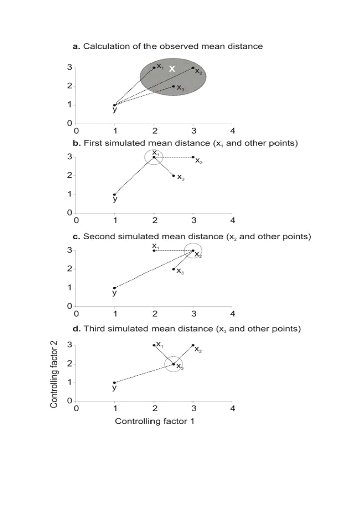
With n the number of reference observations in X. Ideally, R should be < 0.05. ? Simple example of application of the model using the Euclidean distance To illustrate the principle of the technique, we present a hypothetical case where the reference matrix X has n = 3 observations and p = 2 controlling factors while the predictive matrix Y has m = 1 observation (Fig. II.3). Calculations of the three Euclidean distances between y and the reference observations x give probability is therefore equal to 0. Observation y has environmental conditions not compatible with the species ecological niche inferred here from 2 variables. ? Selection of a better coefficient of distance for Step 2 Mielke et al. (Mielke et al. 1981) used mainly the Euclidean, squared Euclidean and chord distances. However, in the context of habitat modelling, the use of the Euclidean (squared or not) distance in step 2 is inappropriate in most (if not all) cases and the chord distance is often a better approach (Beaugrand & Helaouët 2008). The computation of the chord distance is achieved by normalizing each vector of Z to one prior to the calculation of the Euclidean distances; this is a special kind of scaling (Legendre & Legendre 1998). Each element of the vector is divided by its length, using the Pythagorean formula to ensure that each variable carries the same weight in the analysis. In our study, the normalization of elements of Zn+1,p (see (1)) would be:
Where x and y are as in (1). Here however, we prefer the use of the Mahalanobis generalised distance that is independent of the scales of the descriptors (as is the chord distance) but also takes into consideration the covariance (or the correlation) among descriptors (Ibañez 1981).
Figure II.3 : Principles of the calculation of the niche model that lead to probability of occurrence of a species. A. Hypothetical observations to be tested against a training set (X) composed of three observations in the space of two controlling factors. Three Euclidean distances are first calculated and then the average observed distance between the observation to be tested and the ones of the training set is assessed. B. Recalculation of the mean distance after permutation of the first observation (x1) of the training set by the observation to be tested. C. Recalculation of the mean distance after permutation of the second (x2) observation of the training set by the observation to be tested. D. Recalculation of the mean distance after permutation of the last observation (x3) of the training set X by the observation to be tested. All calculated Euclidean distances are indicated by a dashed line. The number of times the simulated mean distance is found inferior to the observed mean distance defined the probability to find the species in a region.
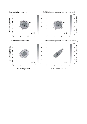
Figure II.4 : Fictive examples that show the better performance of the Mahalanobis generalised distance in comparison to the chord distance, justifying the choice of the distance coefficient in the ecological niche model NPPEN. First, the reference matrix is composed of 25 observations with two controlling factors. The correlation between the 2 controlling factors is null (A and B). A. Probabilities based on the chord distance (r = 0). B. Probabilities based on the Mahalanobis generalised distance (r = 0). Second, the reference matrix is composed of 13 observations with 2 parameters. The correlation between the two controlling factors is high (r = 0.82; C and D). C. Probabilities based on the chord distance (r = 0.82). D. Probabilities based on the Mahalanobis generalised distance (r = 0.82). Black circles denote the reference observations (reference matrix). High probabilities are located at the centre of the reference matrix, denoting the centre of the ecological niche (sensu Hutchinson) and probabilities <0.1 are situated outside (white colour). The Mahalanobis generalised distance has been frequently used recently in this context (e.g. Chalenge et al. 2008, Nogués-Bravo et al. 2008). Prior to the calculation of the distance, standardisation of Z is accomplished by the following transformation:
Where
With Rp,p the correlation matrix
of the standardized table Z* (mean 0 and variance
1), k1,p is the vector of the differences between
values of the p variables at ? Analyses Analysis 1 A comparison of the model based on a chord distance and the Mahalanobis generalised distance was performed using an example of 2 variables and in two cases: no correlation between the two variables (r=0, a training set of 25 observations) and a strong correlation between the two variables (r=0.82, a training set of 13 observations) (Fig. II.4). Analysis 2 The procedure of homogenization was illustrated by compiling histograms of each predictive variable (annual SST, annual SSS, bathymetry) for all geographical cells of the spatial domain covered by this study and for both the original and corrected training (or reference) set (Fig. II.5). Analysis 3 The model was then applied to project the spatial distribution of occurrence of Atlantic cod to enable the characterization of its ecological niche (realized niche) as a function of annual SST, annual SSS and bathymetry (Fig. II.6). The ecological niche was then projected in the spatial domain as a combined function of the three environmental parameters (observed annual SST, annual SSS and bathymetry) for the 1960s, the 1990s and the period 2000-2005 (Fig. II.7). Some projections of changes in the spatial distribution of cod occurrence, based on modelled SST (scenario A2 and B2; annual SSS and bathymetry), were provided for the 1990s (for comparison purpose), the 2050s and the 2090s (Fig. II.8). |
|


 (1)
(1) (2)
(2) (3)
(3) (4)
(4) (5)
(5) = 2.236,
  = 2.236 and
  =1.803 (Fig. II.3a). The average observed distance åo
is = 2.092. The simulated distances are ås1 = 1.589 (Fig.
II.3b), ås2 = 1.383 (Fig. II.3c) and ås3 =
1.140 (Fig. II.3d). The
=1.803 (Fig. II.3a). The average observed distance åo
is = 2.092. The simulated distances are ås1 = 1.589 (Fig.
II.3b), ås2 = 1.383 (Fig. II.3c) and ås3 =
1.140 (Fig. II.3d). The 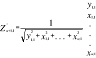 (6)
(6)
 (7)
(7) are observation i of the jth variables in Z,
  the average value of variable j and
  the standard deviation of variable j in Z. To calculate the Mahalanobis
generalized distance between each observation of the environment yi
(1 = i = m) and all observations of the training set xj (1 = j = n),
we used a particular form of the generalized distance, giving the distance
between any observation and the centroid of a unique group (Ibañez
1981):
the standard deviation of variable j in Z. To calculate the Mahalanobis
generalized distance between each observation of the environment yi
(1 = i = m) and all observations of the training set xj (1 = j = n),
we used a particular form of the generalized distance, giving the distance
between any observation and the centroid of a unique group (Ibañez
1981):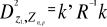 (8)
(8) of standardized matrix Z* and the mean
  of the p variables in the standardized matrix Z*. Therefore
in Step 3, the Euclidean distance was replaced by the use of the Mahalanobis
generalised distance.
of the p variables in the standardized matrix Z*. Therefore
in Step 3, the Euclidean distance was replaced by the use of the Mahalanobis
generalised distance.