4.5 GIS-Based Hydrological Model Development
4.5.1 Introduction
In order to compute the water resource availability and to
simulate the spatial and temporal distribution of water balances over the Congo
River Basin (CRB), a GIS-based hydrological model, namely HATWAB (Hybrid
Atmospheric and Terrestrial Water Balance) was developed and parameterized for
the Congo basin (Figures 27 and 28), based on the initial model of Alemaw
(2006). Initially, a GIS based hydrological model (Alemaw, 1999) was developed
to computer the spatial and temporal distribution of water balance in southern
Africa reion. This model was modified and used for the same region (Alemaw and
Chaoka, 2003) and for the Limpopo basin (Alemaw, 2006). The approach of this
model is based on the parametersization of input data, viz monthly
temperature, precipitation, land-cover/use, soil texture and rooting depth and
the Digital Elevation Model, to compute temporal and spatial variability of
water budgets at geo-referenced grids cells covering the Congo basin.
The atmospheric component of the water balance model computes
the Integrated Vertical Moisture Convergence (C) based on the precipitation and
evaporation, while its terrestrial component estimates Actual Soil Moisture
(SM), Actual Evapotranspiration (AET), and Runoff (TRO). Surface abstractions
components in term of overland runoff (DRO) and interception are also
accounted. The model estimates the uncertainties on water balance parameters
and as well as the imbalances.
A separate component of the model consists of a DEM
hydrological processing. This component extracts watershed and streams network
(Figure 12), compute their hydrogeomorphometric parametes which characterise
the topography, topology and hydrography of the river basin.
The Spatial and temporal distributed water balance model
requires various types of data from different sources (Melesse et al, 2006)
like Remotely-sensed datasets (NDVI images, DEM), meteorological datasets
(precipitation, air temperature, wind speed, sunshine hours, etc), hydrologic
(river discharge), hydrologic soil maps and other GIS layers ( watershed
boundaries and properties, streams topology, etc) in raster,vector and tabular
formats. Their collection and preparation will be presented in section 5.4.
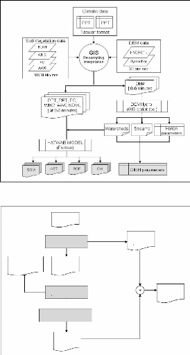
Figure 27 General terrestrial Water Balance model
structure
RAINFALL
(PPT)
Surface process
EPPT = PTT -DRO
EFFECTIVE
RAINFALL
(EPPT)
DIRECT RUNOFF (DRO)
Soil storage
(FC, WP, AWC...)
Excess =
EPPT- DRO - AET-? SM
RUNOFF
STORAGE
(RO)
TOTAL
RU NO
FF
(GRID)
ACTUAL
EAVPO-
TRANSPIRATION
Figure 28 Rainfall-Runoff simulation model for a single
grid cell
4.5.2 Water Balance Model development
procedure
The water balance model development comprises the following
steps:
(i) Vertical Integrated Moisture
convergence:
The Vertical Integrated moisture convergence (C) is a component
of the atmospheric water balance and will be computed based on rainfall and
Evapotranspiration data.
(ii) Rainfall-Runoff Development
At this stage, components derived from previous steps will be
used to generate monthly water balance compounds as shown in Figures 27 and 28:
Runoff (TRO), Actual Evapotranspiration (AET), Soil Moisture (SM) and
Percolation (P). The Thornthwaite and Mather (1957) method, slightly modified,
generate a monthly water balance for each grid-pixel as well as for the whole
Congo River Watershed.
(iii)DEM-Hydro processing: Watershed and Streams
delineation
Watershed and sub-watershed boundary maps are required to
delineate the specific area where the soil-water balance model will be applied.
In other words, the model will account for the water balance for the grid cells
falling in the watershed limits. These files, namely `MASKS', are extracted
during the DEM processing.
The DEM-Hydro Processing were developed in section 4 in order
to derive Geomorphometric properties of the catchments and stream network like
flow direction, flow accumulation, catchment, drainage network, overland flow,
masking files, and other hydrologic data using GIS packages (viz ILWIS 4.3 and
ESRI ArcMap 9.2 versions). The Horton statistic parameters were used for
discriminating and characterizing the extracted watershed and streams from the
DEM.
4.5.3 Water Balance Model Development
Supposing the principle of continuity in hydrologic system,
Chow (1998) assumes that the time rate change of storage is equal to the
difference between the input and the output in of the hydrologic model
(equation 26).
where, St is the time-variant storage in a grid cell,
It , the summation of input coming into the cell from upstream cells
and the runoff generated in the cell, and Ot , the outflow from the
cell which is calculated by various methods, e.g. the linear reservoir
method.
4.5.3.1 Atmospheric water balance
The atmospheric component of the water balance model is expressed
as
dWPEC
dt = - + + (27)
C=-?×Q (28)
Where dW/dt is the amospheric storage change, C is the
vertical integrated moisture converence (LT-1) and was expressed as
a function of the water vapour flux (Q) in Equation (28).
? × Q is the divergence or net outflow of water
vapor across the sides of the atmospheric column, Q is the vapor flux, E is
evaporation, and P is precipitation.
The quantity W is also referred to as the precipitable water
and may be expressed in units of mass per unit surface area [M L-2]
or converted to an equivalent depth of liquid water [L] by dividing by the
density of liquid water (1000 kg m-3).
The divergence Q mesures the difference between inflow and
outflow to a region; a positive divergence means that outflow is greater than
inflow, and a negative divergence (or convergence) means that inflow is greater
than outflow. The units of divergence are [M L-2 T-1] but
may also be expressed as depth of water per time [L T-1].
In mean water balance computation like the HATWAB model which
is monthly water balance model, the atmospheric storage change is often assumed
to be negligible (Reed et al, 1998 and Marengo, 2005); thus equation (28) is
reduced to

P-E=C or P-E=-?Q
(29)
|
|
|
From Equation (30), it is seen that if the divergence
(?Q
|
) in a region is positive, then
|
evaporation is greater than precipitation (P-E < 0), while a
negative divergence or "convergence" indicates that precipitation is greater
than evaporation (P-E > 0).
4.5.3.2 Terrestrial water balance
At monthly time scale a terrestrial water balance model is
written as
ds P E R
dt = - - (30)
Where S is soil moisture storage (L); P is
precipitation (LT-1); E, actual Evapotranspiration
((LT-1); and R, the observed runoff (LT-1).
Linearising Equation (30), the terrestrial water balance has the
following form
SM1 = SM t - 1 + P
t -E t - R t (31)
Where t is the time period, which is a single month is this
model, P is precipitation, E is the Evapotranspiration, and RO is the
runoff.
Once the initial soil moisture (St-1) and the actual
soil moisture (St) are determined, the monthly Actual Evapotranspiration Et and
the Runoff Rt can be calculated.
4.5.3.3 Imbalance estimation
Combining Equations (30) and (31), the vertical integrated
moisture convergence (C) is computed as follows
dS
C R
- = (32)
dt
In a steady state P AET =R. Changes in storage could
however lead to P E being different from R. These could also be due to
certain errors in representing rainfall within the Congo River Basin. These
lead to the expression of an imbalance equation
C ds dt R
- ( / + )
Imb = (33)
R
The imbalance in Imb is calculated using the
following formula:
C ds dt
/
Imb (34)
= - + 1
R R
Contrary to the formulation adopted in this study based on
(34), Marengo (2005) assumes that dS/dt is negligible for monthly time
scales and applied it in the Amazon basin, which reported unaccounted residuals
in his water budgets. Whereas in the proposed model in this study, the soil
moisture variation dS/dt is varying from season to season as a
function of the prevailing PET and PPT at a given location
according to Equation (30), in which the imbalance should also cater for this
variability according to Equation (34). One of the contributions of this study
is that, once the imbalance (Equation 34) is kept to a minimum in the water
balance computation at each grid, then the simulated variables and water
balances, PPT, ET, RO, RO/PPT,
ET-PPT, ET/PET, S and C can then be used to
investigate the seasonal and temporal variability of water budget of the Congo
basin.
The amount of precipitation and potential evapotranspiration
determines soil moisture availability, which in turn is controlled by the water
holding capacity of the soils. Solution of the mass balance equation will be
solved for E, R and S (section 4.5.3.4).
4.5.3.4 Rainfall-Actual Evapotranspiration-Soil
moisture-Runoff modelling 4.5.3.4.1 Effective Precipitation (EPPT) and
overland runoff (Direct runoff DRO)
One of the main inputs required in the proposed water balance
model is the effective precipitation (EPPT). At a monthly time scale, the
effective precipitation is calculated as per the formula of the USDA soil
conservation available from FAO (1990) as follows:
125 0.2
- PPR
EPPT PPT for PPT mm
= ( ) 250
< (35)
125
EPPT = 125 + 0.1 PPT forPPT=250 mm
(36)
Where EPPT is effective precipitation and PPT
is the total precipitation
The direct runoff (DRO) is the difference between the
precipitation (PPT) and the Effective precipitation (EPPT).
4.5.3.4.2 Soil moisture estimation
(SM)
Soil moisture is determined from the interaction between
effective PPT and PET. During wet months (when effective PPT in excess of PET),
soil moisture can increase up to a maximum of field capacity determined by soil
texture and rooting depth.
dt
dSM = EPPT - PET when EPPT > PET and SM < FC
(37)
dt
dSM = 0 when SM = FC (38)
dSM ( - )
dt
= a SM PET EPPT when EPPT < PET (39)
Where, FC is the soil moisture at field capacity of the soil
millimetres, PPT is precipitation in mm/month; PET is potential
evapo-transpiration in mm/month.
During the dry periods where the EPPT < PET, the soil
becomes increasingly dry, soil moisture becomes a function of potential soil
loss. Thus, different authors assumed different relationship to find the soil
moisture during the dry periods (Thornthwaite, 1948; Vorosmarty et
al., 1989).
For a particular soil, there is a linear relationship between
Log (SM) and Ó(EPPT-PPT) summed from the start of the dry season to the
current month. Thus, to calculate the rate of change of soil moisture (ÄS)
through the dry season, the soil moisture is directly estimated from the
empirical relation suggested by Vorosmarty et al. (1989). To calculate
ÄSM/dt through Equation (40) for intermediate field capacities, the HATWAB
defines a slope a to the retention function as:
a = ln(FC)/(1.1282 FC)1 . 2756 (40)
where the numerator represents soil moisture (millimetres) with
no net drying. The
denominator is the accumulated potential water loss or
APWL ( ? [PET - PPT ]) in mm
at SM=1 mm. With a determined, the model can
calculate dSM/dt as a function of soil dryness and update SM. Figure 29 shows
the relationship between soil moisture and the Evapotranspiration. Between the
plant wilting point and the root zone Field Capacity, Evapotranspiration
increases with the soil moisture.
Calculations commence at the end of the wet season when it is
assumed the soil is at the field capacity. Soil water stocks are then depleted
during the dry season in accordance with the moisture retention function. For
each wet month, soil moisture is determined by incrementing antecedent values
by the excess of the available water over PET. This recharge may or may not be
sufficient to bring the soil to field capacity at the end of subsequent wet
season.
ETa/ETp


1

WP FC=WH
Figure 29 Functional relationship between soil
moisture and Evapotranspiration (ETa is the actual Evapotranspiration, ETp is
the potential Evapotranspiration, SM is the soil moisture, FC is the field
capacity and WP, the Wilting point
Analysis of the ratio PPT/PET at the various grids in Central
Africa has shown that the region can not be represented by one homogeneous
climatic zone, rather it is a combination of climate influenced by the
diversified hydro-climatic conditions in the region. In this analysis, it has
been observed that the long-term monthly rainfall distribution varies greatly
in the region.
It is assumed that the ratio PPT/PET could be a good indicator
of the seasonal distribution of monthly rainfall, and accordingly the wet
season ends when the ratio PPT/PET just starts to fall below unity. In line
with this, therefore, the soil moisture can be assumed to be at its field
capacity. Consequently, HATWAB fixes a starting month of any grid across the
region according to the aforementioned criterion. The solution of the basic
mass balance equation for the subsequent months can determined once the initial
soil moisture state is obtained.
4.5.3.4.3 Actual Evapotranspiration
(AET)
Once the actual soil moisture is determined, the corresponding
actual evapotranspiration (AET) is calculated for the month. Following the
Thornthwaite and Mather (1957) approach, AET is set equal to PET in wet months,
when EPPT > PET. During this time it is assumed that EPPT is in sufficient
abundance to satisfy all the potential water demands of the resident
vegetation. During dry season when EPPT < PET, the monthly average AET is
modified down wards from its potential value as shown below.
AET = PET when EPPT > PET (41)
dSM
AET = EPPT - when EPPT < PET (42)
dt
where the soil moisture drops below the wilting point, the AET is
equal to the EPPT but if there is no EPPT at all time, AET becomes zero.
4.5.3.4.4 Total runoff (TRO) generated at a grid
spatial scale
Most of the water does not leave the basin as soon as it
becomes available as surplus. The
portion that constitutes overland
flow is assumed to flow out of the watershed within the
month it occurs but the portion that infiltrates may take a
number of months to move slowly through upper layer of the soil column to
emerge in the surface water courses as base flow.
The lag or delay factor depends not only the size of the basin
but also on the vegetation cover and the soil type, degree of slope,
characteristics of the soil layers, etc. Thornthwaite suggested that 50 % of
the water surplus could be assumed to runoff each
month from large basins with the remainder being held over and
added to the surplus of the next month. This factor is set according to
Thornthwaite & Mather (1957) which is equal to 0.5.
RO = (D + (EPPT - PET) when SM = FC EPPT > PET
0 . 5 * ) &(43)
RO = 0.5 * D when SM < FC EPPT < PET
& (44)
Where, RO is rainfall-driven runoff or surplus runoff (mm/month)
and D is the amount of detention storage in millimeters that is assumed to
leave each grid cell next month.
4.5.4 Data sets and software
This study requires a set of hydro- meteorological variables
(rainfall, evapotranspiration, and wind speed), topographic data or Digital
Elevation Model (DEM) data set, landcover/use variables, vegetation, soil
data.
4.5.4.1 GIS and geo-referencing procedure
The Congo River basin has a sub-continental extension covering
8 countries in Central Africa region. It is extended between 150S to
100N and 100E - 35 0E. Originally, the area of
study has a spatial resolution of 30x30 minutes but for a better resolution and
accuracy of the results a 6 minutes (averaged to 12km at the equator) was
adopted and forced by the computational techniques.
The Kriging method (Krige, 1966; Stein, 1998, Surfer v.8) was
used to interpolate and fill the missing value, harmonizing different data sets
to a spatial resolution of 6 minutes for a single grid cell, corresponding to
62500 square grids (250 rows and 250 columns).
4.5.4.2 Meteorological data sets
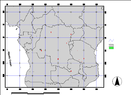
Free meteorological data for 3262 global climatic stations are
available at FAO-UNESCO /CLIMWAT, with a record time of 30 years (1961 -1990)
at a monthly scale; where 145 climatologic stations covering the study area
(Figure 29 and Appandix 1) were extracted to compile the meteorologic database
for the model. These climatologic data sets include monthly averages of maximum
and minimum of temperatures, mean relative humidity, wind speed, sunshine
hours, radiation data as well as rainfall and Reference Crop Evapotranspiration
(ETo) calculated with the Penman-Monteith method (Allen et al, 1998). Below,
Figures 31 and 32 show the Rainfall and Potenital Evapotranspiration
distribution in the basin, respectively.
700 0 700 1400 Kilometers
Enugu
%
Kano
Libreville
Pointe Noire
%
Douala
%
%
Malabo
%
Port Gentil
%
Benguela
$
Luanda
Yaounde
%
Brazzaville
$
$
$
%
$
$$
M $
atadi $ $
%
$
$
%
$
$
$
$
% %
Huambo
%
Maiduguri
$ $
$
$
$
$
$ % %
%
$
$
$
$
Kinsha
$
$
$
$
$
$
Mbandaka
$
$
$
$
$
$
$
Kahemba
%
Bangui
$ %
$
$
$
%
$
$
$
$
$
$
$
$
$
$
$
$
$
$
$
$
%
$
$
$
$
$
Kananga $ $ $
$$
$ $
$
$
$
$
$ Kisangani
$ $ %
Lumumbashi
$ $
Livingstone
$ $
%
$
$
$
$
$
$
$
$
$
$
$ Kigoma
$
%
$
$
$
$
Lusaka
$$ %
$
$
$
$
$ $
%
$
$
$
$ $ $
$
$ Kigali
%
$
$
$
$
%Bujumbura
Harare
$
$
$
%
Kampala
%
$
$ $
$
$
$
$
$ Lilongwe
%
$
$
Dodoma
$
$
$
$
Beira
$
Dar es Salaam
Nairobi
%
Adis Abeba
Mocambique
%
%
Mtwara
%
%
%
Mombas
%
Djib
An
$ Stations zxy.txt
% Cities.shp
Afrbord.shp
Afpolit.shp
Latlong.shp
Figure 30: Distribution of Climatic stations in the study
area. The study area covers more than 145 stations

10
-10
-15
-5
5
0
|
Annual Rainfall
|
|
|
|
|
mm/year
2100 1900 1700 1500 1300 1100 900 700
|
|
|
|
|
|
|
|
|
|
|
|
|
|
|
|
|
|
|
|
|
|
Annual Effective
|
Rainfall
|
|
|
|
mm/year
1600 1500 1400 1300 1200 1100 1000 900 800 700 600
|
|
|
|
|
|
|
|
|
|
|
|
|
|
|
|
|
|
|
|
|
10 5 0 -5 -10 -15
10 15 20 25 30 35 10 15 20 25 30 35
10 15 20 25 30 35
10 15 20 25 30 35
Figure 31 Rainfall averaged (1961-190) data from 145
stations. 1. Rainfall, 2. Effective Rainfall
10 5 0 -5 -10 -15
Annual Potential
|
Evapotranspiration
|
|
|
mm/year 1800 1500 1400 1300 1200 1100 1000
|
|
|
|
|
|
|
|
|
|
|
|
|
|
|
|
|
|
|
|
|
|
|
10 15 20 25 30 35
Figure 32 Mean Annual Potential Evapotranspiration
(1961-1990) map
4.5.4.3 Discharge data
There is a lack of discharge data in the Congo Basin although
there is Rainfall gages and data since 1958. The availability of recharge data
is limited to a few numbers of rivers gauges. At the basin final outlet,
discharge has been amounted to an average of 45000 m3/sec (Asante,
2000).
Discharge data indicate a series of four distinct phases in
the Congo and the Oubangui since the beginning of the 20th century.
During the 1 960s they increased, overtaking their average over a century. The
Congo discharge then fell, returning in 1970 to what had been the normal level,
whereas the Oubangui entered a drought phase. This trend accentuated from 1980
and, until 1996, the Congo discharge weakened by 10% (37 400 m3/s in 1992
compared with an average of 40 600 m3 /s over that period as a whole), which
was the most dramatic decrease of the century. This fall is much stronger in
the Oubangui (- 29%), yet negligible (- 0.2 %) in the Kouyou sub-basin.
Overall, whereas discharge decrease in the Congo Basin is between two and four
times the drop in rainfall (IRD, 2002) Table 14 summarises the Congo River
discharge (1903 -1983) at Kinshasa station.
4.5.4.4 Digital Elevation Model (DEM) and Mask
files
The topographic properties of the area were derived from a DEM
raster data namely HYDRO1k. The HYDRO1k is a geographic database developed at
the U.S. Geological Survey's EROS Data Centre to provide comprehensive and
consistent global coverage of topographically derived data sets, including
streams, drainage basins and ancillary layers derived from the USGS' 30
arc-second digital elevation model of the world (GTOPO30).
The HYDRO1k has the advantage of being hydrologically
corrected for calculation of derived hydrologic parameters such flow direction,
flow accumulation, slope (Asmamaw, 2003); and it is freely available at a
standard suite of geo-referenced data sets with a spatial resolution of 1
kilometre, adapted for a large scale water balance model. Figures
14 and 21 show the DEM of the study area and the polygon map of
the entire CRB and sub-watersheds `Mask files».
4.5.4.5 NDVI and vegetation database
The monthly NDVI images for each basin were acquired from the
Global Land Cover Characteristics database. Satellite data have been used
extensively for mapping the land use and for monitoring the seasonal change of
vegetation of river basins (Nemani & Running, 1989).
The Normalized Difference Vegetation Index (NDVI) is commonly
applied to derive the leaf area index (LAI) from channels 1 and 2 of
NOAA-AVHRR data at 1 -km2 resolutions. Monthly twelve NDVI images,
expressed in percentage, for 1987 are acquired from USGS web pages. Based on
NDVI values the LAI for different land use groups can be estimated by empirical
formulae. Table 13 presents rooting depth assigned for various soil textures
and SCS soil groupings
Table 13 Rooting depth assigned for various soil textures
and SCS soil groupings
|
Veg.
Group
|
NDVI
|
Assigned Root Depth (M) For Different Soil Types
|
|
Sand
|
Sandy Loam
|
Silty
Loam
|
Clay Loam
|
Clay
|
Lithosol
|
|
VEG2
|
>50%
|
2.5
|
2.0
|
2.0
|
1.6
|
1.2
|
0.1
|
|
VEG1
|
=50%
|
1.0
|
1.0
|
1.3
|
1.0
|
0.7
|
0.1
|
|
SCS soil group (Singh, 1992)
|
A
|
B
|
D
|
C
|
C
|
B
|
4.5.4.6 Soil properties
A global Soil map at 10x10 minutes resolution is freely
available at FAO/UNESO database (FAO, 1984). This map is used to extract the
submap of the study area and later re-sampled to a spatial resolution of 6x6
minutes so that it can overlay onto the model.
Since the Soil Water available to plants depends on soil water
content, soil texture (Figure 33), and consequently, the rooting depth of
vegetations, the 133 agronomic groups of FAO agronomical soil map were
therefore used to derive and reclassify textural soil classes which are
required as input data for the model. For this matter a FORTRAN algorithm was
developed and 6 hydrological textural classes of soil (Table 14 and 15) were
identified in the study area.
Table 14 Soil texture distribution in the Congo River
basin
|
Class ID
|
1
|
2
|
3
|
4
|
5
|
6
|
0
|
Total
|
|
Soil type
|
Sand
|
Sandy Loam
|
Silty Loam
|
Clay loam
|
Clay
|
Lithosol
|
Water body
|
|
No grids
|
4847
|
0
|
58
|
21867
|
989
|
2374
|
513
|
30640
|
|
% gris
|
15.8
|
0
|
0.2
|
71.3
|
3.2
|
7.7
|
1.7
|
100
|
The reclassified textural soil and vegetation maps are used to
derive the soil retention parameters such as Field Capacity (FC), Wilting Point
(WP) which determine the soil moisture capacity known as Available Water
Content (AWC) for each soil group.
Based on field measurements, Saxton et al. (1986)
have developed a technique to estimate the matrix potential of different soils
by using multiple regression techniques. Therefore, at a matrix potential
equivalent to field capacity (33 KPa) and wilting point (1500 KPa) for a unit
meter depth of soil, approximate values of FC and WP for the various soil
textures have been extracted (see Table 15). Accordingly, the FC and WP values
as per the rooting depth are then derived for the whole region as summarised in
Table (15). Available water content (AWC) of a soil of given texture is defined
as the difference between the field capacity and wilting point.
The depth of soil water which can be used by the crop, the
Total Available Water (AWC), depending on the root depth of the crop and on the
soil moisture holding properties of the soil (Eilers et al, 2007), Equations
(45, 46) bellow shows the relationship between these soil parameters:
AWC = (UFC-UWP)R (45)
|
With
|
FC UFC R
= ×
WP UWP R
= ×
|
(46)
|
Where AWC is the available water content per root depth;
FC and WP are the field capacity and wilting point,
respectively; R is the current depth of the roots; UFC and
UWP are the field capacity and the wilting point per unit volume of
the soil, respectively.
Figures 33-36 show the generalised relationship between the
soils parameters, the Textural soil groups, the Field capacity map, the Wilting
Point map and the Available water content map, respectively.
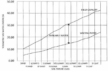
Figure 33 Available soil water vs. soil texture
showing estimates of field capacity, permanent wilting point and Available
water content. S-Sand, SI-Silt, CL-Clay, F-Fine, VF-Very Fine, L-Loamy (after
Levy et al, online)
Table 15 Relationship linking vegetation class, soil
texture, rooting depth and moisture capacities of various soil groups in
Central Africa (Source: Alemaw and Chaoka, 2003)
|
Sand Sandy Loam Silt Loam Clay Loam Clay Lithosol
|
|
Veg. Group
|
The Root depth (m)
|
|
GRP1
|
2.5
|
2.0
|
2.0
|
1.6
|
1.2
|
0.1
|
|
GRP2
|
1.0
|
1.0
|
1.3
|
1.0
|
0.7
|
0.1
|
|
2.3.2.1.1.1.1.1.1 FC and AWC of soils as % of total volume
of soils / m
|
|
% (FC)/m %(AWC)/m
|
14.1
6.3
|
20.0
9.1
|
27.3
13.2
|
35.2
35.8
|
48.5
35.8
|
27.3
13.2
|
|
2.3.2.1.1.1.2 Field Capacity and AWC per root depth of the
plant
|
|
GRP1 (FC)
(AWC)
|
353
196
|
400
218
|
546
282
|
563
243
|
582
153
|
27
14
|
|
GRP2 (FC)
(AWC)
|
141
78
|
200
109
|
355
183
|
352
152
|
339
89
|
27
14
|
-10
-15
10 15 20 25 30 35
10
-5
5
0
|
Textural Soil Types map
|
|
|
|
Soul types
6 Luthosol 5 Clay
4
|
|
|
|
|
|
|
|
|
Clay loam
3 SultLoam 2Sandy Loam 1 Sand
|
|
|
|
|
|
0 Water body
|
|
|
|
|
|
|
|
|
|
|
|
Figure 34 Hydrological Soil types over the
basin
10 5 0 -5 -10 -15
|
Soil Fiel Capacity in the root zone
|
|
|
mm/root depth
|
|
|
|
|
0
|
550 500 450 400 350 300 250 200 150 100 50
|
|
|
|
|
|
|
|
|
|
|
|
|
|
|
|
|
|
|
|
|
|
10 15 20 25 30 35
Figure 35 Soil Field Capacity in the root
zone.
10 5 0 -5 -10 -15
|
Soil Available Water Content
|
|
|
mm/root depth
|
|
|
|
|
0
|
240 220 200 180 160 140 120 100 80
60
40
20
|
|
|
|
|
|
|
|
|
|
|
|
|
|
|
|
|
|
|
|
|
|
10 15 20 25 30 35
Figure 36 Hydrological Soil types over the
basin
4.5.4.7 Software resources
The packages used in this research are FORTRAN Power Station,
ILWIS 3.4, ArcGIS 9.2, ArcViewGIS 3.3, Canvas7, Surfer v8.0 and CorelDraw v12,
and Microsoft Excel packages.
| 

