CHAPTER THREE
3.0 LITERATURE REVIEW
3.1 Hydrological models
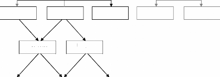
Hydrological model have been largely detailed and classified
(Figure 1) based on multiple parameters such as the model input data sets
types, and the physical characteristic of the model among others. However,
Hydrological models have, traditionally, been modelled as physically-based or
conceptual depending on the complexity and extent of completeness of the
structure of the model (Beven, 1989; Refsgaard et al., 1989;
Bergstrom, 1990; Refsgaard, 1996, 1998).
Hydrological
Models
|
|
|
|
|
|
|
|
|
|
|
Deterministic
|
|
|
|
Stochastic
|
|
|
|
|
|
|
|
|
|
|
|
|
|
|
|
|
|
|
|
|
|
Grid based
|
|
Subwatershed
|
|
No Distribution
|
|
|
|
|
Figure 11 Hydrological Model Classification
Probabilistic
Time Series
Physical
Based
Distributed
Conceptual
Lumped
Empirical
In physically-based water balance models, all the physical
phenomena like precipitation, evapotranspiration, ground water inflow, ground
water outflow and storage need to be quantified and modelled. Models are
further classified into lumped or distributed, based on basin terrain
(Bergstrom and Graham, 1998). In lumped models, spatial variability in
hydrologic parameters or meteorological related data are not accounted for,
meaning that they are averaged or assumed uniform over the system, whereas, in
distributed models spatial variability is explicitly accounted for by assuming
uniformity over smaller modelling units by sub dividing the bigger system based
on physical properties. In most of the distributed hydrologic models, these
units are delineated by combining climatic components, topography, soil
properties, land use properties and other pertinent properties. Distributed
models are especially useful, for example, when impacts of land use change are
to be studied or for analyzing spatially varying flood responses (Koka,
2004). The Lumped models are easy to implement, but do not
account for terrain variability whereas Spatially-distributed models require
sophisticated tools to implement, and account for terrain variability
(Oliveira, 2002).
A statistical model derives an empirical relationship between
precipitation, infiltration, flow and any other parameters that are included in
the model. The relationship is derived based on observed data for all the
dependent and independent parameters in the model. The best relationship is
identified using suitable statistical parameters (Sukheswalla, 2003).
Large scale modeling of streamflow can be done efficiently
using simple models (Becker and Braun, 1999; and Wolock and McCabe, 1999).
Distributed models require high resolutions for efficient modeling like the
MIKE SHE model (Ewen et al., 1999) and the TOPMODEL (Beven et
al., 1994). However, for large scales such high resolution is not always
available. Also, distributed models are generally not practical and efficient
for large-scale modelling (Becker and Braun., 1999), while statistical
lumped models that fulfil large scale modelling requirements of resolution and
computation time are better (Becker and Pfützner, 1987).
Using the cell-to-cell model, a watershed can be represented
as a single cell, a cascade of n equal cells, or a network of n equal cells
(Singh, 1989). The storage in the cells is calculated as given below:
(1)
dS= -
dt
t I O
t t
where, St is the time-variant storage in a
grid cell,
It is the summation of input coming into the
cell from
upstream cells and the runoff generated in the cell, and
Qt is the outflow from the cell which is
calculated by
various methods, e.g. the linear reservoir method.
Equation (1) is a generalized water balance model which can be
applied in different situations: atmospheric, surface, soil-water, groundwater
models. The types of input variables are defined by the researcher according to
the problem. Several books, papers ad reports describing the application of
equation (1) are available, viz Thornthwaite and Mather (1957), Chow
et al (1988), Reed et al (1997) and Rasmusson (1997).
| 

