4. EMPIRICAL RESULTS
Fig.1
![]()
Fig.1
|
Portf Mean
|
Portf Risk
|
VaR
|
CVaR
|
|
M-V
|
0.0024
|
0.0171
|
0.0242
|
0.0372
|
|
MCVaR
|
0.00208
|
0.02274
|
0.0285
|
0.043
|
|
BL Cov
|
0.0032
|
0.0214
|
0.0000
|
0.0000
|
|
BL CAPM
|
0.0034
|
0.0221
|
|
|
In this empirical section we consider the weekly return data
on the JSE-ALSI from early February 2003 till late September 2010. The market
capitalization weights on the efficient portfolio are dominant of 24.9% on the
USD/ZAR exchange rate following by Chemical Index and there is no weight
allocated to Life insurance Index. The mean conditional variance is giving the
following figures through the risk budgets; the highest shares are in chemical,
technology and beverage by respectively 22.7%, 22.6% and 20.1%. The life
insurance stills the only stock which doesn't have any allocation.
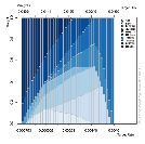
The fig.1 tells us that at a lowest risk with almost all the
weight will be allocated to USDZAR and some negative return on the USDZAR and
Technology Index. It's telling us also that at optimal point we have to
combine an important weight of the USDZAR with a target return of 0.000662 and
risk profile of 0.0111, following by Technology Index and almost a close weight
between the Bank Index and the Chemical. The highest level of risk will be
achieved with a target return of 0.0049 and Telecom will have the entire
maximum weight allocated.
The prior of the beverage index is very low to his posterior
while telecom has a high prior than the posterior. The highest weight is found
on the technology index where the prior and the posterior are almost closer to
0.8.
On fig.2 we have a highest portfolio mean on a Bayesian CAPM
which is the higher expected return and the lowest risk of the portfolio is
assigned to the Mean-Variance method. The highest expected value which can be
loosed and the highest expected value plus all negative losses is given by the
mean conditional value at risk method.
5. CONCLUSION
Traditional mean-variance portfolio optimization assumes that
it is extremely difficult to estimate expected returns precisely. In practice,
portfolios that ignore estimation error have very poor properties: the
portfolio weights have extreme values that fluctuate dramatically over time and
deliver very low Sharpe ratios over time. The Bayesian approach allows a
Bayesian investor to include a certain degree of belief in a portfolio
selection model. In this paper, we have shown how to allow
for the possibility of multiple priors about the estimated expected returns and
the underlying market return model. And, in addition to the standard
optimization of the mean-variance objective function over the choice of
weights, one also will provide the lowest value at risk and the conditional
value at risk. This study uses theoretically motivated prior and posterior
information about expected returns in portfolio selection. From an estimation
perspective, the focus on expected returns could be helpful since it is well
known that means are in general estimated with much less precision than
covariance. Nevertheless, using prior information to impose some structure on
the Black Litterman covariance matrix could potentially also be beneficial,
especially for a large number of stocks.
Reference
1. Polson, N. G., and Tew, B. V., 2000. Bayesian
portfolio selection: An empirical analysis of the S&P 500 index
1970-1996. Journal of Business & Economic Statistics,
18(2)
2. J.M MWAMBA, Slides of Bayesian asset pricing,
MCom Financial Economics, 2010
| 

