Modélisation des indices de prix sectoriels au Benin

CONCLUSION

En définitive, nos analyses ont porté dans un premier temps, sur la description de l'évolution des séries, ensuite sur l'étude de leur saisonnalité et leur stationnarité. Enfin, nous avons procédé à une modélisation ARIMA des séries de l'IHPC et à l'analyse des chocs.

De ce travail, il ressort que :

- toutes les séries sont non saisonnières ;

- des douze séries, seules les fonctions deux, cinq, onze et douze sont stationnaires en différence première ; toutes les autres sont stationnaires en niveau.

- la série FCT1 est un processus ARMA(6,7) ; les séries D(FCT2), FCT7, D(FCT11) sont des processus ARMA(2,12) ; les séries FCT3 et FCT4 sont des processus ARMA(4, 12) ; les séries D(FCT5), FCT8 sont respectivement des MA(12) et MA(13) ; la série FCT6 est un processus ARMA(2, 13) ; la série FCT9 est un processus ARMA(6, 10) enfin, les séries FCT10 et D(FCT12) sont des processus ARMA(1,12).

- un choc sur l'une des douze fonctions affecte les autres fonctions puis l'indice global des prix.

Plusieurs extensions de ce travail sont envisageables. En effet, cette modélisation des indices de prix sectoriels pourrait, par exemple, être complétée par des prévisions afin de permettre aux décideurs de mieux mener les politiques anti-inflationnistes.

BIBLIOGRAPHIE

· BEFFY P., MONFORT B. et al, 2003 << L'apport d'un modèle macroéconométrique pour l' analyse conjoncturelle >>, Insee.

· BOURBONNAIS R. ; TERRAZA M. ,1998 - << Analyse des séries temporelles en économie >>, Presses universitaires de France, Paris.

· BOURBONNAIS (R.), 2000, «Econométrie», ^3ième édition. Paris, Dunod.

· DOE L. et DIARISSO S., 1996, << Une analyse empirique de l'inflation en Côte d'Ivoire >> in Notes d'Information et Statistiques N° 465- Août/Décembre 1996. Dakar, BCEAO.

· DOSSOU A., 2000, << Guide pratique de l'économétrie des séries temporelles >>, Dakar, BCEAO.

· HURLIN C., 2001 << Econométrie appliquée, séries temporelles>>, Université Paris IX Dauphine.

· JOHNSTON J ; DINARDO J. , 1999 << Méthodes économétriques >>, ₄ième édition. Paris, Jouve

· JONDEAU E., Le BIHAN H. et SEDILLOT F., 1999 << Modélisation et prévision des indices de prix sectoriels >> Banque de France.

· KOULIBALI B.I., 2001 << Prévision à court terme de l'inflation en Côte d'Ivoire >> Rapport de stage, Ensea, Abidjan.

· LAWSON Z. L. D. ; MOSSO R., 2001 << Elaboration d'un tableau de bord conjoncturel de l'indice des prix à la consommation au Togo >>, Mémoire d'Analyse conjoncturelle, Ensea, Abidjan.

· PERRAUDIN C., 2002 << Séries chronologiques >>, Université Paris I.

A NNEXES

ANNEXE 1 : RESULTATS DES TESTS DE RACINE UNITAIRE

SERIES	ETAPE: A	ETAPE: B0	ETAPE: B1	ETAPE: C	ETAPE: D0	ETAPE: D1	ETAPE: E	CONCLUSION
FCT1	(-2.42) [-3.46]; donc (p = 0	(2.96) [6.57]; donc (3, cp) = ( 0, 0)		(-2.20) [-2.90]; donc (p = 0	(2.49) [4.76]; donc (i, cp) = ( 0, 0)		(-2.06) [-1.94]; donc (p ~ 0	FCT1 est un processus: I(0)
FCT2	(-3.08) [-3.46];	(4.76) [6.57];		(-2.21) [-2.90];	(2.43) [4.76];		(-1.50) [-1.94];	FCT2 possède
	donc (p = 0	donc		donc (p = 0	donc		donc (p = 0	une racine
		(3, cp) = ( 0, 0)			(i, cp) = ( 0, 0)			unitaire
D(FCT2)	(-5.03) [-3.47];		(0.14) [1.96];	(-5.08) [-2.90];		(0.10) [1.96];	(-5.12) [-1.94];	D(FCT2) est un
	donc (p ~ 0		donc 3 = 0	donc (p ~0		donc i =0	donc (p ~ 0	processus:
								I(0)
FCT3	(-3.37) [-3.46];	(5.84) [6.57];		(-3.17) [-2.90];		(1.90) [1.96];	(-2.50) [-1.94];	FCT3 est un
	donc (p = 0	donc		donc (p ~0		donc i =0	donc (p ~ 0	processus:
		(3, cp) = ( 0, 0)						I(0)
FCT4	(-2.77) [-3.46];	(3.82) [6.57];		(-2.75) [-2.90];	(3.89) [4.76];		(-2.22) [-1.94];	FCT4 est un
	donc (p = 0	donc		donc (p = 0	donc		donc (p ~ 0	processus:
		(3, cp) = ( 0, 0)			(i, cp) = ( 0, 0)			I(0)
FCT5	(-2.20) [-3.46];	(2.74) [6.57];		(-1.56) [-2.90];	(1.39) [4.76];		(-1.48) [-1.94];	FCT5 possède
	donc (p = 0	donc		donc (p = 0	donc		donc (p = 0	une racine
		(3, cp) = ( 0, 0)			(i, cp) = ( 0, 0)			unitaire
D(FCT5)	(-3.83) [-3.47];		(0.51) [1.96];	(-3.82) [-2.90];		(0.57) [1.96];	(-3.80) [-1.94];	D(FCT5) est un
	donc (p ~ 0		donc 3 = 0	donc (p ~0		donc i =0	donc (p ~ 0	processus:
								I(0)
FCT6	(-3.00) [-3.46];	(4.52) [6.57];		(-2.88) [-2.90];	(4.16) [4.76];		(-2.00) [-1.94];	FCT6 est un
	donc (p = 0	donc		donc (p = 0	donc		donc (p ~ 0	processus:
		(3, cp) = ( 0, 0)			(i, cp) = ( 0, 0)			I(0)
FCT7	(-2.32) [-3.46];	(2.80) [6.57];		(-2.36) [-2.90];	(2.81) [4.76];		(-1.95) [-1.94];	FCT7 est un
	donc (p = 0	donc		donc (p = 0	donc		donc (p ~ 0	processus:
		(3, cp) = ( 0, 0)			(i, cp) = ( 0, 0)			I(0)
FCT8	(-3.19) [-3.46];	(5.16) [6.57];		(-3.21) [-2.90];		(0.01) [1.96];	(-3.23) [-1.94];	FCT8 est un
	donc (p = 0	donc		donc (p ~0		donc i =0	donc (p ~ 0	processus:
		(3, cp) = ( 0, 0)						I(0)

NOTE : les valeurs entre parenthèses désignent les valeurs empiriques obtenues tandis que celles entre crochets sont celles tabulées.

RESULTATS DES TESTS DE RACINE UNITAIRE (suite)

SERIES	ETAPE: A	ETAPE: B0	ETAPE: B1	ETAPE: C	ETAPE: D0	ETAPE: D1	ETAPE: E	CONCLUSION
FCT9	(-3.36) [-3.46]; donc (p = 0	(5.68) [6.57]; donc (3, cp) = ( 0, 0)		(-3.15) [-2.90]; donc (p ~0		(1.69) [1.96]; donc t =0	(-2.63) [-1.94]; donc (p ~ 0	FCT9 est un processus: I(0)
FCT10	(-2.25) [-3.46];	(2.64) [6.57];		(-2.29) [-2.90];	(2.63) [4.76];		(-1.96) [-1.94];	FCT10 est un
	donc (p = 0	donc		donc (p = 0	donc		donc (p ~ 0	processus:
		(3, cp) = ( 0, 0)			(t, cp) = ( 0, 0)			I(0)
FCT11	(-1.05) [-3.46];	(1.14) [6.57];		(-1.27) [-2.90];	(0.96) [4.76];		(-0.73) [-1.94];	FCT11 possède
	donc (p = 0	donc		donc (p = 0	donc		donc (p = 0	une racine
		(3, cp) = ( 0, 0)			(t, cp) = ( 0, 0)			unitaire
D(FCT11)	(-3.98) [-3.47];		(0.83) [1.96];	(-3.93) [-2.90];		(0.40) [1.96];	(-3.94) [-1.94];	D(FCT11) est
	donc (p ~ 0		donc 3 = 0	donc (p ~0		donc t =0	donc (p ~ 0	un processus:
								I(0)
FCT12	(-1.81) [-3.46];	(1.93) [6.57];		(-1.66) [-2.90];	(1.42) [4.76];		(-1.65) [-1.94];	FCT12 possède
	donc (p = 0	donc		donc (p = 0	donc		donc (p = 0	une racine
		(3, cp) = ( 0, 0)			(t, cp) = ( 0, 0)			unitaire
D(FCT12)	(-4.49) [-3.47];		(0.71) [1.96];	(-4.46) [-2.90];		(0.33) [1.96];	(-4.48) [-1.94];	D(FCT12) est
	donc (p ~ 0		donc 3 = 0	donc (p ~0		donc t =0	donc (p ~ 0	un processus:
								I(0)

NOTE : les valeurs entre parenthèses désignent les valeurs empiriques obtenues tandis que celles entre crochets sont celles tabulées.

ANNEXE2

FONCTION 1

Résultats de l' estimation

Dependent Variable: FCT1

Method: Least Squares

Date: 01/02/01 Time: 18:44

Sample(adjusted): 1997:07 2004:04

Included observations: 82 after adjusting endpoints Convergence achieved after 15 iterations

Backcast: 1996:12 1997:06

Variable	Coefficient	Std. Error t-Statistic	Prob.
AR(2)	0.526398	0.106895 4.924451	0.0000
AR(6)	-0.347065	0.09673 1 -3.587920	0.0006
MA(7)	0.783637	0.059902 13.08207	0.0000
MA(1)	0.786420	0.063801 12.32620	0.0000		MA(2)
-0.159231	0.069363 -2.295618	0.0245
MA(6)	0.763688	0.058269 13.10634	0.0000
R-squared	0.604926	Mean dependent var	2.077448
Adjusted R-squared	0.578935	S.D. dependent var	4.71 4668
S.E. of regression	3.059326	Akaike info criterion	5.144622
Sum squared resid	711.3202	Schwarz criterion	5.320723
Log likelihood	-204.9295	Durbin-Watson stat	1.976965

Corrélogramme des résidus

Date: 01/02/01 Time: 18:47 Sample: 1997:07 2004:04 Included observations: 82

Q-statistic

probabilities

adjusted for 6

ARMA term(s)

Autocorrelation		Partial Correlation			AC	PAC	Q-Stat	Prob
. | . |		. | . |		1	-0.032	-0.032	0.0862
. | . |		. | . |		2	-0.004	-0.005	0.0877
.*| . |		.*| . |		3	-0.072	-0.073	0.5436
. | . |		. | . |		4	0.064	0.060	0.9066
. |*. |		. |*. |		5	0.102	0.106	1.8358
.*| . |		.*| . |		6	-0.111	-0.111	2.9442
. | .	|	. | .	|	7	0.043	0.047	3.1102	0.078
. |*.	|	. |*.	|	8	0.089	0.107	3.8540	0.146
. | .	|	. | .	|	9	-0.006	-0.033	3.8569	0.277
. |*.	|	. |*.	|	10	0.106	0.120	4.9418	0.293
. | .	|	. | .	|	11	-0.052	-0.015	5.2081	0.391
**| .	|	**| .	|	12	-0.201	-0.258	9.1885	0.163
. | .	|	. | .	|	13	-0.027	-0.021	9.2595	0.235
. |*.	|	. |*.	|	14	0.106	0.131	10.393	0.239
. | .	|	. | .	|	15	0.044	-0.032	10.592	0.305

FONCTION 2

Résultats de l' estimation de D(FCT2)

Dependent Variable: D(FCT2)

Method: Least Squares

Date: 01/04/01 Time: 09:17

Sample(adjusted): 1997:04 2004:04

Included observations: 85 after adjusting endpoints Convergence achieved after 7 iterations

Backcast: 1996:04 1997:03

Variable	Coefficient	Std. Error t-Statistic	Prob.
AR(1)	-0.224272	0.105344 -2.128940	0.0363		AR(2)
-0.299668	0.105441 -2.842036	0.0057
MA(12)	-0.961850	0.032031 -30.02836	0.0000
R-squared	0.551 955	Mean dependent var	0.004121
Adjusted R-squared	0.541 027	S.D. dependent var	5.167560
S.E. of regression	3.500893	Akaike info criterion	5.378570
Sum squared resid	1005.013	Schwarz criterion	5.46478 1
Log likelihood	-225.5892	Durbin-Watson stat	2.069955

Corrélogramme des résidus

Date: 01/04/01 Time: 09:20 Sample: 1997:04 2004:04 Included observations: 85

Q-statistic

probabilities

adjusted for 3

ARMA term(s)

Autocorrelation			Partial Correlation			AC	PAC	Q-Stat	Prob
. | . |			. | . |		1	-0.035	-0.035	0.1078
.*| . |			.*| . |		2	-0.059	-0.061	0.4229
.*| . |			.*| . |		3	-0.152	-0.158	2.5184
.*| . |			.*| . |		4	-0.136	-0.157	4.1967	0.041
.	| .	|	.*| .	|	5	-0.036	-0.077	4.3165	0.116
.	| .	|	.*| .	|	6	-0.053	-0.114	4.5828	0.205
.	|*.	|	. | .	|	7	0.069	-0.002	5.0283	0.284
.	| .	|	. | .	|	8	0.037	-0.013	5.1623	0.396
.	|*.	|	. | .	|	9	0.090	0.058	5.9471	0.429
.	| .	|	. | .	|	10	-0.028	-0.029	6.0246	0.537
.	| .	|	. |*.	|	11	0.054	0.078	6.3131	0.612
.	| .	|	. | .	|	12	-0.038	-0.002	6.4605	0.693
.	| .	|	. | .	|	13	-0.023	0.011	6.5163	0.770
.	| .	|	. | .	|	14	0.000	0.022	6.5163	0.837
.*| . |			.*| . |		15	-0.081	-0.064	7.2036	0.844

FONCTION 3

Résultats de l'estimation

Dependent Variable: FCT3

Method: Least Squares

Date: 01/02/01 Time: 18:57

Sample(adjusted): 1997:05 2004:04

Included observations: 84 after adjusting endpoints Convergence achieved after 16 iterations

Backcast: OFF (Roots of MA process too large)

Variable	Coefficient	Std. Error t-Statistic	Prob.
AR(1)	0.882389	0.075637 11.66608	0.0000
AR(4)	0.192353	0.087266 2.204211	0.0304
MA(3)	-0.178984	0.026109 -6.855142	0.0000
MA(5)	-0.248313	0.028744 -8.638825	0.0000
MA(12)	-1.411857	0.039760 -35.50967	0.0000
R-squared	0.768835	Mean dependent var	1.475876
Adjusted R-squared	0.7571 30	S.D. dependent var	2.540909
S.E. of regression	1.252206	Akaike info criterion	3.345369
Sum squared resid	123.8736	Schwarz criterion	3.49006 1
Log likelihood	-135.5055	Durbin-Watson stat	2.141 441

Corrélogramme des résidus

Date: 01/02/01 Time: 18:58 Sample: 1997:05 2004:04 Included observations: 84

Q-statistic

probabilities

adjusted for 5

ARMA term(s)

Autocorrelation		Partial Correlation			AC	PAC	Q-Stat	Prob
.*| .	|	.*| .	|	1	-0.100	-0.100	0.8681
. | .	|	. | .	|	2	-0.012	-0.022	0.8812
. |*.	|	. |*.	|	3	0.113	0.111	2.0278
. | .	|	. | .	|	4	-0.033	-0.011	2.1254
. | .	|	. | .	|	5	0.020	0.018	2.1606
.*| .	|	.*| .	|	6	-0.124	-0.137	3.5924	0.058
.*| .	|	**| .	|	7	-0.175	-0.203	6.4589	0.040
. | .	|	.*| .	|	8	-0.053	-0.109	6.7246	0.081
.*| .	|	**| .	|	9	-0.178	-0.189	9.7839	0.044
.*| .	|	.*| .	|	10	-0.115	-0.149	11.083	0.050
. | .	|	. | .	|	11	0.040	0.002	11.242	0.081
.*| .	|	.*| .	|	12	-0.170	-0.178	14.126	0.049
. | .	|	.*| .	|	13	-0.032	-0.143	14.230	0.076
. |*.	|	. | .	|	14	0.126	0.007	15.881	0.069
. | .	|	. | .	|	15	0.013	-0.046	15.899	0.103

FONCTION 4

Résultats de l'estimation

Dependent Variable: FCT4

Method: Least Squares

Date: 01/03/01 Time: 20:17

Sample(adjusted): 1997:05 2004:04

Included observations: 84 after adjusting endpoints Convergence achieved after 17 iterations

Backcast: 1996:05 1997:04

Variable	Coefficient	Std. Error t-Statistic	Prob.
AR(1)	0.781817	0.077106 10.13956	0.0000
AR(4)	0.184428	0.076565 2.408765	0.0183
MA(2)	0.101348	1.49E-05 6785.698	0.0000
MA(12)	-0.901049	0.057188 -15.75586	0.0000
R-squared	0.81 71 24	Mean dependent var	4.301162
Adjusted R-squared	0.81 0266	S.D. dependent var	5.41 5988
S.E. of regression	2.359120	Akaike info criterion	4.600902
Sum squared resid	445.2357	Schwarz criterion	4.716655
Log likelihood	-189.2379	Durbin-Watson stat	1.969440

Corrélogramme des résidus

Date: 01/03/01 Time: 20:21 Sample: 1997:05 2004:04 Included observations: 84

Q-statistic

probabilities

adjusted for 4

ARMA term(s)

Autocorrelation		Partial Correlation		AC	PAC	Q-Stat	Prob
. | .	|	. | . |	1	0.008	0.008	0.0058
. | .	|	. | . |	2	0.004	0.004	0.0070
. |*.	|	. |*.	| 3	0.090	0.089	0.7218
. |*.	|	. |*.	| 4	0.109	0.108	1.7868
.*| .	|	.*| .	| 5	-0.125	-0.129	3.2148	0.073
.*| .	|	.*| .	| 6	-0.152	-0.165	5.3577	0.069
. | .	|	. | . |	7	0.045	0.030	5.5486	0.136
.*| .	|	.*| .	| 8	-0.082	-0.068	6.1890	0.185
.*| .	|	.*| .	| 9	-0.114	-0.063	7.4426	0.190
. | .	|	. | . |	10	-0.023	-0.009	7.4962	0.277
. |*.	|	. |*.	| 11	0.151	0.131	9.7519	0.203
**| .	|	**| .	| 12	-0.196	-0.194	13.606	0.093
. | .	|	. |*.	| 13	0.051	0.069	13.869	0.127
**| .	|	**| .	| 14	-0.214	-0.310	18.611	0.045
. |*.	|	. |*.	| 15	0.117	0.146	20.047	0.045
. | .	|	. |*.	| 16	0.023	0.068	20.103	0.065

FONCTION 5

Résultats de l'estimation de D(FCT5)

Dependent Variable: D(FCT5)

Method: Least Squares

Date: 01/03/01 Time: 20:44

Sample(adjusted): 1997:02 2004:04

Included observations: 87 after adjusting endpoints Convergence achieved after 8 iterations

Backcast: 1996:02 1997:01

Variable	Coefficient	Std. Error t-Statistic	Prob.
MA(12)	-0.900653	0.025626 -35.14619	0.0000
R-squared	0.51 6010	Mean dependent var	-0.050238
Adjusted R-squared	0.516010	S.D. dependent var	1.591118
S.E. of regression	1.106930	Akaike info criterion	3.052486
Sum squared resid	105.3753	Schwarz criterion	3.080830
Log likelihood	-131 .7831	Durbin-Watson stat	2.118074

Corrélogramme des résidus

Date: 01/03/01 Time: 20:46 Sample: 1997:02 2004:04 Included observations: 87

Q-statistic

probabilities

adjusted for 1

ARMA term(s)

Autocorrelation Partial Correlation				AC	PAC	Q-Stat	Prob
.*| . | .*| . |			1	-0.066	-0.066	0.3944
.*| . | .*| . |			2	-0.155	-0.160	2.5752	0.109
. | . | . | . |			3	-0.004	-0.027	2.5763	0.276
.*| . | .*| . |			4	-0.131	-0.163	4.1844	0.242
. |*.	| . |*.	|	5	0.163	0.143	6.7081	0.152
. | .	| . | .	|	6	0.048	0.021	6.9245	0.226
. | .	| . | .	|	7	-0.032	0.024	7.0221	0.319
. | .	| . | .	|	8	0.026	0.022	7.0883	0.420
. | .	| . | .	|	9	-0.043	0.003	7.2686	0.508
. |*.	| . |*.	|	10	0.098	0.097	8.2357	0.511
. | .	| . | .	|	11	-0.014	-0.024	8.2570	0.604
**| .	| .*| .	|	12	-0.208	-0.187	12.736	0.311
. |*.	| . | .	|	13	0.094	0.056	13.664	0.323
.*| . | .*| . |			14	-0.067	-0.108	14.139	0.364
.*| . | .*| . |			15	-0.075	-0.107	14.749	0.396

FONCTION 6

Résultats de l'estimation

Dependent Variable: FCT6

Method: Least Squares

Date: 01/02/01 Time: 19:00

Sample(adjusted): 1997:03 2004:04

Included observations: 86 after adjusting endpoints Convergence achieved after 19 iterations

Backcast: 1996:02 1997:02

Variable	Coefficient	Std. Error t-Statistic	Prob.
AR(2)	0.856004	0.065091 13.15097	0.0000
MA(1)	0.879789	0.060701 14.49371	0.0000
MA(12)	-0.860826	0.041276 -20.85554	0.0000		MA(13)
-0.777722	0.064986 -11.96746	0.0000
R-squared	0.649013	Mean dependent var	2.639979
Adjusted R-squared	0.636172	S.D. dependent var	3.583638
S.E. of regression	2.161586	Akaike info criterion	4.424957
Sum squared resid	383.1412	Schwarz criterion	4.539112
Log likelihood	-186.2731	Durbin-Watson stat	2.021177

Corrélogramme des résidus

Date: 01/02/01 Time: 19:01 Sample: 1997:03 2004:04 Included observations: 86

Q-statistic

probabilities

adjusted for 4

ARMA term(s)

Autocorrelation		Partial Correlation		AC	PAC	Q-Stat	Prob
. | .	|	. | .	| 1	-0.053	-0.053	0.2525
.*| .	|	.*| .	| 2	-0.160	-0.163	2.5470
.*| .	|	.*| .	| 3	-0.138	-0.161	4.2795
. | .	|	.*| .	| 4	-0.024	-0.076	4.3318
. | .	|	. | .	| 5	0.020	-0.042	4.3682	0.037
. | .	|	. | .	| 6	0.051	0.010	4.6164	0.099
. | .	|	. | .	| 7	0.034	0.024	4.7280	0.193
. |*.	|	. |*.	| 8	0.129	0.151	6.3312	0.176
. | .	|	. | .	| 9	-0.052	-0.002	6.5961	0.252
. | .	|	. |*.	| 10	0.025	0.091	6.6565	0.354
.*| .	|	.*| .	| 11	-0.127	-0.089	8.2881	0.308
.*| .	|	.*| .	| 12	-0.159	-0.177	10.870	0.209
. |*.	|	. |*.	| 13	0.140	0.082	12.916	0.166
. | .	|	. | .	| 14	0.045	-0.044	13.125	0.217
. |*.	|	. |*.	| 15	0.152	0.150	15.589	0.157

FONCTION 7

Résultats de l' estimation

Dependent Variable: FCT7

Method: Least Squares

Date: 01/02/01 Time: 19:03

Sample(adjusted): 1997:03 2004:04

Included observations: 86 after adjusting endpoints Convergence achieved after 9 iterations

Backcast: OFF (Roots of MA process too large)

Variable	Coefficient	Std. Error t-Statistic	Prob.
AR(1)	0.713313	0.107059 6.662815	0.0000		AR(2)
0.308715	0.109321 2.823934	0.0060
MA(2)	-0.233830	0.049015 -4.770594	0.0000
MA(12)	-1 .027328	0.057321 -17.92253	0.0000
R-squared	0.784563	Mean dependent var	7.842592
Adjusted R-squared	0.776681	S.D. dependent var	12.371 06
S.E. of regression	5.846143	Akaike info criterion	6.41 4837
Sum squared resid	2802.546	Schwarz criterion	6.528992
Log likelihood	-271.8380	Durbin-Watson stat	2.035167

Corrélogramme des résidus

Date: 01/02/01 Time: 19:05 Sample: 1997:03 2004:04 Included observations: 86

Q-statistic

probabilities

adjusted for 4

ARMA term(s)

Autocorrelation		Partial Correlation			AC	PAC	Q-Stat	Prob
. | . |		. | .	|	1	-0.025	-0.025	0.0557
.*| . |		.*| .	|	2	-0.078	-0.079	0.6067
. | .	|	. | .	|	3	-0.004	-0.009	0.6085
. | .	|	. | .	|	4	-0.037	-0.044	0.7349
. | .	|	. | .	|	5	-0.036	-0.039	0.8544	0.355
. | .	|	.*| .	|	6	-0.056	-0.066	1.1530	0.562
. |*.	|	. |*.	|	7	0.084	0.075	1.8358	0.607
. | .	|	. | .	|	8	-0.007	-0.015	1.8399	0.765
. |*.	|	. |*.	|	9	0.154	0.166	4.1671	0.526
.*| . |		.*| .	|	10	-0.067	-0.070	4.6202	0.593
**| . |		.*| .	|	11	-0.206	-0.187	8.9091	0.259
. | . |		.*| .	|	12	-0.043	-0.067	9.0958	0.334
.*| . |		.*| .	|	13	-0.094	-0.117	10.019	0.349
. | . |		. | .	|	14	0.060	0.047	10.395	0.407
. | . |		. | .	|	15	-0.001	-0.011	10.395	0.495

FONCTION 8

Résultats de l'estimation

Dependent Variable: FCT8

Method: Least Squares

Date: 01/02/01 Time: 19:09

Sample: 1997:01 2004:04

Included observations: 88

Convergence achieved after 36 iterations Backcast: OFF (Roots of MA process too large)

Variable	Coefficient	Std. Error t-Statistic	Prob.
MA(1)	0.851 390	0.057296 14.85960	0.0000
MA(3)	-0.283324	0.050397 -5.621835	0.0000
MA(12)	-0.877008	0.099816 -8.786242	0.0000		MA(13)
-0.811989	0.111085 -7.309635	0.0000
R-squared	0.639459	Mean dependent var	0.033082
Adjusted R-squared	0.626583	S.D. dependent var	2.5951 47
S.E. of regression	1.585839	Akaike info criterion	3.804494
Sum squared resid	211.2504	Schwarz criterion	3.917100
Log likelihood	-163.3977	Durbin-Watson stat	2.126999

Corrélogramme des résidus

Date: 01/02/01 Time: 19:10 Sample: 1997:01 2004:04 Included observations: 88

Q-statistic

probabilities

adjusted for 4

ARMA term(s)

Autocorrelation		Partial Correlation			AC	PAC	Q-Stat	Prob
.*| .	|	.*| .	|	1	-0.092	-0.092	0.7771
. | .	|	. | .	|	2	0.052	0.044	1.0243
. |*.	|	. |*.	|	3	0.128	0.138	2.5588
.*| .	|	.*| .	|	4	-0.083	-0.062	3.2029
. | .	|	. | .	|	5	0.007	-0.021	3.2074	0.073
. | .	|	. | .	|	6	0.030	0.021	3.2957	0.192
.*| .	|	.*| .	|	7	-0.122	-0.101	4.7552	0.191
. |*.	|	. | .	|	8	0.087	0.064	5.5042	0.239
.*| .	|	. | .	|	9	-0.061	-0.044	5.8779	0.318
. | .	|	. | .	|	10	-0.050	-0.039	6.1320	0.409
. | .	|	. | .	|	11	0.057	0.026	6.4703	0.486
.*| .	|	. | .	|	12	-0.085	-0.056	7.2167	0.513
. | .	|	. | .	|	13	0.046	0.043	7.4411	0.591
. | .	|	. | .	|	14	0.016	0.001	7.4683	0.681
. | .	|	. |*.	|	15	0.042	0.079	7.6571	0.744

FONCTION 9

Résultats de l'estimation

Dependent Variable: FCT9

Method: Least Squares

Date: 01/02/01 Time: 18:51

Sample(adjusted): 1997:07 2004:04

Included observations: 82 after adjusting endpoints Convergence achieved after 11 iterations

Backcast: 1996:09 1997:06

Variable	Coefficient	Std. Error t-Statistic	Prob.
AR(2)	0.883380	0.089082 9.916442	0.0000
AR(6)	-0.172742	0.078240 -2.207844	0.0302
MA(10)	-0.128983	0.050538 -2.552231	0.0127
MA(1)	1.179665	0.104095 11.33254	0.0000		MA(2)
0.31 4264	0.115060 2.731303	0.0078
R-squared	0.894593	Mean dependent var	1.320023
Adjusted R-squared	0.889117	S.D. dependent var	2.272249
S.E. of regression	0.756637	Akaike info criterion	2.339172
Sum squared resid	44.08252	Schwarz criterion	2.485923
Log likelihood	-90.90606	Durbin-Watson stat	2.063749

Corrélogramme des résidus

Date: 01/02/01 Time: 18:52 Sample: 1997:07 2004:04 Included observations: 82

Q-statistic

probabilities

adjusted for 5

ARMA term(s)

Autocorrelation		Partial Correlation			AC	PAC	Q-Stat	Prob
.*| .	|	.*| .	|	1	-0.085	-0.085	0.6173
. | .	|	. | .	|	2	-0.006	-0.014	0.6207
.*| .	|	.*| .	|	3	-0.063	-0.065	0.9644
.*| .	|	.*| .	|	4	-0.078	-0.090	1.4956
. | .	|	. | .	|	5	-0.004	-0.021	1.4973
. | .	|	. | .	|	6	-0.025	-0.035	1.5556	0.212
. | .	|	. | .	|	7	0.004	-0.014	1.5570	0.459
.*| .	|	.*| .	|	8	-0.107	-0.120	2.6177	0.454
. |**	|	. |**	|	9	0.229	0.208	7.5590	0.109
. | .	|	. | .	|	10	-0.012	0.015	7.5733	0.181
.*| .	|	.*| .	|	11	-0.087	-0.103	8.3059	0.217
**| .	|	**| .	|	12	-0.247	-0.274	14.290	0.046
.*| .	|	.*| .	|	13	-0.080	-0.106	14.929	0.061
. |*.	|	. |*.	|	14	0.115	0.098	16.271	0.061
. | .	|	. | .	|	15	0.057	0.055	16.606	0.084

FONCTION 10

Résultats de l'estimation

Dependent Variable: FCT1 0

Method: Least Squares

Date: 01/03/01 Time: 19:29

Sample(adjusted): 1997:02 2004:04

Included observations: 87 after adjusting endpoints Convergence achieved after 8 iterations

Backcast: 1996:02 1997:01

Variable	Coefficient	Std. Error t-Statistic	Prob.
AR(1)	0.964445	0.027906 34.56105	0.0000
MA(12)	-0.927823	0.038116 -24.34212	0.0000
R-squared	0.827159	Mean dependent var	3.251829
Adjusted R-squared	0.825126	S.D. dependent var	7.137689
S.E. of regression	2.984837	Akaike info criterion	5.047688
Sum squared resid	757.2865	Schwarz criterion	5.104375
Log likelihood	-217.5744	Durbin-Watson stat	2.259114

Corrélogramme des résidus

Date: 01/03/01 Time: 19:31 Sample: 1997:02 2004:04 Included observations: 87

Q-statistic

probabilities

adjusted for 2

ARMA term(s)

Autocorrelation		Partial Correlation			AC	PAC	Q-Stat	Prob
.*| .	|	.*| .	|	1	-0.130	-0.130	1.5276
. | .	|	.*| .	|	2	-0.049	-0.067	1.7437
. | .	|	. | .	|	3	0.008	-0.008	1.7494	0.186
. | .	|	. | .	|	4	-0.027	-0.030	1.8152	0.403
. | .	|	. | .	|	5	0.063	0.056	2.1882	0.534
. | .	|	. | .	|	6	-0.019	-0.006	2.2229	0.695
.*| .	|	.*| .	|	7	-0.176	-0.177	5.2144	0.390
. |**	|	. |*.	|	8	0.229	0.189	10.359	0.110
. | .	|	. | .	|	9	-0.016	0.020	10.386	0.168
. | .	|	. | .	|	10	0.010	0.029	10.396	0.238
**| .	|	**| .	|	11	-0.194	-0.212	14.243	0.114
.*| .	|	.*| .	|	12	-0.110	-0.142	15.491	0.115
. |*.	|	. | .	|	13	0.104	0.035	16.630	0.119
. | .	|	. | .	|	14	0.060	0.060	17.006	0.149
. | .	|	. |*.	|	15	-0.006	0.086	17.010	0.199

FONCTION 11

Résultats de l'estimation de D(FCT11)

Dependent Variable: D(FCT1 1)

Method: Least Squares

Date: 01/03/01 Time: 19:47

Sample(adjusted): 1997:04 2004:04

Included observations: 85 after adjusting endpoints Convergence achieved after 8 iterations

Backcast: OFF (Roots of MA process too large)

Variable	Coefficient	Std. Error t-Statistic	Prob.
AR(2)	-0.365521	0.103162 -3.543164	0.0007
MA(10)	0.143445	0.055531 2.583165	0.0116
MA(12)	-1.028131	0.055940 -18.37903	0.0000
R-squared	0.634452	Mean dependent var	0.137891
Adjusted R-squared	0.625536	S.D. dependent var	4.248481
S.E. of regression	2.599791	Akaike info criterion	4.783396
Sum squared resid	554.2310	Schwarz criterion	4.869607
Log likelihood	-200.2943	Durbin-Watson stat	1.974595

Corrélogramme des résidus

Date: 01/03/01 Time: 19:48 Sample: 1997:04 2004:04 Included observations: 85

Q-statistic

probabilities

adjusted for 3

ARMA term(s)

Autocorrelation			Partial Correlation				AC	PAC	Q-Stat	Prob
.	| .	|	.	| .	|	1	0.012	0.012	0.0122
.	| .	|	.	| .	|	2	-0.008	-0.008	0.0182
.	| .	|	.	| .	|	3	0.062	0.063	0.3703
.	| .	|	.	| .	|	4	-0.002	-0.004	0.3708	0.543
.	| .	|	.	| .	|	5	0.023	0.025	0.4209	0.810
.	| .	|	.	| .	|	6	0.020	0.016	0.4586	0.928
.	| .	|	.	| .	|	7	-0.049	-0.049	0.6890	0.953
.	| .	|	.	| .	|	8	0.015	0.014	0.7120	0.982
.*| . |			.*| . |			9	-0.102	-0.106	1.7269	0.943
. | . |			. | . |			10	0.052	0.062	1.9967	0.960
.*| . |			.*| . |			11	-0.097	-0.107	2.9319	0.939
.*| . |			.*| . |			12	-0.155	-0.138	5.3641	0.801
. | . |			. | . |			13	0.012	0.009	5.3797	0.864
. | . |			. | . |			14	0.010	0.019	5.3897	0.911
. | . |			. | . |			15	-0.039	-0.019	5.5499	0.937

FONCTION 12

Résultats de l'estimation de D(FCT12)

Dependent Variable: D(FCT12)

Method: Least Squares

Date: 01/03/01 Time: 19:52

Sample(adjusted): 1997:03 2004:04

Included observations: 86 after adjusting endpoints Convergence achieved after 26 iterations

Backcast: OFF (Roots of MA process too large)

Variable	Coefficient	Std. Error t-Statistic	Prob.
AR(1)	-0.411614	0.101713 -4.046822	0.0001
MA(4)	-0.209317	0.068019 -3.077325	0.0028
MA(6)	0.354961	0.072853 4.872284	0.0000
MA(12)	-1 .055603	0.096379 -10.95260	0.0000
R-squared	0.612177	Mean dependent var	-0.057700
Adjusted R-squared	0.597988	S.D. dependent var	3.258705
S.E. of regression	2.066162	Akaike info criterion	4.334658
Sum squared resid	350.0601	Schwarz criterion	4.448814
Log likelihood	-182.3903	Durbin-Watson stat	2.053124

Corrélogramme des résidus

Date: 01/03/01 Time: 19:53 Sample: 1997:03 2004:04 Included observations: 86

Q-statistic

probabilities

adjusted for 4

ARMA term(s)

Autocorrelation		Partial Correlation			AC	PAC	Q-Stat	Prob
. | .	|	. | .	|	1	-0.027	-0.027	0.0668
.*| .	|	.*| .	|	2	-0.075	-0.076	0.5756
. | .	|	. | .	|	3	-0.021	-0.026	0.6166
. | .	|	. | .	|	4	-0.018	-0.025	0.6456
. | .	|	. | .	|	5	0.005	0.000	0.6478	0.421
. |*.	|	. | .	|	6	0.067	0.063	1.0665	0.587
**| .	|	**| .	|	7	-0.201	-0.200	4.9261	0.177
.*| .	|	.*| .	|	8	-0.093	-0.099	5.7643	0.217
. |*.	|	. | .	|	9	0.086	0.056	6.4853	0.262
. |**	|	. |**	|	10	0.209	0.206	10.835	0.094
. | .	|	. | .	|	11	-0.039	-0.031	10.991	0.139
.*| .	|	.*| .	|	12	-0.085	-0.082	11.729	0.164
. | .	|	. | .	|	13	0.013	0.038	11.745	0.228
.*| .	|	.*| .	|	14	-0.064	-0.092	12.176	0.273
. | .	|	. | .	|	15	0.027	-0.024	12.254	0.345

ANNEXE 3 : Données relatives aux douze fonctions.

· FONCTION 1

	1997	1998	1999	2000	2001	2002	2003		2004	Janvier
1.94	5,42	4,93	-5,68	3,65	4,45	5,23	-2,66		Février
1.05	4,98	2,33	-2,38	0,71	8,40	3,67	-2,42		Mars
3.43	5,56	-4,10	5,33	0,45	6,40	-1,27	-1,76		Avril
8.12	5,86	-0,42	-1,19	0,82	6,63	-2,52	-1,80		Mai
5.09	9,67	-0,36	-0,31	3,60	2,64	-2,63			Juin
3.4	15,03	-6,33	3,51	0,00	8,48	-6,25			Juillet
1.97	10,15	-0,77	1,43	2,21	13,63	-10,72			Août
0.91	8,00	3,75	-0,77	1,15	7,70	-7,31			Septembre
-1.43	8,13	2,95	-1,28	3,28	2,80	-2,30			Octobre
-0.21	4,24	3,24	3,00	4,08	0,86	0,51			Novembre
4.17	4,02	-1,99	4,08	0,00	9,35	-1,97			Décembre
7.42	6,24	-6,76	8,36	4,70	0,84	-2,95

Source : INSAE

· FONCTION 2

	1997	1998	1999	2000	2001	2002	2003	2004
Janvier	4,21	9,45	9,51	2,15	8,59	-1,20	0,34	4,40
Février	3,86	9,58	9,58	3,14	6,41	0,35	0,23	4,47
Mars	4,38	19,59	0,54	3,88	4,82	1,33	-0,79	4,45
Avril	4,63	19,33	0,82	3,81	4,49	0,10	0,38	4,73
Mai	4,89	19,08	0,54	4,88	19,39	-13,08	2,84
Juin	6,44	16,99	0,82	4,92	3,78	-0,09	5,40
Juillet	11,31	11,94	1,04	4,57	4,02	0,06	5,03
Août	12,11	11,14	1,19	4,79	4,56	-0,75	5,07
Septembre	13,45	9,90	0,97	5,68	3,47	-0,25	4,74
Octobre	13,00	10,07	1,42	5,37	3,58	-0,39	5,11
Novembre	13,55	9,34	1,19	6,42	0,00	19,86	-9,48
Décembre	13,06	10,37	1,73	6,34	1,47	16,97	-9,91

	1997	1998	1999	2000	2001	2002	2003	2004
Janvier	0,33	0,91	4,11	0,10	3,19	1,35	0,76	-0,85
Février	0,38	2,33	2,60	0,16	3,15	1,34	0,80	-1,44
Mars	0,38	2,86	2,07	0,23	2,05	2,36	0,87	-0,96
Avril	0,38	2,86	1,95	2,93	-0,50	2,63	0,61	-0,96
Mai	0,37	2,89	1,93	4,01	-8,07	9,92	0,61
Juin	0,26	3,40	1,56	4,71	-1,45	1,82	0,61
Juillet	0,75	2,90	1,52	4,86	-1,49	1,77	0,61
Août	0,79	3,73	0,50	5,03	-1,61	1,92	0,14
Septembre	0,87	3,65	0,39	5,72	-2,02	1,77	0,15
Octobre	0,91	3,68	0,29	5,76	-1,85	1,59	0,16
Novembre	1,15	3,61	0,11	5,33	0,00	-4,95	5,50
Décembre	2,00	2,75	0,11	5,23	-1,11	-3,65	5,34

Source : INSAE

· FONCTION 4

	1997		1998	1999		2000		2001		2002		2003		2004
Janvier	5,60		6,62	0,13		0,07		9,98		1,75		7,01		0,80
Février	6,18		7,64	-0,24		-0,12		8,34		1,30		10,65		-1,38
Mars	7,64		5,40	0,58		-0,70		8,84		-0,11		12,47		-1,83
Avril	6,99		6,86	-1,28		0,58		9,11		4,21		7,50		-2,02
Mai	10,00		3,94	-1,28		2,91		14,76		-7,54		11,12
Juin	10,30		4,39	-2,34		9,93		2,48		-1,63		8,60
Juillet	10,40		2,42	-1,24		10,90		2,67		-1,99		8,53
Août	9,91		1,97	0,53		9,31		3,09		6,62		-0,04
Septembre	8,92		3,01	1,31		8,50		3,47		6,28		0,24
Octobre	8,96		5,38	-1,71		16,23		-3,97		7,94		0,19
Novembre	9,00		6,27	-3,12		14,06		0,00		11,72		-5,10
Décembre	9,29		2,69	-0,86		13,74		-1,07		14,25		-5,19
	1997	1998			1999		2000		2001	2002	2003		2004
Janvier	1,43	5,15			4,38		-0,66		1,10	3,65	0,37		-0,69
Février	1,47	6,40			3,19		-0,18		0,28	3,90	2,63		-2,85
Mars	2,33	5,12			3,23		0,72		0,30	3,29	2,81		-3,01
Avril	3,23	4,90			2,09		1,59		1,21	2,00	2,66		-2,94
Mai	3,49	6,03			0,62		1,83		5,24	-2,01	4,01
Juin	4,02	5,24			0,86		2,28		1,79	0,86	2,52
Juillet	4,72	7,27			-1,71		3,47		0,60	1,27	2,30
Août	4,86	7,30			-2,36		4,11		0,66	0,63	2,78
Septembre	4,89	7,36			-3,29		5,36		0,17	0,83	2,74
Octobre	5,30	4,48			-1,09		5,45		0,06	1,24	2,43
Novembre	5,58	5,42			-2,23		5,49		0,00	5,54	-1,72
Décembre	5,76	4,96			-1,84		5,44		-0,13	5,59	-1,72

Source : INSAE

· FONCTION 6

	1997	1998	1999	2000	2001	2002	2003	2004
Janvier	0,31	5,21	0,24	6,09	2,72	3,34	-0,18	-1,82
Février	0,31	5,21	0,24	6,09	2,73	3,65	0,39	-2,68
Mars	0,31	0,74	10,45	0,63	-1,10	7,58	0,64	-2,93
Avril	4,09	-2,92	10,63	0,47	-1,31	7,81	1,26	1,60
Mai	4,09	-2,90	10,61	1,20	-3,47	9,42	1,26
Juin	4,13	-2,94	10,61	1,71	2,92	2,11	1,27
Juillet	4,62	0,91	5,89	1,71	2,92	1,59	1,78
Août	4,62	0,91	5,89	1,71	3,90	1,30	1,13
Septembre	4,62	0,91	5,92	1,73	3,85	1,27	1,15
Octobre	4,62	1,01	5,81	1,73	5,01	0,15	1,02
Novembre	4,43	1,47	5,53	1,73	0,00	-3,14	9,83
Décembre	4,43	1,47	5,53	1,73	5,72	-8,38	9,83

	1997	1998	1999	2000	2001	2002	2003	2004
Janvier	2,72	6,15	2,11	-1,85	38,84	-0,82	1,30	7,53
Février	2,11	9,06	0,37	6,35	29,01	-1,88	5,87	2,47
Mars	2,86	23,90	-12,59	13,38	25,63	-6,93	17,54	-5,63
Avril	1,99	9,25	-0,03	13,04	26,82	-7,46	16,43	-5,02
Mai	6,66	4,47	-0,06	13,08	0,29	17,04	13,43
Juin	6,40	3,21	0,68	30,17	9,84	-2,74	9,13
Juillet	6,92	3,46	-0,96	29,96	9,93	-1,76	7,80
Août	6,12	4,24	-1,63	28,75	10,84	-6,81	13,45
Septembre	4,89	5,10	-1,30	33,08	7,78	-2,20	8,62
Octobre	5,74	4,27	-0,18	30,92	7,02	-1,55	8,15
Novembre	6,22	3,80	-0,18	36,37	0,00	-16,75	31,41
Décembre	5,83	12,99	-7,71	38,95	-1,09	-17,54	32,20

Source : INSAE

· FONCTION 8

	1997	1998	1999	2000	2001	2002	2003	2004
Janvier	0,00	0,00	0,00	0,00	0,00	0,00	0,00	0,00
Février	0,00	0,00	0,00	0,00	0,00	0,00	0,00	0,00
Mars	0,00	0,00	0,00	0,00	0,00	0,00	0,00	0,00
Avril	0,00	0,00	0,00	0,00	0,00	0,00	0,00	0,00
Mai	0,00	0,00	0,00	0,00	4,22	-4,05	0,00
Juin	0,00	0,00	0,00	0,00	0,00	0,00	0,00
Juillet	0,00	0,00	0,00	0,00	0,00	0,00	0,00
Août	0,00	0,00	0,00	0,00	0,00	0,00	0,00
Septembre	0,00	0,00	0,00	0,00	0,00	0,00	0,00
Octobre	0,00	0,00	0,00	0,00	0,00	0,00	0,00
Novembre	0,00	0,00	0,00	0,00	0,00	12,29	-10,94
Décembre	0,00	0,00	0,00	0,00	0,00	12,53	-11,13

	1997	1998	1999	2000	2001	2002	2003	2004
Janvier	-1,02	7,36	-0,97	1,62	0,51	0,85	1,79	0,15
Février	-1,02	7,02	-1,29	2,27	0,48	0,85	0,87	1,09
Mars	0,18	5,74	-1,31	2,29	1,35	-0,02	0,73	1,18
Avril	0,19	5,77	-1,30	2,24	1,35	-0,02	0,73	1,23
Mai	1,95	4,13	-1,47	2,26	1,08	0,21	0,73
Juin	3,99	2,04	-1,38	2,62	1,01	-0,13	0,74
Juillet	5,79	-1,19	0,19	2,42	1,14	-0,13	0,73
Août	5,79	-1,29	0,32	2,39	1,72	-0,47	0,50
Septembre	6,29	-1,83	0,37	2,54	1,57	0,79	-0,75
Octobre	6,29	-1,50	0,04	2,54	1,57	0,75	-0,73
Novembre	6,30	-1,61	0,18	2,88	0,00	2,94	-1,66
Décembre	6,47	-1,60	0,32	2,58	1,51	1,39	-1,69

Source : INSAE

· FONCTION 10

	1997	1998	1999	2000	2001	2002	2003	2004
Janvier	-1,57	-7,73	16,04	0,92	0,00	13,44	0,00	2,64
Février	-1,57	-6,74	14,81	0,92	0,00	13,44	0,00	2,64
Mars	-1,70	-6,62	14,81	0,92	0,00	13,44	2,64	0,00
Avril	-1,57	-6,74	14,81	0,92	0,00	13,44	2,64	0,00
Mai	-1,57	-6,74	14,81	0,92	12,12	1,18	2,64
Juin	-1,57	-6,74	14,81	0,92	0,00	13,44	2,64
Juillet	-1,57	-6,74	14,81	0,92	0,00	13,44	2,64
Août	-1,57	-6,74	14,81	0,92	0,00	13,44	2,64
Septembre	1,92	-9,74	14,57	0,92	0,00	13,44	2,64
Octobre	1,92	3,40	0,00	0,92	2,58	10,60	2,64
Novembre	-9,17	16,03	0,00	0,92	0,00	13,45	2,63
Décembre	-9,17	16,03	0,00	0,92	2,58	10,60	2,63

	1997	1998	1999	2000	2001	2002	2003	2004
Janvier	4,16	4,72	6,77	1,97	0,38	1,02	0,16	14,73
Février	3,95	6,67	5,04	1,97	0,38	1,02	0,16	14,73
Mars	3,95	12,12	1,37	0,52	0,38	1,02	-0,66	15,67
Avril	4,49	11,54	-0,07	1,97	0,38	1,02	-0,66	15,67
Mai	4,55	11,48	-0,07	1,97	-3,39	4,97	2,52
Juin	4,64	11,38	-0,07	1,97	0,38	1,02	4,01
Juillet	5,65	10,32	0,06	1,84	0,99	0,41	7,30
Août	5,65	10,32	0,27	1,63	1,23	0,33	9,71
Septembre	7,85	7,96	0,38	1,63	1,41	0,16	9,71
Octobre	9,17	6,65	0,46	1,54	1,41	0,16	9,71
Novembre	9,17	6,65	0,46	1,73	0,00	-15,92	32,27
Décembre	9,17	6,65	0,86	1,33	1,22	-16,93	31,03

Source : INSAE

· FONCTION 12

	1997	1998	1999	2000	2001	2002	2003	2004
Janvier	0,32	2,65	1,90	-2,58	8,76	1,18	0,69	-2,75
Février	0,32	2,65	1,90	-2,58	9,97	0,07	-1,73	-1,54
Mars	0,69	2,30	1,87	-2,57	10,30	-0,22	1,08	-4,64
Avril	0,69	2,31	1,87	-2,32	10,78	-1,02	1,19	-4,64
Mai	0,85	2,40	1,68	-1,70	1,03	7,79	1,19
Juin	0,87	2,40	1,65	-1,66	12,70	-3,36	1,09
Juillet	0,74	2,44	1,73	-1,66	12,61	-3,29	1,11
Août	0,74	2,44	1,73	-1,66	12,72	-3,37	1,09
Septembre	0,75	2,43	1,62	0,87	10,04	-2,73	-5,72
Octobre	0,65	2,55	1,60	4,03	6,53	-2,58	-5,72
Novembre	0,69	3,40	0,73	4,05	0,00	-2,90	0,44
Décembre	1,87	2,19	0,66	4,37	6,73	-9,58	1,13

ANNEXE 4 :Présentation du programme utilisé pour l'identification des
modèles.

`Après l'exécution du programme l'object ARMA_info sélectionne le minimum des critères de Akaike et de Schwarz.

`Ce programme a été conçu par Mikael PETITJEAN ( e-mail: [e-mail] ). `Nous l'avons légèrement afin de pouvoir l'utiliser. Il fonctionne sur Eviews.

'=============VARIABLES TO BE NAMED

%0 = "⁽⁴⁾y"

'

subroutine arma(series y, group x, scalar ar_order, scalar ma_order) ' set upper limit lags

!pmax=ar_order

!qmax=ma_order

' declare test equation

equation eq_test

' declare table to store information criteria

table((!pmax+1 )*(!qmax+1 )+2,4) ARMA_info

setcolwidth(ARMA_info,1 ,1 1) setcolwidth(ARMA_info,2, 15) setcolwidth(ARMA_info,3, 15) setcolwidth(ARMA_info,4, 15) ARMA_info(1 ,1) = "ARMA order" ARMA_info(1 ,2) = "Akaike" ARMA_info(1 ,3) = "Schwarz" ARMA_info(1 ,4) = "Hannan-Quinn" setline(ARMA_info,2)

' loop through every combination of arma lags !row = 3

for !p=0 to !pmax

for !q=0 to !qmax

if !p<>0 or !q<>0 then

' build up ar terms

if !p=0 then %1 = " " else

for !i=1 to !p

%1 = %1 + "ar(" + @str(!i) + ") "

next

endif

' build up ma terms

if !q=0 then

%1 = %1 + " "

else

for !i=1 to !q

%1 = %1 + "ma(" + @str(!i) + ") "

next

endif

' estimate model

(4) Il faut remplacer « y » par le nom de la série à modeliser.

eq_test.ls y x %1

' store output in table

freeze(ARMA_{!p}{!q}) eq_test.output %order = @str(!p) + "," + @str(!q) ARMA_info(!row,1) = %order ARMA_info(!row,2) = eq_test.@aic ARMA_info(!row,3) = eq_test.@sc ARMA_info(!row,4) = eq_test.@hq

' test for mininum noise model

if !row=3 then

!min_aic = eq_test.@aic

!min_sc = eq_test.@sc

!min_hq = eq_test.@hq

!order_aic = !row

!order_sc = !row

!order_hq = !row

else

if eq_test.@aic < !min_aic then

!min_aic = eq_test.@aic

!order_aic = !row

endif

if eq_test.@sc < !min_sc then

!min_sc = eq_test.@sc

!order_sc = !row

endif

if eq_test.@hq < !min_hq then

!min_hq = eq_test.@hq

!order_hq = !row

endif endif

' clear string %1 = " "

%order = " " !row = !row+1

endif

next

next

' indicate best model in table

%aic = "*" + ARMA_info(!order_aic,2)

ARMA_info(!order_aic,2) = %aic

%sc = "*" + ARMA_info(!order_sc,3)

ARMA_info(!order_sc,3) = %sc

%hq = "*" + ARMA_info(!order_hq,4)

ARMA_info(!order_hq,4) = %hq

setline(ARMA_info,(!pmax+1 )*(!qmax+1 )+3) ARMA_info((!pmax+1)*(!qmax+1)+4,1) = " * indicates best model"

endsub

'create ARMAModels q 50 90

series y=%0

group x %1 %2 %3 %4 %5 %6 %7 %8 %9

call arma(y,x,⁽⁵⁾p,⁽⁶⁾q)

(5) A la place de << p >> il faut mettre la valeur du pmax.

(6) A la place de << q >> il faut mettre la valeur du qmax.

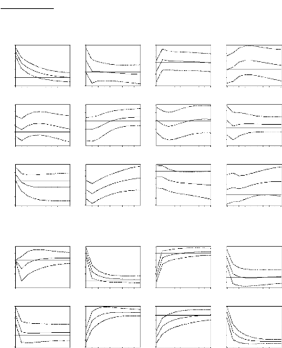
Response of FCT1 to FCT1

Response of FCT2 to FCT1

Response of FCT3 to FCT1

Response of FCT4 to FCT1

1 2 3 4 5 6 7 8 9 10

1 2 3 4 5 6 7 8 9 10

1 2 3 4 5 6 7 8 9 10

1 2 3 4 5 6 7 8 9 10

1 2 3 4 5 6 7 8 9 10

1 2 3 4 5 6 7 8 9 1

Response of FCT5 to FCT1

1 2 3 4 5 6 7 8 9 1

Response of FCT10 to FCT1

Response of FCT6 to FCT1

.8 .6 .4 .2

.0

-.2

-.4

0.8

0.4

0.0

-0.4

-0.8

-1.2

1 2 3 4 5 6 7 8 9 10

Response of FCT9 to FCT1

.4

.2

.0

-.2

-.4

-.6

2.0 1.5 1.0 0.5 0.0 -0.5 -1.0

-1.5

-2

-1

0

2

1

-3

0.5 0.0 -0.5 -1.0 -1.5 -2.0 -2.5

1 2 3 4 5 6 7 8 9 10

Response of FCT1 1 to FCT1

1 2 3 4 5 6 7 8 9 10

Response of FCT8 to FCT1

.8

.6

.4

.2

.0

-.2

-.4

-.6

Response of FCT12 to FCT1

1.2

0.8

0.4

0.0

-0.4

1 2 3 4 5 6 7 8 9 10

1 2 3 4 5 6 7 8 9 1

Response of FCT7 to FCT1

1.5 1.0 0.5 0.0 -0.5 -1.0

4

3

2

1

0

-1

2.0

1.2

0.8

0.4

0.0

-0.4

-0.8

.6

.4

.2

.0

-.2 -.4 -.6 -.8

ANNEXE 5 : Impulsions et réponses

Response to Cholesky One S.D. Innovations #177; 2 S. E.

Response of FCT5 to FCT2

Response of FCT6 to FCT2

Response of FCT7 to FCT2

Response of FCT8 to FCT2

Response of FCT1 to FCT2

Response of FCT2 to FCT2

Response of FCT3 to FCT2

Response of FCT4 to FCT2

Response to Cholesky One S.D. Innovations #177; 2 S. E.

0.4

0.0

-0.4

-0.8

-1.2

-1.6

-2.0

1 2 3 4 5 6 7 8 9 10

2.4

2.0 1.6 1.2 0.8 0.4 0.0 -0.4 -0.8

1 2 3 4 5 6 7 8 9 10

0.8 0.4 0.0 -0.4 -0.8 -1.2 -1.6

1 2 3 4 5 6 7 8 9 10

5

4

3

2

1

0

-1

1 2 3 4 5 6 7 8 9 10

1.0 0.8 0.6 0.4 0.2 0.0 -0.2 -0.4

2.4 2.0 1.6 1.2 0.8 0.4 0.0 -0.4

2

1

0

-1

-2

-3

-4

-5

-6

-7

0.5

0.0

-0.5

-1.0

-1.5

-2.0

-2.5

1 2 3 4 5 6 7 8 9 10 1 2 3 4 5 6 7 8 9 10 1 2 3 4 5 6 7 8 9 10 1 2 3 4 5 6 7 8 9 10

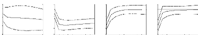
Response of FCT9 to FCT2

.4

.3 .2 .1 .0

-.1

-.2

-.3

Response of FCT10 to FCT2

3

2

1

0

-1

-2

Response of FCT1 1 to FCT2

1

0

-1

-2

-3

-4

Response of FCT12 to FCT2

0.5

0.0

-0.5

-1.0

-1.5

-2.0

-2.5

1 2 3 4 5 6 7 8 9 10

1 2 3 4 5 6 7 8 9 10 1 2 3 4 5 6 7 8 9 10 1 2 3 4 5 6 7 8 9 10 1 2 3 4 5 6 7 8 9 10

1 2 3 4 5 6 7 8 9 10

1 2 3 4 5 6 7 8 9 10

1 2 3 4 5 6 7 8 9 10

xxiv

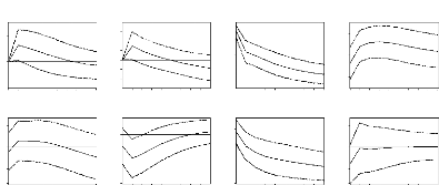
Response to Cholesky One S.D. Innovations #177; 2 S. E.

1 2 3 4 5 6 7 8 9 10

1 2 3 4 5 6 7 8 9 10

1 2 3 4 5 6 7 8 9 10

Response of FCT1 to FCT3

Response of FCT2 to FCT3

-0.4

-0.8

-1.2

0.8

0.4

0.0

1.2

1.6

Response of FCT5 to FCT3

Response of FCT6 to FCT3

-0.4

-0.8

-1.2

0.4

0.0

Response of FCT3 to FCT3

1.2

0.8

0.4

0.0

-0.4

Response of FCT7 to FCT3

4 3

2

1

0

-1

-2

1.2

0.8

0.4

0.0

-0.4

-0.8

.4 .3 .2 .1 .0

-.1

-.2

-.3

-.4 -.5

Response of FCT4 to FCT3

0.8 0.4 0.0 -0.4 -0.8 -1.2 -1.6

1 2 3 4 5 6 7 8 9 10

Response of FCT8 to FCT3

.4 .3 .2 .1 .0

-.1

-.2

-.3

-.4 -.5

1 2 3 4 5 6 7 8 9 10

1 2 3 4 5 6 7 8 9 10 1 2 3 4 5 6 7 8 9 10 1 2 3 4 5 6 7 8 9 10 1 2 3 4 5 6 7 8 9 10

1 2 3 4 5 6 7 8 9 10

1 2 3 4 5 6 7 8 9 10

1 2 3 4 5 6 7 8 9 10

Response of FCT9 to FCT3

Response of FCT10 to FCT3

Response of FCT1 1 to FCT3

Response of FCT12 to FCT3

Response of FCT9 to FCT3 Response of FCT10 to FCT3 Response of FCT1 1 to FCT3 Response of FCT12 to FCT3

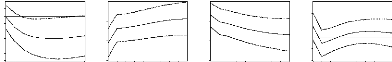
.2

.1 .0 -.1

-.2

-.3

-.4

-.5 -.6

1.2

0.8

0.4

0.0

-0.4

-0.8

1.5 1.0 0.5 0.0 -0.5 -1.0 -1.5

1.5 1.0 0.5 0.0 -0.5 -1.0 -1.5

1 2 3 4 5 6 7 8 9 10

1 2 3 4 5 6 7 8 9 10 1 2 3 4 5 6 7 8 9 10 1 2 3 4 5 6 7 8 9 10 1 2 3 4 5 6 7 8 9 10

1 2 3 4 5 6 7 8 9 10

1 2 3 4 5 6 7 8 9 10

1 2 3 4 5 6 7 8 9 10

Response of FCT7 to FCT4

Response of FCT5 to FCT4

Response of FCT8 to FCT4

Response of FCT10 to FCT4

Response to Cholesky One S.D. Innovations #177; 2 S. E.

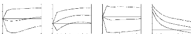
Response of FCT1 to FCT4

Response of FCT2 to FCT4

Response of FCT3 to FCT4

1.2

0.8

0.4

0.0

-0.4

-0.8

.3

.2

.1

.0

-.1

-.2

-.3

-.4

1.6

Response of FCT4 to FCT4

3.2 2.8 2.4 2.0 1.6 1.2 0.8 0.4 0.0 -0.4

.8

.4

.0

-.4

-.8

1 2 3 4 5 6 7 8 9 10 1 2 3 4 5 6 7 8 9 10 1 2 3 4 5 6 7 8 9 10 1 2 3 4 5 6 7 8 9 10

Response of FCT6 to FCT4

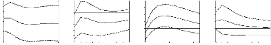
1 2 3 4 5 6 7 8 9 10

1 2 3 4 5 6 7 8 9 10

-0.2

-0.4

-0.6

-0.8

-1.0

0.4

0.2

0.0

1 2 3 4 5 6 7 8 9 10

1 2 3 4 5 6 7 8 9 10

.7

.6

.5

.4

.3

.2

.1 .0

-.1

4

3

2

1

0

-1

-2

.8 .6 .4 .2

.0

-.2

-.4

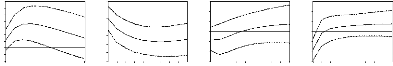
1 2 3 4 5 6 7 8 9 10

1 2 3 4 5 6 7 8 9 10

1 2 3 4 5 6 7 8 9 10

1 2 3 4 5 6 7 8 9 10

-0.5

-1.0

-1.5

-2.0

0.5

0.0

1.5

1.0

1.5 1.0 0.5 0.0 -0.5 -1.0 -1.5

.7 .6

.5

.4

.3

.2 .1 .0

-.1

-.2

1.2

0.8 0.4 0.0 -0.4 -0.8

-1.2

Response of FCT9 to FCT4

Response of FCT1 1 to FCT4

Response of FCT12 to FCT4

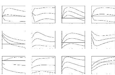
Response to Cholesky One S.D. Innovations #177; 2 S. E.

Response of FCT4 to FCT5

1 2 3 4 5 6 7 8 9 10

Response of FCT8 to FCT5

1 2 3 4 5 6 7 8 9 10

Response of FCT1 to FCT5

Response of FCT2 to FCT5

Response of FCT3 to FCT5

1 2 3 4 5 6 7 8 9 10

Response of FCT5 to FCT5

1 2 3 4 5 6 7 8 9 1

Response of FCT6 to FCT5

1 2 3 4 5 6 7 8 9 10

Response of FCT7 to FCT5

0.0

-0.4

-0.8

0.4

-1.2

1.2

0.8

0.4

0.0

-0.4

-0.8

0.8

1.0

0.8

0.6

0.4

0.2

0.0

-0.2

-0.4

1 2 3 4 5 6 7 8 9 10

1 2 3 4 5 6 7 8 9 10

1 2 3 4 5 6 7 8 9 10

4

3

2

1

0

-1

-2

Response of FCT1 1 to FCT5

1.2

0.8

0.4

0.0 -0.4 -0.8 -1.2 -1.6

1 2 3 4 5 6 7 8 9 10

1 2 3 4 5 6 7 8 9 10

1 2 3 4 5 6 7 8 9 10

Response of FCT9 to FCT5

.2

.1 .0

-.1

-.2

-.3

-.4

-.5 -.6

Response of FCT10 to FCT5

2.0

1.6

1.2

0.8

0.4

0.0

-0.4

-0.4

0.8

0.4

0.0

1.5

1.0

0.5

0.0

-0.5

1.2

0.8

0.4

0.0

-0.4

-0.8

.6 .4 .2

.0

-.2 -.4 -.6 -.8

Response of FCT12 to FCT5

1.0 0.5 0.0 -0.5 -1.0 -1.5 -2.0

1 2 3 4 5 6 7 8 9 10

Response of FCT12 to FCT6

1 2 3 4 5 6 7 8 9 10

Response of FCT1 1 to FCT6

1 2 3 4 5 6 7 8 9 10

3

2

1

0

-1

-2

1.6 1.2 0.8 0.4 0.0 -0.4 -0.8

Response of FCT7 to FCT6

Response to Cholesky One S.D. Innovations #177; 2 S. E.

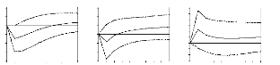
Response of FCT1 to FCT6

Response of FCT2 to FCT6

Response of FCT3 to FCT6

Response of FCT4 to FCT6

0.8 0.4 0.0 -0.4 -0.8

-1.2

.6 .5 .4 .3 .2 .1 .0

-.1

-.2 -.3

1.2

0.8 0.4 0.0 -0.4 -0.8 -1.2 -1.6

1 2 3 4 5 6 7 8 9 1

1 2 3 4 5 6 7 8 9 10

1 2 3 4 5 6 7 8 9 10

1.2

0.8 0.4 0.0 -0.4 -0.8 -1.2

1 2 3 4 5 6 7 8 9 10

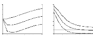
Response of FCT5 to FCT6

Response of FCT6 to FCT6

1 2 3 4 5 6 7 8 9 10

1 2 3 4 5 6 7 8 9 1

-0.4

2.4

2.0

0.8

0.4

0.0

1.6

1.2

.6

.4

.2

.0

-.2

-.4

-.6

1.5 1.0 0.5 0.0 -0.5 -1.0 -1.5

1 2 3 4 5 6 7 8 9 10

1 2 3 4 5 6 7 8 9 10

1 2 3 4 5 6 7 8 9 10

1 2 3 4 5 6 7 8 9 10

.6

.5 .4

.3 .2 .1 .0

-.1

-.2

0.4 0.2 0.0 -0.2 -0.4 -0.6 -0.8 -1.0

1.2

0.8

0.4

0.0

-0.4

-0.8

Response of FCT9 to FCT6

Response of FCT10 to FCT6

Response of FCT8 to FCT6

Response to Cholesky One S.D. Innovations #177; 2 S. E.

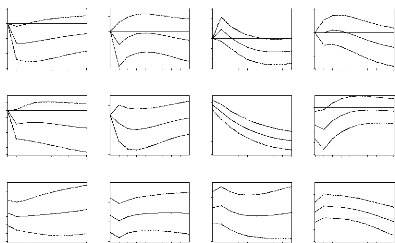
1 2 3 4 5 6 7 8 9 10

1 2 3 4 5 6 7 8 9 10

1 2 3 4 5 6 7 8 9 10

1 2 3 4 5 6 7 8 9 10

1 2 3 4 5 6 7 8 9 10

1 2 3 4 5 6 7 8 9 10

Response of FCT7 to FCT7

Response of FCT8 to FCT7

-2

-3

1.5

-0.5

0.0

1.0

0.5

-1

0

1

6 5 4 3

2

1 2 3 4 5 6 7 8 9 10

Response of FCT1 1 to FCT7

.2

.0

-.2

-.4

-.6

-.8

1 2 3 4 5 6 7 8 9 10

Response of FCT12 to FCT7

1.2

0.8

0.4

0.0

-0.4

-0.8

Response of FCT1 to FCT7

Response of FCT2 to FCT7

-.4

-.8

.4

.0

Response of FCT3 to FCT7

Response of FCT4 to FCT7

0.4

0.0

-0.4

-0.8

-1.2

0.8

.6 .4

.2

.0

-.2

-.4 -.6

0.4

0.0

-0.4

-0.8

-1.2

Response of FCT5 to FCT7

Response of FCT6 to FCT7

-.2

-.4

-.6

-.8

.2

.0

.4

Response of FCT9 to FCT7

Response of FCT10 to FCT7

-0.4

-0.8

-1.2

0.8

0.4

0.0

1.2

.2

.1

.0 -.1

-.2

-.3

-.4

-.5 -.6

.2

.1 .0

-.1

-.2

-.3

-.4

-.5

1 2 3 4 5 6 7 8 9 10

1 2 3 4 5 6 7 8 9 10 1 2 3 4 5 6 7 8 9 10 1 2 3 4 5 6 7 8 9 10 1 2 3 4 5 6 7 8 9 10

1 2 3 4 5 6 7 8 9 10

1 2 3 4 5 6 7 8 9 10

1 2 3 4 5 6 7 8 9 10

Response to Cholesky One S.D. Innovations #177; 2 S. E.

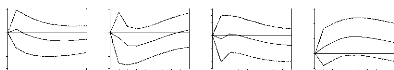
Response of FCT1 to FCT8

Response of FCT2 to FCT8

Response of FCT3 to FCT8

.4

.3 .2 .1 .0

-.1

-.2

-.3

-.4

-.5

-0.4

-0.8

-1.2

0.8

0.4

0.0

Response of FCT4 to FCT8

1.5

1.0

0.5

0.0

-0.5

0.8

0.4

0.0

-0.4

-0.8

-1.2

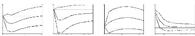
Response of FCT7 to FCT8

1 2 3 4 5 6 7 8 9 1

Response of FCT8 to FCT8

1 2 3 4 5 6 7 8 9 10

1.6

1.2

0.8

0.4

0.0

-0.4

1 2 3 4 5 6 7 8 9 10

1 2 3 4 5 6 7 8 9 10

Response of FCT5 to FCT8

Response of FCT6 to FCT8

0.2 0.0 -0.2

-0.4

-0.6

-0.8

-1.0

.4

.2

.0

-.2

-.4

-.6

3

2

1

0

-1

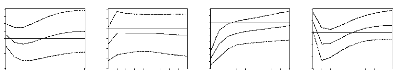
Response of FCT1 1 to FCT8

1 2 3 4 5 6 7 8 9 10

Response of FCT12 to FCT8

1 2 3 4 5 6 7 8 9 10

Response of FCT9 to FCT8

Response of FCT10 to FCT8

1 2 3 4 5 6 7 8 9 10

1 2 3 4 5 6 7 8 9 1

-0.4

-0.8

-1.2

-1.6

0.8

0.4

0.0

0.8 0.4 0.0 -0.4 -0.8 -1.2 -1.6 -2.0 -2.4 -2.8

.4

.3 .2

.1 .0 -.1

-.2

-.3

-.4

0.8

0.4

0.0

-0.4

-0.8

-1.2

1 2 3 4 5 6 7 8 9 10 1 2 3 4 5 6 7 8 9 10 1 2 3 4 5 6 7 8 9 10 1 2 3 4 5 6 7 8 9 10

Response to Cholesky One S.D. Innovations #177; 2 S. E.

Response of FCT1 to FCT9

Response of FCT1 to FCT9 Response of FCT2 to FCT9 Response of FCT3 to FCT9 Response of FCT4 to FCT9
Response of FCT2 to FCT9

Response of FCT3 to FCT9

Response of FCT4 to FCT9

1.2

.6

1.2

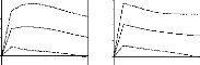
1.2

1.0

.4

0.8

0.8

.2

0.8

0.6

.0

0.4

0.4

0.4

-.2

0.2

0.0

-.4

0.0

0.0

-0.2

-.6

-0.4

1 2 3 4 5 6 7 8 9 10

1 2 3 4 5 6 7 8 9 10 1 2 3 4 5 6 7 8 9 10 1 2 3 4 5 6 7 8 9 10 1 2 3 4 5 6 7 8 9 10

1 2 3 4 5 6 7 8 9 10

1 2 3 4 5 6 7 8 9 10

1 2 3 4 5 6 7 8 9 10

Response of FCT5 to FCT9

Response of FCT6 to FCT9

Response of FCT7 to FCT9

Response of FCT8 to FCT9

Response of FCT5 to FCT9 Response of FCT6 to FCT9 Response of FCT7 to FCT9 Response of FCT8 to FCT9

.7

.4

2

.6 .5

.4

.3

.2

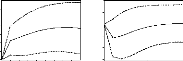
.6

.2

1

.5

.0

0

.4

.3

-.2

-.4

-.6

-1

.1 .0

-.1

.2

-2

-3

0.8

0.4

0.0

-0.4

-0.8

.1

.0

-.2

1 2 3 4 5 6 7 8 9 10

1 2 3 4 5 6 7 8 9 10

1 2 3 4 5 6 7 8 9 10

1 2 3 4 5 6 7 8 9 10

Response of FCT9 to FCT9

Response of FCT10 to FCT9

Response of FCT1 1 to FCT9

Response of FCT12 to FCT9

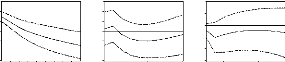
1.0

1.2 0.8 0.4 0.0 -0.4 -0.8

0.8

0.8

0.6

0.4

0.4

0.0

0.2

0.0

-0.4

-0.2

-1.2

-1.2

1 2 3 4 5 6 7 8 9 10

1 2 3 4 5 6 7 8 9 10 1 2 3 4 5 6 7 8 9 10 1 2 3 4 5 6 7 8 9 10 1 2 3 4 5 6 7 8 9 10

1 2 3 4 5 6 7 8 9 10

1 2 3 4 5 6 7 8 9 10

1 2 3 4 5 6 7 8 9 10

Response to Cholesky One S.D. Innovations #177; 2 S.E.

Response of FCT1 to FCT10 Response of FCT2 to FCT10 Response of FCT3 to FCT10 Response of FCT4 to FCT10

.8

0.8

.3

0.8

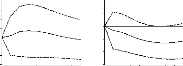
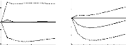
.6

.2

0.4

0.4

0.0

-0.4

-0.8

-1.2

.4

.1

0.0

.2

.0

.0

-0.4

-.1

-.2

-0.8

-.2

-.4

.6

-1.2

.3

1 2 3 4 5 6 7 8 9 10 1 2 3 4 5 6 7 8 9 10 1 2 3 4 5 6 7 8 9 10 1 2 3 4 5 6 7 8 9 10

Response of FCT5 to FCT10

Response of FCT6 to FCT10

Response of FCT7 to FCT10

Response of FCT8 to FCT10

.2

.6

1

.5

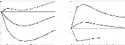
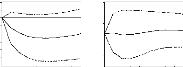
.1

.4

.3

.2

.4

.0

0

-1

-2

-3

1

0.8

0.4

0.0

-0.4

-0.8

1.2

.2

-.1

-.2

.0

.1

-.3

.0

-.2

-.4

-.1

-.4

-.5

-.2

-.6

-.6

-.3

1

2 3 4 5 6 7 8 9 10

1

2 3 4 5 6 7 8 9 10

2 3 4 5 6 7 8 9 10

1

2 3 4 5 6 7 8 9 10

Response of FCT9 to FCT10

Response of FCT10 to FCT10

Response of FCT1 1 to FCT10

Response of FCT12 to FCT10

.3

4

0.2

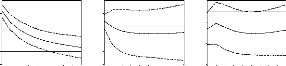
.2

0.0

3

.1

-0.2

.0

2

-.1

-0.4

1

-.2

-0.6

-.3

0

-0.8

-.4

-.5

1

-1.0

1

1 2 3 4 5 6 7 8 9 10 1 2 3 4 5 6 7 8 9 10 1 2 3 4 5 6 7 8 9 10 1 2 3 4 5 6 7 8 9 10
2 3 4 5 6 7 8 9 10

1

2 3 4 5 6 7 8 9 10

1

2 3 4 5 6 7 8 9 10

1

2 3 4 5 6 7 8 9 10

xxviii

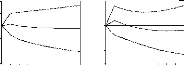
Response to Cholesky One S.D. Innovations #177; 2 S.E.

Response of FCT1 to FCT1 1 Response of FCT2 to FCT1 1 Response of FCT3 to FCT1 1 Response of FCT4 to FCT1 1
Response of FCT1 to FCT1 1

Response of FCT2 to FCT1 1

Response of FCT3 to FCT1 1

Response of FCT4 to FCT1 1

0.8

.4

0.5

0.8

0.4

0.0

-0.4

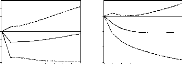
.3

0.4

.2

0.0

.1

0.0

.0

-0.5

-0.4

-.1

-.2

-1.0

-0.8

-0.8

-.3

-1.2

.4

1.5

-1.2

1 2 3 4 5 6 7 8 9 10 1 2 3 4 5 6 7 8 9 10 1 2 3 4 5 6 7 8 9 10 1 2 3 4 5 6 7 8 9 10
1

2 3 4 5 6 7 8 9 10

1

2 3 4 5 6 7 8 9 10

1

2 3 4 5 6 7 8 9 10

1

2 3 4 5 6 7 8 9 10

Response of FCT5 to FCT1 1

Response of FCT6 to FCT1 1

Response of FCT7 to FCT1 1

Response of FCT8 to FCT1 1

Response of FCT5 to FCT1 1 Response of FCT6 to FCT1 1 Response of FCT7 to FCT1 1 Response of FCT8 to FCT1 1

.4

.4

2

.3

.2

.1 .0 -.1

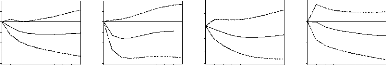
.2

.2

1

.0

.0

0

-.2

-.4

-.6

-.2

-.2

-.3

-.4

-.5

-1

-.4

-2

-.6

-.8

-.8

-3

.6

1 2 3 4 5 6 7 8 9 10 1 2 3 4 5 6 7 8 9 10 1 2 3 4 5 6 7 8 9 10 1 2 3 4 5 6 7 8 9 10

Response of FCT9 to FCT1 1

Response of FCT10 to FCT11

Response of FCT1 1 to FCT1 1

Response of FCT12 to FCT1 1

.5 .4

.3

.2

.1 .0

-.1

-.2

-.3

-.4

0.5

3.0

0.5

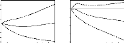
2.5

0.0

0.0

2.0

-0.5

1.5

-0.5

-1.0

1.0

-1.0

-1.5

0.5

-2.0

0.0

-1.5

1

1 2 3 4 5 6 7 8 9 10 1 2 3 4 5 6 7 8 9 10 1 2 3 4 5 6 7 8 9 10 1 2 3 4 5 6 7 8 9 10

2 3 4 5 6 7 8 9 10

1

2 3 4 5 6 7 8 9 10

1

2 3 4 5 6 7 8 9 10

1

2 3 4 5 6 7 8 9 10

Response to Cholesky One S.D. Innovations #177; 2 S.E.

Response of FCT1 to FCT12 Response of FCT2 to FCT12 Response of FCT3 to FCT12 Response of FCT4 to FCT12

.8 .6 .4

.2

1.0

.2

0.4

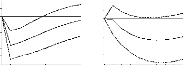
.1

0.2

0.5

.0

0.0

-.1

-0.2

0.0

-.2

.0

-0.4

-.3

-.2

-.4 -.6

-0.6

-0.5

-.4

-0.8

-.5

-1.0

.6

-1.0

1

1 2 3 4 5 6 7 8 9 10 1 2 3 4 5 6 7 8 9 10 1 2 3 4 5 6 7 8 9 10 1 2 3 4 5 6 7 8 9 10

2 3 4 5 6 7 8 9 10

1

2 3 4 5 6 7 8 9 10

1

2 3 4 5 6 7 8 9 10

1

2 3 4 5 6 7 8 9 10

Response of FCT5 to FCT12

Response of FCT6 to FCT12

Response of FCT7 to FCT12

Response of FCT8 to FCT12

Response of FCT5 to FCT12 Response of FCT6 to FCT12 Response of FCT7 to FCT12 Response of FCT8 to FCT12

.3 .2

.1 .0

-.1

-.2

-.3

-.4

-.5

.6

0.5

.5

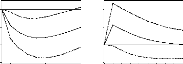
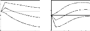
0.0

.4

.4

-0.5

.3

.2

-1.0

.2

.0

-1.5

.1

-.2

-2.0

.0

-.4

-2.5

-.1

-.6

-3.0

-.2

1

1 2 3 4 5 6 7 8 9 10 1 2 3 4 5 6 7 8 9 10 1 2 3 4 5 6 7 8 9 10 1 2 3 4 5 6 7 8 9 10

2 3 4 5 6 7 8 9 10

1

2 3 4 5 6 7 8 9 10

1

2 3 4 5 6 7 8 9 10

1

2 3 4 5 6 7 8 9 10

Response of FCT9 to FCT12

Response of FCT10 to FCT12

Response of FCT11 to FCT12

Response of FCT12 to FCT12

Response of FCT9 to FCT12 Response of FCT10 to FCT12 Response of FCT11 to FCT12 Response of FCT12 to FCT12

.2

2.0

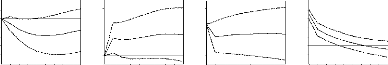
.4

1.2

.1 .0 -.1

1.6

1.2

.0

0.8

0.8

-.2

-.3

-.4

-.5

0.4

-.4

0.4

0.0

-0.4

0.0

-.8

-0.8

1

1 2 3 4 5 6 7 8 9 10 1 2 3 4 5 6 7 8 9 10 1 2 3 4 5 6 7 8 9 10 1 2 3 4 5 6 7 8 9 10

2 3 4 5 6 7 8 9 10

1

2 3 4 5 6 7 8 9 10

1

2 3 4 5 6 7 8 9 10

1

2 3 4 5 6 7 8 9 10

xxix

ANNEXE 5 bis :

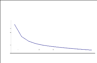
-0,2

1,4 1,2

1 0,8 0,6 0,4 0,2

0

1 2 3 4 5 6 7 8 9 10 11 12

Réponse de l'indice global suite à
l'impulsion de FCT1

xxx

des

~a61ematières

ii

iii

v

vi vii

1

3

4

4

5

7

7

8

8

9

10 11 13 13 13 13 13

13

14 16

16
17 22 22

22

22

23

23 24 24 24 24

Avant-propos

Dédicaces Remerciements Liste des abréviations et sigles Sommaire

Introduction ..

PARTIE I : CADRE THEORIQUE ET METHOD OLOGIE DE L 'ETUDE....... Chapitre 1 : Motivation et revue de littérature

Section 1 : Motivation

Section 2 : Revue de littérature .

Chapitre 2 : L'Indice Harmonisé des Prix à la Consommation

Section 1 : Définition de l'IHPC

Section 2 : Méthodologie d'élaboration des IHPC

A- Définition et description de l'univers .

B- Echantillonnage ..

C- Recueil et contrôle des données ..

D- Calcul de l'inflation

Chapitre 3 : Méthodologie de l'étude

Section 1: Saisonnalité et stationnarité ..

A- Saisonnalité

B- Stationnarité

1- Définition de la Stationnarité d'un processus

a- Stationnarité stricte

b- Stationnarité faible

2- Tests de stationnarité de Dickey-Fuller Augmentés .

a- Les processus TS

b- Les processus DS

Section 2 : Processus ARMA .

A- Identification ..

1- Identification à partir des corrélogrammes simple et partiel

a- Les processus AR(p)

b- Les processus MA(q)

c- Les processus ARMA(p,q)

2- Identification sur la base des critères de Akaïke et Schwarz

B- Validation ..

1- Tests sur les paramètres

2- Test de bruit blanc

PARTIE II : MODELISATION ET ANALYSE DES CHOCS

Chapitre 1 : Analyse descriptive des séries

1- Analyse de la fonction 1

2- Analyse de la fonction 2

3- Analyse de la fonction 3

4- Analyse de la fonction 4

5- Analyse de la fonction 5

6- Analyse de la fonction 6

7- Analyse de la fonction 7

8- Analyse de la fonction 8

9- Analyse de la fonction 9

10- Analyse de la fonction 10

11- Analyse de la fonction 11

12- Analyse de la fonction 12

Section 1 : Etude de la saisonnalité et de la stationnarité des séries

A- Analyse de la saisonnalité

B- Résultats de l'étude de la stationnarité

Section 2 : Identification, estimation et validation des modèles

A- Modèle de la fonction 1

1- Identification

2- Estimation et analyses

3- Interprétation de l'équation

B- Modèle de la fonction 2

1- Identification

2- Estimation et analyses

3- Interprétation de l'équation

C- Modèle de la fonction 3

1- Identification

2- Estimation et analyses

3- Interprétation de l'équation

D- Modèle de la fonction 4

1- Identification

2- Estimation et analyses

3- Interprétation de l'équation

E- Modèle de la fonction 5

1- Identification

2- Estimation et analyses

3- Interprétation de l'équation

F- Modèle de la fonction 6

1- Identification

2- Estimation et analyses

26

27

27

28

29

30

31

32

33

34

34

35

36

37

39

39

39

39

40

40

40

40

41

42

42

42

43

43

43

44 45 45 45

45

46

47

47

47

48

48

48 49

50

50

50

50

51

51

51

52

53

53

53

53

54

54

54

55
56 56 56

56

57 58 58

58

59 60

60

61

3- Interprétation de l'équation

G- Modèle de la fonction 7

1- Identification

2- Estimation et analyses

3- Interprétation de l'équation

H- Modèle de la fonction 8

1- Identification

2- Estimation et analyses

3- Interprétation de l'équation

I- Modèle de la fonction 9

1- Identification

2- Estimation et analyses

3- Interprétation de l'équation

J- Modèle de la fonction 10

1- Identification

2- Estimation et analyses

3- Interprétation de l'équation

K- Modèle de la fonction 11

1- Identification .

2- Estimation et analyses

3- Interprétation de l'équation

L- Modèle de la fonction 12

1- Identification .

2- Estimation et analyses

3- Interprétation de l'équation

Chapitre 3 : Analyse des chocs
Section 1 : Eléments théoriques sur l'analyse des chocs

Section 2 : Interprétation des réponses aux impulsions

. 62

Conclusion
Bibliographie

Annexes