Introduction
1 Negative density problem
The industry's standard SABR model (SABR stands for
Stochastic-Alpha-Beta-Rho) is a stochastic volatility model defined as
follows:
|
{ dFt =
ótFtâdWt1
dót =
áótdWt2
|
with d(W1, W2)t = ñdt
(1.1)
|
Where
· ñ E] - 1,1[ represents the link between the
forward and its volatility.
· â E [0, 1] is the elasticity of the forward's
backbone and is usually assumed constant, requiring then no calibration.
· á > 0 is the parameter that represents the
volatility of the volatility process.
Such a model presents a huge advantage because it takes into
account the randomness of the volatility parameter of a CEV process. It is then
crucial to be able to make a fair pricing under this model. A key is to rather
compute a lognormal implied volatility and then plug it into the Black-Scholes
formula in order to retrieve the price of the option.
In [26], Hagan et al. used singular perturbation
theory and found the following closed form formula for the implied volatility
in the SABR model
C z ~
óBS(K, F) = -

(FK)(1-â)/2 (1 +
(124)2 log2(F/K) +
(1-92ô4 log4(F/K) +
...) x(z)
ó0
- â)2á2
ñâíá2 - 3ñ2 2
C1 + [ (1
24(F/K)1-â +
4(FK)(1-â)/2 + 24 í ]
tex + ...
(1.2)
CHAPTER 1. PROBLEMS ENCOUNTERED WITH SABR
MODEL
v1-2ñz+z2+z-ñ
where x(z) = log(
1-ñ ) and z =
í á(F
K)(1-â)/2
log(F/K)
This formula has the advantage to be fast to compute and,
more, is a closed formula. Generally, closed formulas are preferred in the
financial industry because of their rapidness and few need of resources.
The same formula could also be obtained applying infinite
dimensional analysis and Malliavin calculus. In [34], the author considered a
slightly more general model which converges towards the original SABR model and
used a large deviation approach based on the non degeneracy of Malliavin
covariance. The Dynamic SABR model is rather used for FX Option markets.
Malliavin calculus can be used in a more general scope : the
decomposition of a process into consecutive Wiener chaos yields an exact
solution to all stochastic differential equations, provided they really have a
unique one [...].
However, even though this formula apparently suits to our
needs, it produces arbitrage for sufficiently low rates and long maturities.
That arbitrage is also observable when â is set to low values.
In order to highlight the arbitrage, let's compute the
probability density function of the underlying:
Let pF denote the underlying probability density function
(which is then supposed to exist) and PF the corresponding repartition
function.
If we compute the price of a call option under the suitable
forward probability QT, we'd have:
Ct = EQT
((FT - K)+
) t
|
?Ct
|
|
?
|
(FT1{FT
>K} - K1{FT >K})
|
|
?K =
|
?K
|
4
1. NEGATIVE DENSITY PROBLEM
|
?2Ct
?K2
|
= -EQT
(1{FT >K}) t
= -QT
(FT > K) Z +8
= - pF
(y)dy
K
[ ~
?
= PF
(K) -
lim
y?+8 PF
(y)
?K
|
=
pF(K)
Where Ct denotes the price of a European call option of strike
K, written on the underlying
(Ft)t.
Thus, for a set of strikes, we first compute implied
volatilities with Hagan formula, then price a set of calls for each strike, and
finally compute a numerical derivative of the call price twice according to the
strike.
The result is the so-called probability density that we have
plotted in the following picture for several maturities.
1. NEGATIVE DENSITY PROBLEM
5
CHAPTER 1. PROBLEMS ENCOUNTERED WITH SABR MODEL
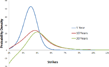
Figure 1.1: F0 = 0.0325, ó0 = 0.087,
á = 0.47, â = 0.7, ñ = -0.48
Indeed, as we can see it on the above picture, we may have
some negative densities while increasing the option's maturity.
In order to improve the accuracy of the implied volatility
approximation, Henry Labordere used a heat kernel expansion on a Riemann
manifold endowed with an Abelian connection in [27] and found an approximation
for a more general scope of stochastic volatility models. Applying this
asymptotic development to SABR model yields:
óN(K,T) = S0(K)(1 + TS1(K)) (1.3)
where
1 (x l aauñsinh(d(x))
- 1 S0(x)2xF
S0(x) = S(x) log \Fl , 8 (x) _ 4
(/Eâ-1) d(x) 28(x)2 log
a(x)a(F)xâFâ
q
á(x1-â - F
1-â)
q(x) = 1 - â , a(x) = óô +
q(x)2 + 2ó0ñq(x)
S(x) = 1 log q(x)
u+ o(1 o-0+p +pp) a(x)
d(x) = argch -q(x)ñ -
ó0ñ2 + a(x)
á ó0(1 -
ñ2)
N/
~ = KF
The above implied volatility is a normal one, i.e. retrieved
from an inversion of the pricing formula in the Bachelier Model. For
comparison, we can approximately find back a Black-Scholes implied volatility
through the following equivalence:
|
óN =
|
2 ~S-K ~
3
V'
S - K log KS(log S-log K)
2 2
log S - log K óLN 1 -(log S
- log K)2 óLNT + O (T log(T)
(1.4)
|
CHAPTER 1. PROBLEMS ENCOUNTERED WITH SABR
MODEL
In particular, uN ~ S-K
log S-log K óLN when T
? 0. We gave a detailed proof of this
equivalence in Appendix B.
The following picture shows how Labordere's approximation
improves the accuracy of implied volatility asymptotics.
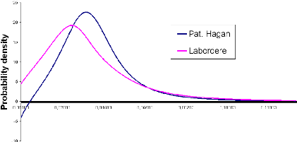
Figure 1.2: F0 = 0.0325, u0 =
0.087, á = 0.47, 9 = 0.7, p = -0.48, T = 15Y
For a 15 years expiry, the negative densities observed with
the Hagan expansion simply vanish. Despite that accuracy, for a sake of rigor,
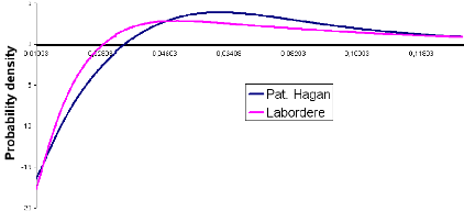
we make some model parameters "worse" and track the behaviour of the
probability density. We know that a SABR model with parameter 9 = 1 and
constant volatility is identically a Black-Scholes model. We can therefore
reasonably expect the model to spread from the basic Black-Scholes when 9 ? 0.
In the following picture, we choosed 9 = 0.4: let's see what happens.
6 1. NEGATIVE DENSITY PROBLEM
Figure 1.3: F0 = 0.0325, u0 =
0.087, á = 0.47, 9 = 0.4, p = -0.48, T = 15Y
CHAPTER 1. PROBLEMS ENCOUNTERED WITH SABR
MODEL
As we can remark it, both Hagan and Labordere approximations
fail under extreme conditions. This is not really surprising since those
formulas are simply short-maturity expansion results. Hence, we address a more
qualitative question: which one practitioners prefer between fast to compute
approximations and heavy accurate calculus ?
The SABR model can be used to accurately fit the implied
volatility curves observed in the marketplace for any single exercise date.
More importantly, it predicts the correct dynamics of the implied volatility
curves. This makes the SABR model an effective means to manage smile risk in
markets where assets only have a single exercise date; these markets include
swaption ans caplet/floorlet markets.
2 Wings Control
We now address the issue of wings control. The price of
illiquid assets extremely depends on the shape of the implied volatility wings.
This is for example the case of the price of a CMS, specially due to the
computation of convexity adjustments. A high out-of-money implied volatility
yields high prices.
Here is for example how SABR parameters control the smile: The
lower we set á, the more we spread the smile...
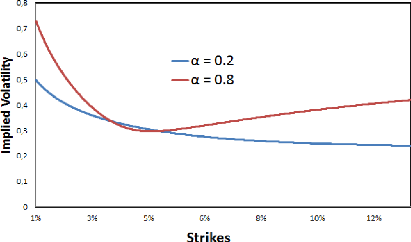
Figure 1.4: F0 = 0.0325, u0 = 0.087, â = 0.7, p = -0.48,
T = 15Y
2. WINGS CONTROL 7
The higher we set â, the flatter the smile gets...
8 2. WINGS CONTROL
CHAPTER 1. PROBLEMS ENCOUNTERED WITH SABR
MODEL
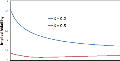

Figure 1.5: F0 = 0.0325, ó0 = 0.087,
á = 0.47, p = -0.48, T = 15Y
This is not surprising since for 9 = 1 and a constant volatility,
we face a Black-Scholes model and the latter produces nothing but a flat smile
!
Increasing p rotates the smile in a counter-clockwise
direction.
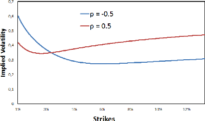
Figure 1.6: F0 = 0.0325, ó0 = 0.087,
á = 0.47, 9 = 0.7, T = 15Y
We therefore focus on finding other model parameters, or at
least, adapted transformations of SABR model that may provide additional
control features.
2. WINGS CONTROL 9
CHAPTER 1. PROBLEMS ENCOUNTERED WITH SABR
MODEL
Practitioners usually focus on changing the backbone shape of
SABR model, that is, the curve of ATM implied volatilities for different
strikes. In order to add more control parameters to the model, we can replace
the ?(F) = F'3 in the underlying SDE
by:
· ?(F) = F'3(F) with
â(F) = â0 + (â8 -
â0) (1 - e-F/Fmax)
where Fmax is typically much larger than the forward
rate F0. This gives a control on the upper-wing of
the smile.
· ?(F) = F'3 x
(F/F1)$1+1
(F/F2)$2+1. This
parametrisation allows us to control both lower
and upper wings.
· ?(F ) = F $1
1+F$1-$2 .
The later was suggested to me by the Fixed Income Derivatives
Quants of Crédit Agricole, and has the particularity to converge to
different SABR models. Indeed,
(1.5)
F '31
lim ?(F) = lim = F'32
F?+8
F?+8 1 +
F'31-'32
F '31
lim ?(F ) = lim = F '31
F ?0
?0
F 1 +
F'31-'32
This model tends then to a
SABR(â1) for low values of the forward and a
SABR(â2) for high forwards.
Despite those improving attempts, practitioners still face a
major problem: the above listed backbone transformations lead to a full control
of the smile, both liquid and illiquid regions. As highlighted in the
introduction, models are needed for illiquid assets; however, models should
first behave well for liquid assets for a sake of calibration. If one modifies
SABR's behaviour for the whole smile, one although fits illiquid region's
behaviour but also loses the liquid region's behaviour. This is therefore a
destruction of the cornerstone of our model.
What we need is another model that provides a real parameter
for wings control without changing the model's behaviour for liquid assets. We
will therefore propose a new model which is able to change wings without
(sensibly) touching the liquidity region.
| 

