Zabr modelling

Conclusion

In addition to the negative density problem for very in-the-money vanilla options, the SABR model lacks an additional control parameter for very out-of-money options.

In the next chapter we will expose solutions for both of these problems. We shall develop a Normal SABR model which solves the negative density problem, and then study the ZABR model that controls the wings.

CHAPTER 1. PROBLEMS ENCOUNTERED WITH SABR MODEL

10 2. WINGS CONTROL

11

Chapter 2

Normal SABR

Introduction

As mentioned in the previous chapter, problems with the SABR implementation through the Hagan expansion, such as the breakdown of the expansion for high volatility and the possibility of negative probabilities for very low strikes, did not matter at the time but now constitute a pressing problem for the swap and rates options markets. In this chapter, we present a solution to these problems based on Philippe Balland and Quan Tran expansion (see [7])

The SABR backbone function ?(.) satisfies the usual linear growth and Hölder continuity conditions to ensure that the SABR stochastic differential equation admits a unique solution when appropriate boundary conditions are specified.

In the original dynamics, ?(F) = Fâ and the forward rate is assumed to be absorbed at zero. The constant elasticity of variance (CEV) â is typically greater than zero and smaller than one in interest rate applications. Negative rates can be accommodated by assuming that (Ft + Ä)t follows SABR dynamics. The model is very popular among practitioners because it provides an intuitive parametrisation of volatility smiles.

Unfortunately, the asymptotic formula derived by Hagan et al. (2002) loses accuracy for long-dated expiries, especially when the CEV exponent is close to zero or when the volatility-of-volatility is large. This loss of accuracy is problematic from a practical point of view because the density can become negative near the forward. New techniques have recently been proposed to improve the accuracy in the original expansion of the implied volatility. When the correlation is zero, Antonov & Spector [35] derived an exact expression for the price of a vanilla option based on a double integral. When the correlation is non-zero, the authors proposed using an approximately equivalent SABR model with zero correlation.

Small CEV exponents are typically used to represent swaption and caplet smiles at the long end of the curve, where the asymptotic formula also breaks down. Based on this observation, we perform an asymptotic expansion of the implied volatility corresponding to Normal SABR with absorption at zero, instead of Black-Scholes. We find that the resulting approximation is more accurate than the original SABR

and the measure d Q

dQ

Q except for the drift of ót:

ñt. We note that Jt has the same dynamics under Q and

12 1. EQUIVALENT SABR. LOCAL VOLATILITY

CHAPTER. 2. NOR.MAL SABR.

expansion and results in significant calculation time saving when compared with solving the one-factor equivalent local volatility PDE.

1 Equivalent SABR local volatility

As explained in [15] and [25], we can obtain an accurate approximation of the local volatility equivalent to SABR. The local volatility g(t, K) for SABR is given by the following expression:

g(t, K)² = ?(K)²E [ó2 _t ä (Ft - K)] (2.1)
E [ä (Ft - K)]

We denote the numerator of this expression (the so-called local time) by Lt, and the denominator (the process's probability density) by Dt. In this section, we derive an approximation for g(t, K) by simple applications of Itô's lemma and Girsanov's theorem. We have included this derivation as it will serve as the basis for our normal SABR expansion.

The SABR local time Lt is approximated by introducing the process:

1 du

J(Ft,ót) =ót jFt

(u) (2.2)

and observing that:

Lt = ó0?(K)E [e^áWt2-2tä(Jt)] (2.3)
By applying Itô's lemma and performing the change of measure dbQ

dQ = _eáWt²-2¹á²t,

we derive:

Lt = ó0?(K)

bE [ä(Jt)]

1 (2.4)

dJt = \/q(Jt)d^cWt - 2 ÿ?(Ft)ótdt

where q(J) = 1 - 2ñáJ + á²J² and _(Wt)t is a brownian motion under ^bQ.

The SABR density Dt is similarly approximated by performing the change of

-áWt2-21á2t :

E [ä(Jt)/ót]

D=

?(K)

=

measure dQ

dQ = e

E [ä(Jt)]eá2t

ó0?(K) (2.5)

_p

dJt = q(Jt)d Wt + ÿq(Jt)dt - 21 ÿ?(Ft)ótdt We define the martingale:

dñt ÿq(Jt)

= d W (2.6)
ñt Nq(Jt)

CHAPTER 2. NORMAL SABR

1 !

Z t ÿd(Ju)

Xt = ñt exp ÿ?(Fu)óuq(Ju)du (2.7)

2 0

It follows that the SABR density satisfies:

_i

E hq(J0) _eá²t
q(Jt)ä(Jt)

q(J0)ó0?(K)

Dt =

=

E hexp C2 R0 ^ÿ?(Fu)óu^ÿq_qt du) /Jt = 0i

×

q(J0)ó0?(K)

(2.8)

E [ä(Jt)]

Since the volatility ót only appears in the drift expression of Jt, we conclude that

^bE[ä(Jt)] E[ä(Jt)]

= 1 + O(t²). We consequently have:

g(t, K)² = q(J0)ó20?(K)2e 2 ⁽ñáÿ?(K)-21ÿ?(F0)Z0)⁾t + O(t²) (2.9)

We finally derive the following first-order approximation in time of the SABR local volatility:

_p

g(K) = ó0?(K) 1 + 2ñáf(K) + á²f(K)²,

Z K

1 du (2.10)

f(K) = ó0 ?(u)

F0

Using this equivalent local volatility, we obtain Hagan's first order approximation for the implied volatility under SABR using standard results for local volatility:

ln (K/F0) =(2.11)

R f(K;?) dí

0 v1+2ñáí+á2í2

ln (K/F0)

IV (K; ?, á, ñ) =

RK du
0 g(u)

The SABR local volatility behaves like a CEV dynamic near zero. The absorption at zero is ignored in the above approximation because we are using Black-Scholes as the base model for our implied volatility calculation. Hence, we can expect to improve accuracy by choosing a base model with a dynamic absorbed at zero.

2 Asymptotic expansion with different base models

Suppose that we can accurately integrate the following instance of the SABR dynamics:

? ???? ????

dFt = ót?^base(Ft)dWt^1dót = áótdWt^2 ót=0 = b0

(2.12)

where á and ñ are as in SABR. By matching the first-order implied volatility approximations, that is, IV (K; ?base, á, ñ) = IV (K; ?, á, ñ), we derive the base

2. ASYMPTOTIC EXPANSION WITH DIFFERENT BASE MODELS 13

CHAPTER 2. NORMAL SABR

implied volatility b0 so that the base model and SABR share the same implied volatility to first order in time:

u

ó0(1 - r

JF^K0 (Pbas^de(u)

b0 = (2.13)

K1-â - F1-â

0

We consider two base candidates. Our first one is SABR with shifted lognormal backbone:

?

base 1 (F) = pF + (1 - p)F0 (2.14)
This base dynamics can be integrated by inverting a Laplace transform. Al-

though tractable, this requires a double integration.

Our second candidate is normal SABR with absorption at zero:

?base 2 (F) = lim â?0

Fâ = 1{F>0} (2.15)

We will see in the next section that SABR with a normal backbone can be accurately approximated with limited calculation cost. We observe that the initial normal volatility to use when approximating SABR with this base model is as follows:

ó0(1 - â)(K - F0)

b0 = (2.16)
K1-â - F 1-â

0

In the case where we attempt to approximate SABR with an extended backbone ?(.) instead of a CEV backbone, then our formula for b0 is generalised as follows:

ó0(K - F0)

(2.17)

b0 = _rK du

JF0 ?(u)

As observed in [4], the SABR dynamics calibrated to swaption smiles do not imply Constant Maturity Swap (CMS) levels consistent with the market. Various methods have been proposed to address this issue. These attempts to steepen the upper-strike wing while not affecting the liquid region and the lower wing too much. They are based on modifying either the density, conditionally to being in the upper-wing or directly the SABR dynamics.

We can gain control on the upper-wing steepness by assuming the following backbone:

?(F) = Fâ(F)

F~F~, a~ (2.18)

â(F) = â0 + (â₈- â0)(1 - e- )

where Fmax is typically much larger than the forward rate F0 in order to localise the effect of double beta to the high-strike wing.

An alternative is to use the following double-beta backbone to control both lower and upper wings:

?(F) = F^â x (F/F1)â¹ + 1 (2.19)

(F/F2)â² + 1

14 2. ASYMPTOTIC EXPANSION WITH DIFFERENT BASE MODELS

CHAPTER 2. NORMAL SABR

This parametrisation allows us to account for the extra risk premium for high-strike volatilities and for the fact that traders typically increase â when interest rates become very low.

3 Approximation for normal SABR

We obtain the following formula for a call option under the normal SABR model by applying the Tanaka-Meyer formula to a call payout (see [8]):

T

E[(FT - K)⁺] = (F0 - K)⁺ + 2 J b²₀E [u²_tä(Ft - K)] dt (2.20)

0

where ut = ót/b0 with ó0 = b0. We observe that:

E [u²_t ä(Ft - K) = E [utä(Xt)]

Xt = Ft - K (2.21)

ut

Finally, we denote by Pu the probability measure associated with the Radon derivative ut = ót/b0 and obtain the following formula for a call option under normal SABR:

T

E[(FT - K)⁺] = (F0 - K)⁺ + 2 Z bE^u [ä(Xt)] dt (2.22)

The process _(Xt)t satisfies:

_p

dXt = b0 q(Xt)dW u (2.23)

t?ô

where q(X) = 1 - 2ñáX + á²X², á = á/b0 and r is the first time F hits zero.

The stopping of the diffusion is a consequence of using SABR with vanishing CEV coefficient. As explained in [25], accounting for this stopping is important because the support of SABR is the positive half line and our base model must share with SABR the same behaviour at zero otherwise our lower-strike wing will be too steep. The importance of using interest rate models with absorbing and reflecting boundaries is discussed in [12].

Ignoring the volatility-of-volatility, we approximate r as the first time X hits its expected barrier level under Pu, at which point X_ô = Eu [-K/ut] = -K. This approximation does not compromise the accuracy of our call price because it only affects option prices with very low strikes. We can gain additional control on the lower-wing steepness by assuming that X is absorbed at the level Fmin - K where Fmin = (p - 1)/pF0 is negative, that is, 0 < p < 1.

We define the following process:

!

xt

It = I(Xt) = / du = 1 ln q(Xt) - ñ + áXt (2.24)

o q(u) á 1 - ñ

We can derive an approximation for the density of _(Xt)t at zero using the reflection principle for Brownian motion (see Appendix A):

3. APPROXIMATION FOR NORMAL SABR 15

CHAPTER 2. NORMAL SABR

Eu [ä(Xt)] = q(X0)14

b0 v2ðt

~ ~

e- ^B2

b2 0t - e-

b2

× Ë(t) × 0t

16 4. PRICING FORMULA WITH NORMAL SABR AS BASE

I(F0 - K) 2I(Fmin - K) - I(F0 - K)

B = v2 , C = v2 ~ ~ Ë(t) e- 8 á2t × Ö ^1t, I0 b0 ~ 3 Z t ~ ~ du Ö(t, z) = E exp 8á^2(1 - ñ^2) /Wt = z f(Wu) 0 1 ~(1 + ñ)^2e^-2áW+ (1 - ñ)^2e^2áW+ 2(1 - ñ^2)~ f(W) = 4

(2.25)

Hence, we obtain the following approximation for call prices under SABR:

2 _C2

E[(FT - K)⁺] = (F0 - K)⁺ + q(F0 - K)1/4b0 T1ef0 _,L e° (e b20t - e ^b20t) dt

2v2ð o t

ó0(K - F0) b0 = R K du

F0 ?(u)

ê(t, z) = -₈á² + ?tlnÖ(t, z) 1

(2.26)

The function ê(t, z) is independent of K and only depends on the SABR parameters á and ñ.

~ 1 ~

1 3 1

^{2 2 2}

(2.27)

We have the following first-order approximation:

Ö(t, z) = exp [-¹₈á²t

+ ₁₆á²(1 - ñ2) C f(0) + f(z)/

_t]

+ O(t²)

We can estimate ê(t, z), Ö(t, z) more accurately without any major increase in calculation time. First, we pre-compute by forward induction Ö (Ti,îjvTi) on a fixed-time grid {Ti}i<N and an N(0, 1)-mesh {îj}j<M as explained in Appendix A.

~ ~

Finally, we approximate ê s, ^I0 by a constant êi over each interval _(Ti-1, Ti): b0

êi 1 2 = -8á +	h ~ i h ~ i ln Ö Ti, ^I0- ln Ö Ti-1, ^I0 b0 b0		(2.28)

where Ö(Tk, z) is obtained by cubic spline interpolation of {Ö (Tk, îjvTk) : j = 0,..., M - 1}.

4 Pricing formula with normal SABR as base

From our previous calculations, we derive the following approximation for the price of an option on a SABR underlying _(Ft)t using normal SABR as a base for our asymptotic expansion:

CHAPTER 2. NORMAL SABR

N

E[(FT-K + = (F0 - K)^#177; + q(F0 - K)1/4b é (âa²+~z)Ti 1~ (T Io × J

) ) 2v2ð _o ( Z-1 bo / i

i=1 \

Ji =

1 Z Ti 1 vt 2 Ti-1

~ ~ e- ^B2 eêit b2 0t - e- ^C2 b2 0t dt

(2.29)

The above integrals Ji are calculated using formula (7.4.33) in [20]:

_I

~ ~v ~ ~~

+ e-2|ë|v-ê -êT - |ë|

erf v + 1

T

_T r2 ~_te^êu-û² du ^=Le2|ë|v-ê (erf (-êT + - T(2.30)

where

Z x ~ v ~

2

erf(x) = _?ð e^-t2dt = 2N x 2 - 1 (2.31)

0

and v-ê is either imaginary or real. The error function with complex argument can be estimated using the infinite series approximation of Abramowitz & Stegun (see formula 7.1.29 in [20]) as suggested in [8]:

+8

e

x2 2

-

_n2

-

n2 + 4x2 (f_n(x, y) + ig_n(x, y))

e

4

X

_e-x²

erf(x + iy) = erf(x) + _2ðx (1 - cos 2xy + isin2xy) + ð

n=1

f_n(x, y) = 2x - 2x cosh(ny) cos(2xy) + n sinh(ny) sin(2xy) g_n(x, y) = 2x cosh(ny) sin(2xy) + n sinh(ny) cos(2xy)

(2.32)

In practical application, it is sufficient to include the first 10 terms to ensure a very good accuracy. From the above expression, we can calculate analytical expressions for the cumulative and density functions.

In the following picture, we have plotted the implied density obtained when pricing under Normal SABR. For a sake of comparison, we have also plotted densities obtained from Hagan and Labordere approximations.

4. PRICING FORMULA WITH NORMAL SABR AS BASE 17

18 4. PRICING FORMULA WITH NORMAL SABR AS BASE

CHAPTER 2. NORMAL SABR

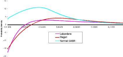
Figure 2.1: F0 = 0.0325, u0 = 0.087, á = 0.47, 9 = 0.4, p = -0.48, 'y = 1, T = 15Y

Indeed, the negative density problem is solved, even for extreme model parameters.

The main drawback is a high computation time, mainly due to the computation of transition probabilities. The latter is however performed once for all strikes.

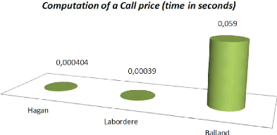
Figure 2.2: F0 = 0.0325, u0 = 0.087, á = 0.47, 9 = 0.4, p = -0.48, 'y = 1, T = 15Y

The above picture shows how much time it actually takes to price under Normal SABR. This pricing takes 200 times more time than the Hagan and Labordere approximations but that is the price we pay in order to eliminate arbitrage.

4. PRICING FORMULA WITH NORMAL SABR AS BASE 19

CHAPTER 2. NORMAL SABR