Zabr modelling

Conclusion

The Normal SABR model solves the negative density problem observed with the Hagan approximation. However, it introduces another issue, the excessive computation time for pricing. Indeed, practitioners prefer closed form formulas for pricing (such as Black-Scholes) and changing the whole pricing kernel can quickly become a trip to Pandemonium. Moreover, solving only the negative density problem leaves untouched the wings control one. In the next chapter, we will introduce a wings controlling model and show how to compute arbitrage-free prices.

CHAPTER 2. NORMAL SABR

20 4. PRICING FORMULA WITH NORMAL SABR AS BASE

Chapter 3

The ZABR model

Introduction

Interest rate option desks typically need to maintain very large amounts of inter-linked volatility data. For each currency, there might be 20 expiries and 20 tenors, that is, 400 volatility smiles. Furthermore, the smiles might be linked across different currencies. Interpolation of observed discrete quotes to a continuous curve is needed for the pricing of general caps and swaptions. At the same time, extrapolation of options quotes is needed for constant maturity swap (CMS) pricing. For these purposes, the industry uses to approximate SABR model using expansions as in [26]. The implied volatility expansions have the advantages that they are fast and simple to code but as mentioned in the previous chapter, these expansions are not very accurate, particularly not for long maturities nor low strikes.

With the low rates we have today, this problem is more acute than ever. Furthermore, the SABR model only has four parameters to handle the above-mentioned tasks, which is not enough flexibility to exactly fit all option quotes. In this chapter, we extend the stochastic volatility process to include a constant elasticity of variance (CEV) skew on the volatility of volatility. The CEV volatility process allows us to have more explicit control of the extrapolated high-strike volatilities, which in turn allows better control of CMS prices. Further, we will use a non-parametric volatility function for the spot process, which enables us to have an exact fit to all the observed quotes and gives us the ability to model negative option strikes.

In this chapter, instead of buying into heat kernel expansions, we use a short-maturity expansion for the implied volatility of the option. The short maturity expansion also yields results for the short-maturity limit of the Dupire forward volatility ( [11]), that is, the short-maturity limit of the conditional expected local variance

V(F)^2= uim t?0

] dhF it dt /Ft = F (3.1)

21

We provide two procedures to directly calibrate the model to observed CMS prices: an implicit method that works by iteration of the connection from parameters to price in a non-linear solver (see Section 3.3), and a direct method that infers the

22 1. SHORT MATURITY EXPANSION

CHAPTER 3. THE ZABR MODEL

parameters of the model from an arbitrage-free continuous curve of option prices (see Section 5).

1 Short maturity expansion

We consider the slightly more general model:

( dFt = ót?(Ft)dW_t¹

with d(W¹, W²)t = ñdt (3.2)

dót = c(ót)dW_t²

The non-parametric form of the volatility function ?(.) allows us to have a perfect fit to any discrete or continuous set of observed arbitrage-free options quotes. We can write the price of an European call option on a fixing FT as:

Ct = E [(FT - K)⁺ /Ft] = g (t, Ft, v(t))

where v(t) is the implied normal volatility and g is the normal (Bachelier) option pricing formula:

g(ô, x, v) = (x - K)JV x - K + vôfv.Vô)z ^Cv~K) , ô = T - t (3.3)
Applying Itô's lemma to 3.3 yields:

dCt = -g_ôdt + gxdFt +1

gxxd(F)t + gvdvt + _2gvvd(v)t + g_xvd(F, v)t (3.4)
where subscripts denote partial derivatives. In the following, we assume vt > 0 Define Xt = Ft-K. Using Itô's lemma yields:

vt

1 dXt = vt

dFt -Ft 2^Kdvt - 2d(F,v)t + Ft -3Kd(v)t vt vt vt

(3.5)

(3.6)

1

= (dFt - Xtdvt) + O(dt)
vt

d(X)t = v2 (d(F)t + Xt d(v)t - 2Xtd(F, v)t)

t

2

gxx

gxx

The normal option pricing function, g, has the following properties:

g_v = vôgxx

Cx - K

gvv = v

x - K

v

gxv =

1

0 = -g_ô + ₂v²gxx

Using the above properties, we can transform equation 3.4 into:

1. SHORT MATURITY EXPANSION

23

CHAPTER 3. THE ZABR MODEL

1 ]

dCt - gxdFt = 2gxx [v2 t (d(X)t - dt) + 2ôvdvt (3.7)
The left hand side of 3.7 is the change in value of a hedged portfolio. Taking conditional expectations yields:

1

0 = ₂gxxv²

1 t E (d(X)t - dt/Ft) + gxxôvtE (dvt/Ft) (3.8)
For small maturities, ô -+ 0, and we have

₂gxxv²t E (d(X)t - dt/Ft) 0 (3.9)

As gxx > 0 for v > 0, and for any diffusion, E (d(X)t - dt/Ft) = 0 is equivalent to d(X)t = dt, we obtain the arbitrage condition:

d(X)t		= 1 (3.10)	dt

Note that this is a diffusion condition rather than the drift condition that we normally see in financial mathematics. As the function X H X(f, ó) must be a function of the state variables (Ft, ót), the diffusion condition 3.10 leads to the differential equation:

1 = (XfdFt + X_ódót)²

dt (3.11)
= ó²_t ?(Ft)²X²_f + E(ót)²X²_ó + 2ñót?(Ft)c(ót)XfX_ó

Given the function ?(.), we need to solve this non-linear first order differential equation subject to the boundary condition X(f = K, ó) = 0. Once we have the solution X(f, ó), we can find the implied volatility as:

F - K

=

v(3.12) X(F,ó0)

We note that the error of the implied volatility is O(ô). The result implies that for any choice of ?(F), any function X = X(f, ó) that satisfies d(X)t = dt leads to an implied volatility given by v = (F - K)/X.

We could have chosen to derive the short-maturity expansion in implied Black-Scholes (lognormal) volatility v instead of implied normal volatility. Instead of X,

we should then have chosen the transformation

. The diffusion condi-

X = ln(F/K)

v

tion would be the same so X = X. This relates short-maturity implied lognormal and normal volatilities, as in Appendix B (first order equivalence), by the simple relationship:

v ln(F/K)

= (3.13)

v F - K

The expansion results that we present in the following can easily be switched between use in implied normal and implied lognormal volatility form by use of equivalence formulae.

CHAPTER 3. THE ZABR MODEL

2 Application to benchmark models

Before we address the very ZABR model results, we first of all apply the short-maturity expansions from the previous section to well known models. Those models can be retrieved while varying the function c(.).

2.1 Local Volatility model : case ~(ót) = 0

In this case, ót = 1, and the differential equation 3.11 reduces to ordinary differential equation (ODE):

X²_f?(F)² = 1 (3.14)

Using the boundary condition X(F = K) = 0, we find the solution:

Z F 1 X = ?(u) K

du (3.15)

v = v =

with corresponding implied normal and Black volatilities given by:

F - K

f F K ?(u)du

1

(3.16)

ln(F/K)

f F K ?(u)du

1

These results appear in many places, for example in [19]. We note that 3.15 implies the following relationship between X and the forward volatility:

?X ?K =

1 (3.17) ?(K)

Suppose we have X from a stochastic volatility model like 3.2, that is, given as the solution to 3.11 for some volatility functions ?(F), c(ó) and correlation ñ. Let's define the function V by:

~?X ~-1

V(K) = - (3.18)

?K

and consider the deterministic local volatility model:

dFt = V(Ft)dWt (3.19)

It now follows that:

XLV =

Z S K

V(u)^-1du = X (3.20)

24 2. APPLICATION TO BENCHMARK MODELS

So the stochastic volatility model 3.2 and the local volatility model 3.19 will produce the same short-maturity expansion option prices.

The above is a short-maturity limit version of the general result by Gyongy and Dupire (see [13] and [6]), that the model:

CHAPTER 3. THE ZABR MODEL

dFt = a(t, Ft)dWt , F0 = F0 (3.21)

produces the same option prices as the model 3.2 if a(., .) is chosen to be:

~dhF it ~

a(t, k)² = E dt /Ft = k (3.22)

We conclude that in the short-maturity limit, the conditional expected variance of the underlying is related to the transformed variable X by:

-2

V(F)² t~o E [^dh_dti^t/Ft = F~ = (?K\ (3.23)

This constitutes a way of relating the two dimensional pricing problem 3.2 to the simpler one-dimensional pricing problem 3.19. We will make use of this relationship to generate arbitrage-free prices later.

2.2 Degeneracy into a SABR model : case €(ó) = áó

Here, we will solve the diffusion condition for the lognormal volatility process case. First, we use the transformation:

Y :=

_LF

?(u)

1

du (3.24)

and we get:

dY = dW_t¹ - áYdW_t² + O(dt)

= [1 + á2Y 2 - 2ñáY ]1/2 dBt + O(dt) (3.25)
= J(Y )dBt + O(dt)

where _(Bt)t is a new Brownian motion. As Y (F = K) = 0, we can now get X by normalising the volatility of Y , hence:

_fY X=J J(u)^-1du = 1_ln(J(Y ) - ñ + áY\

o 1--p

v =	F - K			(3.26)
ln(F/K) X

For the CEV case ?(F) = ?0Fâ, we have:

1

Y = ó0?0

F1-â - K1-â

(3.27)

1 -â

These formulas are basically the result of Hagan et al [26]. This is extended to include maturity and various refinements for the CEV case. The Hagan result does,

2. APPLICATION TO BENCHMARK MODELS 25

CHAPTER. 3. THE ZABR. MODEL

however, produce implied volatility smiles that are prima facie identical to those produced with formula 3.26.

We can also use 3.26 to retrieve the forward volatility function of SABR from:

?X ?K =

?X ?Y

?Y ?K =

J(Y ) Ç0?(K)) (3.28)

26 3. EXPANSION FOR. THE ZABR. MODEL

Hence:

V(K) = J(Y )ó0?(K) (3.29)

This result could also be deduced from results in [25].

3 Expansion for the ZABR model

We now consider the extended SABR model where the volatility process is of the CEV type: c(ó) = áó^,y

3.1 Implied volatility computation

Once again, we introduce the intermediate variable:

F Y = ó,y-2 1 x ?(u)

du (3.30)

For which Itô expansion yields:

dY = ó,y-1 (dW t 1 + (ã - 2)áYdW ² + O(dt) (3.31)

0 t

Let's define X = ó1-,y

0 f(Y ), for some function f(.), and we get:

dX =ó1-,y

0 f^'(Y)dY + (1 - ã)áf(Y)dW_t² + O(dt)

[ ] t + O(dt) (3.32)

= f'(Y)dW t 1 + (ã - 2)áY f^'(Y) + (1 - ã)áf(Y) dW ²

We conclude that the diffusion condition 3.9 is satisfied if f solves the ODE:

1 = A(Y )f'(Y )^2 + B(Y )f(Y )f^'(Y ) + Cf(Y )2 A(Y ) = 1 + (ã - 2)2á2Y ^2 + 2ñ(ã - 2)áY B(Y ) = 2ñ(1 - ã)á + 2(1 - ã)(ã - 2)á^2Y C = (1 - ã)^2á^2 f(0) = 0 The above ODE can be rearranged as:

(3.33)

f^'(Y ) =

Y -B(Y )f + B(Y )2

f2 - 4A(Y )(Cf² - 1)) F(Y, f) (3.34)

²

CHAPTER 3. THE ZABR MODEL

which can be solved by standard techniques for integration of ODEs. We can evaluate the solution for all strikes one sweep by:

= -ó₀ ?(K)^-1

ã-2

?Y ?K

?K = ó1-ã

0

= -ó^-1

0 F (Y, óã-1

₀ X) ?(K)-1

(3.35)

?X

?f ?K

X(K = F) = Y (K = F) = 0

Again, we can find the forward volatility function as:

/?X\-1= ó0?(K)f'(Y )^-1 = ó0?(K)F (Y, óã-1

₀ X)-1 (3.36)

V(K) = - ?K

Equations 3.35 and 3.36 will typically be evaluated at ó0 = 1. Rather than numerically solving the two ODEs in 3.35 separately, we favour solving 3.33 as a joint system.

It should here be noted that the ODE representation 3.33 has previously been obtained by Balland (see [24]) for the lognormal case. Further, it should be noted that Henry-Labordere has a treatment of the general non-CEV case (see [27]).

3.2 Graphical results

In order to solve the ODE 3.33, we have the choice between a classical Euler scheme and an 4^th order Runge Kutta relaxation. The former is faster but deliver unstable solutions, whereas the latter, even though slower, yields excellent solutions in terms of stability. We therefore chose a RK4 method to solve the ODE. After solving it, we find a value for X which leads to the implied volatility. The following picture plots obtained lognormal implied volatilities for different values of ã.

3. EXPANSION FOR THE ZABR MODEL 27

28 3. EXPANSION FOR THE ZABR MODEL

CHAPTER 3. THE ZABR MODEL

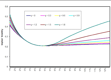
Figure 3.1: F0 = 0.0325, u0 = 0.087, á = 0.47, 9 = 0.7, p = -0.48, T = 15Y

Increasing 'y lifts the wings of the implied volatility smile whereas the smile for strikes close to at-the-money are visibly unaffected. This can in turn be used to give us better control over the CMS prices.

Here is an illustration of how to control CMS prices through the wings. When we increase á, we lift the wings and therefore raise the CMS prices. We can then decrease 'y and therefore lower back the wings and the CMS prices, as we can see it through the following illustration.

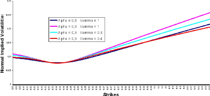
Figure 3.2: F0 = 0.0325, u0 = 0.087, 9 = 0.7, p = -0.48, T = 15Y

In terms of computation time, we have plotted the time it takes to compute an implied volatility in a ZABR('y = 1) and compared it with the time taken by Hagan

CHAPTER. 3. THE ZABR. MODEL

and Labordere approximations.

Figure 3.3: F0 = 0.0325, ó0 = 0.087, á = 0.47, â = 0.7, ñ = -0.48, ã = 1, T = 15Y

It takes 10 times more time for computing implied volatility under the ZABR model, in comparison with Hagan and Labordere approximations. However, this is just the price to pay for gaining control of the wings !

3.3 Fast calibration of the model's parameters

For quick identification of the model parameters, the following second-order Taylor expansion is convenient:

v(K) = v(F) + v^,(F)(K - F) + ¹₂v^,,(F)(K - F)² + O ((K - F)³) v(F) = ó0?(F)

1 v^,(F) =₂ hó₀^-1 ñá + ó0? (F)i

v,,(F) _{6ó0?(F)hó02(7-1)} ((-5 + 2ã)ñ² + 2) + óô (2?(F)?^,,(F) - ?^,(F)²)i

(3.37)

Let's consider a CEV case where we set ?(K) = ù (K-F )â

have:

(F -F )â and ó0 = 1. Then we

v(F) = ù v^,(F) = 21 [~ ñá + Fùâ - F ~~(-5 + 2ã)ñ^2 + 2 á2 + ù^2â(â - 2) ~ v^,,(F) = 1 6ù (F - F)^2 3. EXPANSION FOR. THE ZABR. MODEL

(3.38) 29

CHAPTER 3. THE ZABR MODEL

	\ v(K1), ...,			For a given set of discrete quotes

be used for regressing the triple v(F), v'(F), v"(F). One can in turn solve 3.38 to get parameters estimates for â, ñ, á.

4 Finite difference volatility

Using the implied volatility coming from the short-maturity expansions 3.16, 3.26 and 3.35, directly for pricing using 3.3 will not give arbitrage-free options prices. Our short-maturity expansions suffer from the same problem of potential negative implied densities for low strikes as the original Hagan expansion. The ZABR model contains an enhanced feature that can help us avoid negative density problems. Let's plot the implied probability density function for extreme model parameters and see how it reacts to the changes in ã values.

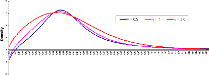
Figure 3.4: F0 = 0.0325, ó0 = 0.087, á = 0.47, â = 0.7, ñ = -0.48, T = 15Y

If we keep increasing ã, the density tends to be more and more positive... Anyway, this way of skipping negative densities doesn't give us enough flexibility in the use of the ZABR model.

In order to definitely avoid this problem, we will instead use the forward volatilities derived in 3.29 and 3.36 as the basis for our pricing.

The forward volatility V(K) can be used to generate option prices as the solution of the Dupire forward PDE (see [5]).

?C(T,K)

?T =

?

?

?

2V(K)2 ?2 ?(T2,K)

C(0, K) = (F - K)⁺

(3.39)

30 4. FINITE DIFFERENCE VOLATILITY

The usual way of solving this numerically is to set up a time discretisation with multiple time steps and then use a finite difference solver. However, to gain speed, we will instead use the single time step implicit finite difference approach introduced in [15]. Here we need to solve the ODE:

C(T, K) - ₂T è(K)2?2C(T, K)

1 ?K2 = (F - K)⁺ (3.40)

4. FINITE DIFFERENCE VOLATILITY 31

CHAPTER 3. THE ZABR MODEL

Z0

It is shown in [15] that this approach generates a set of arbitrage-free call prices for any choice of è. It is also shown that the one-step finite difference price is the Laplace transform of the solution to 3.39. The Laplace transform of the Gaussian distribution is the Laplace distribution:

8 t/T 1 F - Kl T

IF K|

vt

vt

dt = e 2v2 (3.41)

v

v

2v²

which is peaked at K = F. Therefore if we choose è = V, we will also get a peak in the densities.

Instead, we will find an adjustment for the forward volatility function based on our expansion results. As option prices generated by 3.39 and 3.40 should be the

same, we can substitute ?²C(T,K) ?C(T,K)

?K2 = 2 ?T from 3.39 into 3.40 and rearrange to V2

find:

è(K)^2 = V(K)2 C(T, K) - (F - K)^+ T ?C(T,K) ?T V(K)2g(T, F,v) - (Fv) - K)^+ T ?g(T ?T

(3.42)

~ ~

1 - î Ö(-î)

= 2V(K)² , with î= v X

ö(î) T

= V(K)²P(X)²

where the second (approximated) equality involves the approximation of the option prices by our expansion result.

The function P(X)² can conveniently be approximated with a third or fifth order polynomial. Specially:

Ö(X) X

ö(X) a_nuⁿ, u = 1 (3.43) 1 + pX

n

where the constants p, a1, a2, ... can be found in (26.2.16) and (26.2.17) of [20]. The finite difference discretisation of 3.40 is:

~ ~

1- ¹ 2Tè(K)2 ?2 C(T, K) = (F - K)⁺ (3.44)

?K²

This equation can be represented as a tridiagonal matrix equation on the grid K0, K1, ..., K_n, which in turn can be solved for C(T, Ki) in linear CPU time using the tridiag() algorithm in [31].

As an alternative to the finite difference solution 3.44, one could use the exact solution methodology for ODEs of the type 3.40 described in [3]. However, for this methodology to be computationally effective, the forward volatility function è(K) needs to be well approximated by a piecewise linear function with few knot points over the full domain of the solution. This is generally not the case here. We have therefore chosen to base our solution on 3.44.

We can see that the finite difference generated option prices have corresponding implied densities that are positive, that is, arbitrage is precluded. We can also

CHAPTER 3. THE ZABR MODEL

see that using our forward volatility result, V(K), directly in the single time step finite difference solver produces a density that is peaked around at-the-money. This, however, is eliminated when using the adjusted forward volatility è(K).

5 Calibrating the Volatility function

We first consider the case where we have a continuous curve of arbitrage-free option prices. This could for example be produced by Andreasen & Huge interpolation scheme ( [15]) or come from another ZABR model. We can calculate the forward volatility function by the discrete Dupire equation:

è(K)² = ₂C(T, K) - (F - K)+ (3.45)

T ?2C(T,K)

?K²

Using 3.36, we can calibrate the volatility function:

F (Y, óã-1

₀ X) è(K)

?(K) = (3.46)

ó0P(X)

?Y

where X and Y are found from 3.35 as the solution to the ODE system:

ó₀ P (X)

ã-1

?K =

è(K)F (Y, óã-1 0 X)

?X P(X) (3.47)

?K = è(K)

X(K = F) = Y (K = F) = 0

The above ODE system can be solved for all strikes in one sweep. However, typically, we prefer to calibrate directly to the observed discrete quotes. This is done by solving the ODEs in 3.35 and 3.36 and including the one-step finite difference adjustment 3.42:

?Y		óã-2 0
?(K)

?X ?K =

F (Y, óã-1

₀ X)

(3.48)

ó0?(K)

P(X)ó0?(K)

è(K) = F (Y, óã-1

₀ X)

X(K = F) = Y (K = F) = 0

32

5. CALIBRATING THE VOLATILITY FUNCTION

After solving numerically the above system, we can find the option prices using the one-step finite difference algorithm in 3.44. On top of this, we can use a nonlinear solver to calibrate the volatility function ó(K) to observed discrete option quotes. As we get all option prices in one sweep, we can include CMS forwards and option quotes in the calibration without additional computational costs.

CHAPTER 3. THE ZABR MODEL

Even though non-linear iteration is involved, this procedure is very fast. Typically, we can calibrate a non-parametric volatility function with 10 knot points to a given smile in roughly 50 iterations, which takes approximately one millisecond of CPU time.

When it comes to outright pricing speed, the ZABR model is capable of generating 100'000 smiles, each consisting of 256 strikes in approximately seven seconds. It should be stressed that this includes both numerical ODE and finite difference solutions. This is actually faster than direct use of Hagan's SABR expansion, which takes 10 seconds for the same task. The reason for this difference is mainly that one time-step finite difference is faster at producing prices than the Black formula. An alternative to the ZABR model for producing arbitrage-free options prices is the Fourier-based models, found in [2] for example. For a displaced Heston model (see [1]), numerical solution for 100'000 smiles consisting of 256 strikes via the fast Fourier transform with the Black-Scholes formula used as a control variate takes around 18 seconds (see [14]). It should be noted that this type of model is considerably less flexible with respect to fitting discrete quotes and more difficult to implement.

Though we generally use 3.48 in conjunction with a non-linear solver for the calibration, the direct calibration methodology 3.47 is relevant as it admits direct calibration of one ZABR model to another.

The stochastic process _(Xt)t has unit diffusion and thus, in the sense of the short-maturity limit, is normally distributed. So it is natural to use a uniform spacing in X and a non-uniform spacing in K. For this, the ODE system 3.48 can conveniently be transformed to:

?Y			óã-1 0				?K =
F (Y, óã-1 0 X)		?K
ó0?(K)

?X =

(3.49)

F (Y, óã-1

₀ X)

P (X)ó0?(K)

è(K) = F (Y, óã-1

₀ X)

Y (X = 0) = 0, K(X = 0) = F

In our implementation, we solve 3.49 on a uniform X grid to generate and fix a non-uniform strike grid k0, k1, ... , k_n that is used in the numerical solution of 3.48 during calibration and pricing. As a final remark, we note that ODEs in this section typically will be solved at ó0 = 1.