Zabr modelling

Conclusion for the ZABR model

We have used a simple method to derive short-maturity expansion for forward volatilities from stochastic volatility models. The solution is an ODE that can be solved numerically for all strikes in one sweep. Finally, we used a one-step finite difference scheme to generate option prices. That approach is very fast and it generates arbitrage-free option prices. We have added flexibility to the original SABR model to get an exact fit of all quoted option prices and better control of the

5. CALIBRATING THE VOLATILITY FUNCTION 33

34 5. CALIBRATING THE VOLATILITY FUNCTION

CHAPTER 3. THE ZABR MODEL

wings of the smile for improved CMS pricing. Also, we can add CMS prices to the calibration without additional computational costs.

35

Conclusion

This research internship focused on solving two main problems encountered with the SABR model in the financial industry:

· an arbitrage problem observed through the negative density of the underlying,

· a lack of flexibility in wings control

We first developed the Normal SABR model and solved the negative density problem (Chapter 2). We then solved the wings control problem by another model, the ZABR model, which is just an extension of the SABR model where one replaces the (usually) lognormal volatility process by a CEV volatility process, gaining then a control on the smile's wings through the CEV exponent 'y (Chapter 3). We remarked that a direct use of computed implied volatilities for pricing doesn't yield arbitrage-free prices and we finally used a Markovian Projection and found an equivalent local volatility model that is rather used for pricing.

For each solved problem, we gain accuracy but we pay back a computation time, specially for the Normal SABR model. Anyway, the time lost with the ZABR model is worth the wings control and the arbitrage-free prices obtained. The ZABR model is therefore usable in pricing libraries without additional excessive costs.

Beyond the subjects studied in my internship, as suggested through picture 3.2, one can efficiently hedge against model parameters' risk by using the 'y parameter to thwart the movements of the other model parameters. Here, we did it manually but it can be very interesting to look for particular relationships between 'y and (á, 9, p) in terms of a parametric function that will be calibrated while readjusting the level of 'y according to how the other parameters move. We should therefore look for a stability in the smile shape despite the changes in other parameters of the model. This can be done by matching the slope and the convexity of the obtained smiles around the strike. Numerical resolution yields optimization algorithms.

We can therefore look forward to finding closed form formulas in the ZABR model scope. My idea is to rely on the Labordere's heat kernel expansion on a Riemann manifold; and the research continues...

CONCLUSION

36 CONCLUSION

Appendix A

Numerical pricing under Normal

SABR model

1 Density for Normal SABR

We approximate the density of _(Xt)t at zero, that is, EQ^u [ä(Xt)]. As previously explained, the process _(Xt)t satisfies:

_V

dWt = b0 q(Xt)dW u t?ô

= X0 = F0 - K

where q(X) = 1-2ñáX +á²X², á-á/b0, (W_t^u)t is a zero-drift Brownian motion under Qu, and ô is the first time X hits -K.

This is achieved by defining the following process:

Xt

(I(X)) du = 1ln (V(Xt) - ñ + áX\

_t -- 10Vq(u) á 1 - ñ

1 (1 + ñ)²e^2áI + (1 - ñ)²e^2áI + 2(1 - ñ²)) q(X) = g(I) - 4

The process It - I(Xt) admits the following dynamic:

V b2 01{t<ô}dt

1 + á2X2 t - 2ñáXt

1

dIt = b0dWt?ô - 2

áXt - ñá

37

We define the process At = q(Xt)¹/⁴q(X0)¹/⁴ and observe that:

~ ~

2

dlnAt = dlnñt + -¹ + 31 - ñ á2bo1{t<ô}dt

8 8 q(Xt)

dñt 1

=

ñt 2

áXt - ñá

V1 + á²X²_t - 2ñáXt

b0dWt?ô

The martingale _(ñt)t defines a new measure Qñ and we have:

dIt = b0dW ^Qñ

t?ô

APPENDIX A. NUMERICAL PRICING UNDER NORMAL SABR MODEL

where (W ^Qñ

t )t is a Brownian motion under Qñ.

We observe that:

EQu [ä(Xt)] = q(X0)¹/⁴E^Qu [Atä(Xt)] = q(X0)¹/⁴Ë(t)E^Qñ [ä(Xt)]

[exp (-₈ á2b20(t t?ô 11= EQñ ? ô) + ³á²b²₀(1 -82) _o du g(Iu)du)) /It = 0J

Ignoring the stopping time in above expression for Ë(t) and using áb0 = á, we derive:

Ë(t) e- _a á2t × Ö(t, I0

b0

(:á²(1

¹z) = E^Qñ [exp - ñ2) t f(W?)) /W^Qñ = zJ

1 f(W) = 4 ((1 + ñ)²e^-2áW + (1 - ñ)²e^2áX + 2(1 - ñ²))

where (W ^Qñ

t )t is a Qñ-Brownian motion with initial value zero.

Since Ö(t, z) depends exclusively on ñ and á, this function can be pre-calculated or alternatively approximated as follows:

Ö(t, z) = exp [á²(1 - ñ2) (f(0) + f(z) / t] + O(t²)

We define ê(t, z) = -¹₈á² + ₁³₆á²(1 - ñ2) (f(0) + _f(z)) + O(t)

Since E^Qñ [ä(It)] = E^Qñ [ä(Xt)], we finally derive using the reflection principle for Brownian motions:

EQu [ä(Xt)] = q(X0)1/4

b0 v2ðt

I(F0 - K)

B=

2I(Fmin - K) - I(F0 - K)

_v2 , C = _v2

B2 - C2

× ef0 ê(s,b00)ds × [eTht - e bit

38 2. COMPUTATION OF FUNCTIONS Ö AND ê

2 Computation of functions Ö and ê

We propose a simple algorithm to calculate the functions Ö and ê. Let's choose a time grid {Ti : i = 0, ... , N} such that T0 = 0, TN = T and we simplify the computation of Ö(Ti, B) with the following approximation:

IE [exp

3 ^Tz dul l(z) (₈á²(1 - ñ2) Jo ?(Wu)/ I W_T% = zJ

Then, we calculate Øi : î 7? Öi (îvTi) on a set of symmetric Hermite nodes that appear in the Gauss-Hermite integration. One chooses M = 2m for a symmetric set and {îk : k = 1, ..., M} such that:

APPENDIX A. NUMERICAL PRICING UNDER NORMAL SABR MODEL

E [f(î)] = _XM pkf(îk).

k=1

We can calculate Øi by forward induction:

Øi(îk) E [Øi-1(æTi-1) exp (ëÄTi 1 J /æTi = îkJ exp (1ÄTi 1

40(si-1æTi-1)/ \ ~(siîk)
si =pTi ë = ₁₆á²(1 - ñ²), æt =_NAWt.

The conditional expectation can be analytically computed since æTi-1 and æTi are unit normal variables with correlation

ñi =q Ti .

Let's consider the following function:

Fi-1(z) = Øi-1(z) exp ~

ëÄTi 1

?(si-1z)

Then we have:

~ Øi(îk) = E Fi-1(ñiîk + q1 - 401 exp(ëÄTi₍¹₎)

Using the decomposition of Fi-1(z) in its basis cubic spline functions, we can write:

Fi-1(z) = _XM Fi-1(îj)èj(z). j=1

By integrating the above, we can simplify the former equation as follows:

Øi(îk) =

XM j=1

~ tt ëÄT ëÄTi pkj x Øi-1(S9) ^x exp itt + ?(si-1sj) ?(siîk))

ci(z) = A1i (z - îi)³ + B1i (z -îi) - A0i (z - îi+1)³ - B0i (z - îi+1) Lil0 = îi, L0 = -50, Ui6=M = îi+1, UM = 50.

2. COMPUTATION OF FUNCTIONS Ö AND ê 39

~ ~ _q ~~

pkj = pkj(ñi) = E

⁽ⁱ⁾ èj ñiîk + 1 - ñ2 i æ

where p(i)

kj satisfies _{Pj p}(i)

kj = 1 but can be negative.

A crucial observation for time saving is the fact that the pseudo-transition proba-

bilities pkj only depends on the mesh îk and the grid Ti. Consequently, the respective

expectations only need to be computed once.

We can analytically calculate the pseudo-transition probabilities. The function

èj is a cubic spline with value zero at every node except at z = îj where it takes

value 1.

èj(z) = _XM 1{Li<z<Ui}ci(z),

i=1

APPENDIX A. NUMERICAL PRICING UNDER NORMAL SABR MODEL

where A0i, B0i, A1i, B1i are calculated using the standard cubic spline algorithm. We finally compute the pseudo-transition probabilities:

pkj(ñ) = _XM ñ³? _[A1iI3(li, ui, vi) - A0iI3(li, ^ui, vi+1)] + ñ? _[B1iI1(li, ui, vi) - B0iI1(li, ^ui, _vi+1)] , i=0

Li - ñîk li = (1 - ñ2)1/2, ui =

Ui - ñîk (1 - ñ2)1/2, vi =

ñîk - îi p (1 - ñ2)1/2, ñ? = 1 - ñ2

Where I_n(a, b, c) = E [1{a<î<b}(î + c)ⁿ]. By integration, we obtain:

I1(a, b, c) = c [N (b) - N(a)] + f_z(a) - f_z(b)

I3(a, b, c) = (c² + 3c)[N(b) - N(a)] + [3c(c + a) + a² + 2] f_z(a) - [3c(c + b) + b² + 2] f_z(b)

where fZ(.) is the Gaussian density.

40 2. COMPUTATION OF FUNCTIONS Ö AND ê

41

Appendix B

Equivalence between Normal and

Log-normal Implied Volatility

Asymptotics of implied volatility are important for different reasons. On the one hand, they give information on the behaviour of the underlying through the moment formula [29] or the tail-wing formula [30]. On the other hand, they allow a full correspondence between vanilla prices and implied volatilities. With such a correspondence, asymptotics in call prices can be easily transformed into asymptotics in implied volatilities. When applied to a specific model, asymptotics are widely used as smile generators [26]. In practice, other models are then used for pricing options using tools like Monte-Carlo simulations.

So far, all the asymptotics studied by authors concern asymptotics for implied lognormal volatility. In this chapter, we consider implied normal volatility which refers to the Bachelier model. Why is it interesting to consider normal implied volatility? One the one hand, for short maturities, the Bachelier process makes more sense than the Black-Scholes model. Indeed, the behaviour of the underlying from one day to another is generally well approximated by a Gaussian random variable [32]. That's the reason why the Bachelier model is very popular in high frequency trading [21]. On the second hand, the "breakeven move" of a delta-hedged option is easily interpreted as normal volatility. Generally, the P&L of a book of delta-hedged option is positive if the (historical) volatility of the underlying is greater than a breakeven volatility which has to be expressed in normal volatility. Moreover, it makes more sense to compare implied normal volatilities with historical moves of the underlying as can be done by a market risk department. Likewise, some markets such as fixed-income markets with products like spread-options are quoted in terms of implied normal volatility [16]. Finally, the skewness of swaption prices is much reduced if priced in terms of normal volatility instead of lognormal volatility. Therefore, it is important to have a robust and quick way to compute implied normal volatilities from market prices and also to be able to switch between lognormal volatilities and normal volatilities.

What kind of asymptotics should we consider? Most of the approximations in option pricing theory are made under the assumption that the maturity is either small (see the Hagan et al. formula [26]) or large [17]; it is actually assumed that

42 1. ANOTHER PRICING FORMULA FOR CALL OPTIONS IN THE BACHELIER MODEL

APPENDIX B. EQUIVALENCE BETWEEN NORMAL AND LOG-NORMAL IMPLIED VOLATILITY

a certain time-variance U²T is either small or large. A possible way to derive such approximations is to replace the factor of volatility U by EU and then set E = 1. This can be done at the partial differential equation level (see all the techniques coming from physics [26]) as well as directly at the stochastic differential equation level with the help of the Wiener chaos theory for instance [33]. Other types of asymptotics are obtained by considering large strikes. In our approach, we unify all those types of asymptotics (see [18] and [9] for the lognormal case). Indeed, we obtain an approximation of the implied normal volatility as an asymptotic expansion in a parameter À for À « 1 and it turns out that À -+ 0 when T -+ 0 or K -+ +00.

This study is organized as follows. We first give another expression for the pricing of a European call option which involves an incomplete Gamma function (Proposition 1.1). Then, we inverse this function asymptotically and obtain an expansion of normal implied volatility. This is particularly important if we want to quickly obtain the implied normal volatilities from call prices as is the case in high frequency trading [21]. The formula is also potentially useful theoretically if, given an approximation for the price of a European call option or a spread option (for instance in the framework of the Heston or the SABR model), we want to obtain an approximation of the normal implied volatility. Finally, we restrict our formula to the order 0 and we compare it to a similar formula for the lognormal case. Then, we obtain an equivalence between normal volatility and lognormal volatility. We use it also to compare the Black-Scholes greeks to the Bachelier greeks. Finally, we consider a delta-hedged portfolio and we compute the breakeven move in the normal case as well as in the lognormal case.

1 Another pricing formula for call options in the Bachelier model

In the Bachelier model, the dynamic of a stock _(St)t?R+ is given by:

( dSt = UNdWt,

(B.1) S0 = S

The so-called normal volatility UN is related to the price of a call C(T, K) struck at K with maturity T by the following formula:

(S - K ) (S - K )

\/

C(T, K) = (S - K) \/ + UN T f_z \/ ,

UN T UN T

(B.2)

( ) Z x

1 _-x²

with f_z(x) = _\/2ð exp and (x) = fZ(u)du.

2 -8

Following Ropper-Rutkowski [23], we can isolate the volatility UN in the pricing formula.

APPENDIX B. EQUIVALENCE BETWEEN NORMAL AND LOG-NORMAL IMPLIED VOLATILITY

Definition 1.1. Let us denote by TV (K,T) (or simply TV ) the time-value of a European call option struck at strike K with maturity T. Then TV (T, K) := C(T, K) - (S - K)+ .

Proposition 1.1. In the Bachelier model, we

TV (T, K) =

{

1 (S-K)^2 if K =6S, 4vð 2^, 2ó^2NT v óN v2ð otherwise T

(B.3)

where (a, z) is the incomplete Gamma function:

(a, z) =

+8

ua-1 exp(-u)du

_f

v

Proof. We have C(T,K)

S = f(î, è) with î := K S and è := óN S and

T

f(î,u) := (1 - î)N \1 - î /u + ufz \1 u
By differentiation, we have:

?u(î,u)=-(1u2î)2fz \1u/+- _îfzu- î_u 1 --

2

_u2¹

/ \ u/fz\1u/

fz

\1 -î/

u

where we have used fz(î) = -îf_z(î). Since f(î, 0) = C(0,K)

S = (1 -î)+ , we

deduce that:

f(î,è) = (1 -î)+ + _fB /1 u

fz ( I du

o \ If we set

F(î, è) :=f^B fz ( \1 u du

o

then we have:

C(T, K) S

Kv ! = (1 - î)+ + F S , ó T S

Let's assume that both è =6 0 and î =6 1. With the change of variable v := 1-î

_u ,

we get:

+8 F(î,è) = |1 -î| f1 î| è

fz(v) dv v2

So, with a new change of variable u := ¹₂v², we have:

1. ANOTHER PRICING FORMULA FOR CALL OPTIONS IN THE BACHELIER MODEL 43

APPENDIX B. EQUIVALENCE BETWEEN NORMAL AND LOG-NORMAL IMPLIED VOLATILITY

Z +8 1 F(î, è) = 4vð |1 - î| ~2 2è

u-

3 2 exp(-u)du

4vð1 |1 - î|(-¹₂,|¹_2è2|²₎

v2ð

where (a, z) is the incomplete Gamma function. At the money, we simply have C(T, K) = óNvT

It's clear from Proposition 1.1 that the real-valued function T 7? C(T, K) is non-decreasing, positive, C(0, K) = (S - K)+ and _limT?+8 C(T, K) = +8. So, given the price of a European call option C, there is a unique real number óN(T, K) such that C(T, K) = C with a normal volatility óN = óN(T, K). We say that óN(T, K) is the normal implied volatility

Remark 1.1. We can easily see that _|Ks| depends only on ^arKT (only one variable).

One of the interests of Proposition 1.1 is that there are efficient algorithms to compute the inverse of the incomplete Gamma function. In particular, it is implemented in Matlab. Therefore, it is always easy to get the implied normal volatility from call prices [22]. Such a task is not always easy in the lognormal case [28], especially when we are far from the money.

Corollary 1.1. Let p be an integer. Then,

(ó

TV T K) = NT) 2 ex _(S - K)2 p-1 1 k (2k + 1)! óNT ^k + R

TV( v2ð(S - K)2 p ( _2ó2NT ) ( ) k! ((S - K)2) p

k=0

with |R_p| = (2p + 1)! 011¹011^1P

p! ( (S - K)2 )

(B.4)

The above equation comes naturally from a well known asymptotic expansion of (a, z) for large z (see Formula 6.5.32 in [20]).

Remark 1.2. From either pricing formula B.2 or B.3, we can notice that we can use the same trick to price large strike and short maturity European options (as expansions in both cases are similar)... This comes from the fact that:

C(ë²T, ëS + (1 - ë)K) = ëC(T, K) for any non-negative real ë. This is particular to the Bachelier model.

For a comparison with the lognormal case, it can be advantageous to introduce the following notations.

44 1. ANOTHER PRICING FORMULA FOR CALL OPTIONS IN THE BACHELIER MODEL

APPENDIX B. EQUIVALENCE BETWEEN NORMAL AND LOG-NORMAL IMPLIED VOLATILITY

Definition 1.2. For K 6=, we set èN := óN s T xN := -1, ãN := log (4vð),

uN :=

|xN |

2è2 - 1

log(TV (T,K)

N

_S ).

x

Then by Corollary 1.1, for K =6 S and p ? N^*,

4vð		TV (T, K)	= u	3/2 e N	1 uLN	X p-1 k=0	(1)^kk k 2k aLNuLN + RpLN
|xN|		S

(B.5)

(B.6)

~

2 /

with uLN := ~LN, èLN := óLNV ^T, xLN := log C S , R^p_LN ? Ù (èx) , xLN

1 x2 i

^LN and(2k + 1)!! := 11(2j + 1).

j!(2j + 1)!! 8

aLkN := (2k + 1)!! _Xn

k=0

j=0

Here, óLN denotes the lognormal implied volatility.

2 Asymptotics of the implied normal volatility 2.1 First and Second order expansion

-

3/2

1 u_N

u

X p-1 k=0

N e

Let us assume that K =6 S. Using B.5, we get:

ukuN + O (u_N))

= eãNe-1/ë

with uk :=

(-1)^k 2k ak

Therefore, by Lemma 1 of [9], we get the following proposition.

Proposition 2.1. Let us denote by TV the time-value of a European call option, óN its implied normal volatility and T the maturity of the option. Set ë := - 1

log(T SV ),

ãN := log

(4_|x,z)

and xN = KS - 1. Let's assume that K =6S. Then, in the case when T ? 0, we have the following expansion for the time-variance of the call option: ó²_NT = (S-K)2

₂ uN with

³_²_²⁹_³_²/⁹ _ \ 3 log(A)

+ (ã²_N -³₂ãN + 2) A3 + o(ë³) (B.7)

In the lognormal case [9], for short expiries, the asymptotic expansion of ó2LNT is

2. ASYMPTOTICS OF THE IMPLIED NORMAL VOLATILITY 45

APPENDIX B. EQUIVALENCE BETWEEN NORMAL AND LOG-NORMAL IMPLIED VOLATILITY

given by ó2LNT = log2(K/S)

2 uLN with

99

uLN =ë - ₂ë²log(ë) +ãLNë² + ₄ë³log²(ë) + 14 - 3ãLN I ë3log(ë)

(N - ë3 + o(ë³)

+ ₂ãLN - u₁ (B.8)

LN := log

XLN 2

-

ã

4vðex ² and ui:= - LN| 16 2

First, we note that ë = uLN + o(uLN). Then comparing the two results B.7 and B.8 for K =6 S, we obtain:

uN = uLN + (ãN - ãLN)u²LN + O (u3LN log(uLN))

So,

~SxN 2

_ó2 LNT + O ~T² log(T)~ (B.9)

N = ó²_LN + 2(ãN - ãLN)S2x2 Nó4

xLN x4 _LN

Since ^xN xLN

S-K = log(S)-log(K) > 0, we deduce that

~ 1/2

SxN

óN =

xLN

SxN

=

xLN

1 + 2(ãN - ãLN)ó2 ^LN + O ~T² log(T)~

óLN T

x2 _LN (B.10)

2 1/2

ó

ã

-ã

^ó

x

LN (1 + (

N

LN)

2NT) + O (T2 log(T))

LN

46 2. ASYMPTOTICS OF THE IMPLIED NORMAL VOLATILITY

Moreover, we have:

Hence, we get: K

ãN - ãLN =

~xLN ~ xLN 2 + log xN

S

? ~S-K ~ ?

-

log ,/KS(log S-log K) ?+ O ~T 2 log(T)~

óN = log(S) - log(K)óLN _?1 - (log S - log K)2 ó2 LNT

Note also that at the money, the situation is quite easy. On the one hand, we have (cf. Proposition 1.1)

_r

2ð

óN = T C

On the other hand, we have ( [9], Proposition 2.1):

v !

óLN T

C = erf 2v2

Therefore, we state the following result.

APPENDIX B. EQUIVALENCE BETWEEN NORMAL AND LOG-NORMAL IMPLIED VOLATILITY

Corollary 2.1.
· if K =6 S, we have:

UN =	2 S-K S - ^KULN 1 - log KS(log S-log K) U2 T + O (T^2 log(T) log S - log K (log S - log K)2 LN

(B.11)

In particular, UN ~

S-K

log S-log KULN when T ? 0.

· At the money, we have UN = /2ðerf óLNT and UN

SULN 1 aLNT

2v2=- +

24

o(T).

In particular, UN ~ SULN when T ? 0.

Remark 2.1. When K ? S, we can check that In other terms, for K =6 S,

S-K log vKS(log S-log K) 1 (log S-log K)^2 24

ULN =

S(m m1) UN, where m = S = xN + 1 is the Moneyness. (B.12) This formula was known (even if it was not stated explicitly) in the SABR model (see Hagan et al. formula [26] ). By differentiatinf Formula B.12 with respect to m, it turns out that the Black-Scholes skew ?óLN

?m at the money (m = 1) generated by

the Bachelier model is ?óLN

?m = _-1 óN S (ULN is by definition the implied lognormal 2

volatility). Therefore, the Bachelier model is highly skewed ATM (a slope of -50%× óNS ). Another way to explain this feature is that given call prices, when we use the BS model, the function ULN is a decreasing and convex function of m, i.e., it generates a skew, while the function UN is a rather flat function of m. Thus, normal volatility is most suited for products such as swaptions for instance.

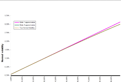
2.2 Accuracy of asymptotic expansions

Here we address the question of the accuracy of our expansions. Therefore, we proceed by backward induction of the lognormal implied volatility as described bellow:

· Let's choose several random lognormal implied volatility and compute a Call price through Black & Scholes formula without interest rate

· From each Call price, we calibrate the volatility parameter from a Bachelier model by numerical inversion of the pricing formula. We therefore obtain the likely "true" normal implied volatilities equivalent to our initial lognormal volatilities

· For comparison, we respectively apply the first and second order approximations with our initial lognormal implied volatilities and we obtain other normal volatilities that we can compare with the former ones

Applying the above process leads to the following curve where we have plotted comparison curves for different maturities.

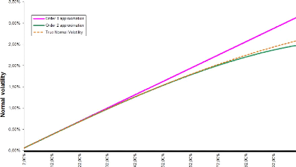
The first order approximation supposes an affine relationship between normal and lognormal implied volatilities whereas the second order supposes a parabolic one. We can observe that the raise of the maturity deteriorates our asymptotic expansions. The more we increase the option's expiry, the more our approximation is credible.

2. ASYMPTOTICS OF THE IMPLIED NORMAL VOLATILITY 47

48 2. ASYMPTOTICS OF THE IMPLIED NORMAL VOLATILITY

APPENDIX B. EQUIVALENCE BETWEEN NORMAL AND LOG-NORMAL IMPLIED VOLATILITY

- Order 1 approximation

- Order 2 approximation --- True Normal Volatility

2,50% -

2,90% -

ô ô

V

3,50% -

3,00% -

Lognormal volatility

Figure B.1: T = 1, F₀ = 0.0325, K = 0.03

- Order 1 approximation

- Order 2 approximation --- True Normal Volatility

3,09%

3,50%

2,50%

2,99%

0,59%

0,0C%

V V V

ô ô ô ô ô

N N N N

V

Lognormal volatility

Figure B.2: T = 1, F₀ = 0.0325, K = 0.03

APPENDIX B. EQUIVALENCE BETWEEN NORMAL AND LOG-NORMAL IMPLIED VOLATILITY

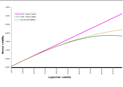
Figure B.3: T = 1, F0 = 0.0325, K = 0.03

3 Comparing greeks and delta-hedged portfolios

Let's denote by ON, FN, íN, ÈN (resp. OLN, FLN, íLN, ÈLN), the delta, gamma,

vega and theta in the Bachelier (resp. Black-Scholes) model. For instance, íN = ?C

?óN .

By differentiating B.2, we get:

CS - K)

ON = N (B.13)

óN vT

On the other hand, it is known that:

OLN = _NClnS - lnK 1 1

+ (B.14)

óLNv T 2ULN T)

So, by Corollary 2.1, we get: OLN ~ ON for a maturity T « 1. By differentiating B.13, we obtain:

ü fz CS ) (B.15)
FN =

óN T óN T

In the Black-Scholes model, we have:

= 1 ClnS - lnK 1 )

FLN SóLNvT fz óLNvT + ₂óLNvT (B.16)

Hence, with the help of Corollary 2.1,

lnS - lnK

FN ~ S - K FLN (B.17)

Now we consider the Vega. It is shown above that:

3. COMPARING GREEKS AND DELTA-HEDGED PORTFOLIOS 49

APPENDIX B. EQUIVALENCE BETWEEN NORMAL AND LOG-NORMAL IMPLIED VOLATILITY

C(T, K) = (S - K)+ + S 0

v óN T S

f(1 - K/S ) ^zu du

So, differentiating w.r.t. óN, we get:

/ (S - K)²

íN T = S 2ð 2T 2~² T ) (B.18)

N

In contrast, the vega in the Black-Scholes model id

/T ((lnS - lnK +₂óTNT)²)

íLN = S _2ð exp (B.19)

2ó2 LNT

Likewise, we can compare the two thetas. We then have the following proposition

Proposition 3.1. When T ? 0, and under the hypothesis of bounded volatilities, we have:

ÄN ~ ÄLN íN ~ íLN N S lnS - lnK LN ~ S - K S - K ÈN ~ ÈLN S(lnS - lnK)^ÈLN

(B.20)

The first equivalence ÄN ~ ÄLN shows that hedging in the Bachelier framework is more or less like hedging in a Black-Scholes framework. However, the "breakeven move" of a delta-hedged portfolio is not the same. By definition, the "breakeven move" of a delta-hedged portfolio is the number u such that over a short horizon ät, P&L > 0 if the change in S is > u. In general, we have:

(ÄS)²

1

=

2

1

P &L = -Èät + 2

[(ÄS)² - u²]

(B.21)

So, with ät = 1,

m - ₁uN (B.23)

lnm

uLN =

with m = K/S. So, at the money, uLN ~ uN. However, if K < S (resp. K > S)

then uLN < uN (rep. uN > uLN.

50

3. COMPARING GREEKS AND DELTA-HEDGED PORTFOLIOS

_r

2È

u = .(B.22)

Using Proposition 3.1, we find that the "breakeven move" uLN in the Black-Scholes model is related with the "breakeven move" uN in the Bachelier model by:

3. COMPARING GREEKS AND DELTA-HEDGED PORTFOLIOS 51

APPENDIX B. EQUIVALENCE BETWEEN NORMAL AND LOG-NORMAL IMPLIED VOLATILITY

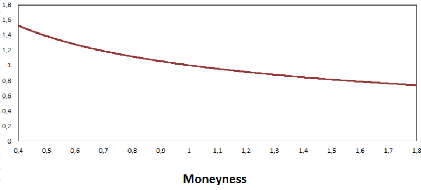
Figure B.4: The volatility smile of the Bachelier model (normalized by the factor óN S where óN denotes the normal volatility

and the ratio of "breakeven moves" uLN/uN.

The following graph represents the function in 7? ln(m)

m-1 which gives the smile

of the Bachelier model (cf Corollary 2.1) as well as the ratio of "breakeven moves" uLN .

uN

So, depending on the view of the trader on the short term dynamic of the underlying (normal or lognormal diffusion), he will adjust or not the "breakeven move"

of his delta-hedged portfolio by the factor lnm

m-1.

APPENDIX B. EQUIVALENCE BETWEEN NORMAL AND LOG-NORMAL IMPLIED VOLATILITY

52 3. COMPARING GREEKS AND DELTA-HEDGED PORTFOLIOS

53

Bibliography

[1] Lipton A. A closed-form solution for options with stochastic volatility with applications to bond and currency options. Review of Financial Studies, 6, 1993.

[2] Lipton A. The vol smile problem. Risk February, 2002.

[3] Lipton A. and A. Sepp. The vol smile problem. Risk February, 2011.

[4] Jesper Andreasen and Brian Huge. Expanded forward volatility. Risk Magazine, 2013.

[5] Dupire B. Pricing with a smile. Risk January, 1994.

[6] Dupire B. A unified theory of volatility. Working paper, BNP Paribas, 1996.

[7] Philippe Balland and Quan Tran. Sabr goes normal. Risk Magazine, 2013.

[8] Eric Benhamou and Olivier Croissant. Local time for the sabr model: Connection with complex black scholes and application to cms and spread options. Working Paper, 2007.

[9] Grunspan C. Asymptotic expansions of the lognormal implied volatility: A model free approach. Preprint, 2011.

[10] E. Derman and I. Kani. Stochastic implied trees: Arbitrage pricing with stochastic term and strike structure of volatility. Int J. Theoritical and Applied Finance, 1998.

[11] B. Dupire, M.A. H. Dempster, and S. R. Pliska. Pricing and hedging with smiles, in mathematics of derivative securities. Cambridge University Press, 1997.

[12] Robert Goldstein and William Keirstead. On the term structure of interest rates in the presence of reflecting and absorbing boundaries. Working Paper, 1997.

[13] Gyongy I. Mimicking the one-dimensional marginal distributions of processes having an itô differential. Probability Theory and Related Fields, 71, 1986.

[14] Andreasen J. and L. Andersen. Volatile volatilities. Risk December, 2002.

[15] Andreasen J. and B. Huge. Volatility interpolation. Risk March, 2011.

54 BIBLIOGRAPHY

BIBLIOGRAPHY

[16] Kienitz J. and Wittke M. Option valuation in multivariate sabr models - with an application to the cms spread. Preprint, 2010.

[17] Fouque JP., Papanicolaou G., Sircar R., and Solma K. Singular perturbations in option pricing. SIAM Journal on Applied Mathematics, 63(5), 2003.

[18] Gao K. and Lee R. Asymptotics of implied volatility to arbitrary order. Preprint, 2011.

[19] Andersen L. and R. Ratcliffe. Extended libor market models with stochastic volatility. Working paper, General Re Financial Products, 2002.

[20] Abramowitz M. and Stegun IA. Handbook of mathematical functions. Dover, 1966.

[21] Avellaneda M. and Stoikov S. High-frequency trading in a limiot order book. Quantitative Finance, 8(3), 2008.

[22] Li M. and Lee K. An adaptative successive over-relaxation method for computing the black-scholes implied volatility. Quantitative Finance, 2009.

[23] Roper M. and Rutkowski M. A note on the behaviour of the black-scholes implied volatility close to expiry. International Journal of Theoretical and Applied Finance, 12(4), 2009.

[24] Balland P. Forward smile. Presentation, ICBI Global Derivatives, 2006.

[25] Doust P. No arbitrage sabr. Working paper, Royal Bank of Scotland, 2010.

[26] Hagan P., Kumar D., Lesniewski A., and Woodward D. Managing smile risk. Wilmott Journal, pages 84 108, Jul 2002.

[27] Henry-Labordere P. Analysis, geometry and modeling in finance. Chapman and Hall, 2008.

[28] Jaeckel P. By implication. Wilmott Journal, nov 2006.

[29] Lee R. The moment formula for implied volatility at extreme strikes. Mathematical Finance, 14(3), Jun 2004.

[30] Benaim S. and Friz P. Smile asymptotics ii: models with known moment generating functions. Journal of Applied Probability, 45(1):16 32, 2008.

[31] Press W., B. Flannery, S. Teukolsky, and W. Vetterling. Numerical recipes in c. Cambridge University Press, 1992.

[32] Schachermayer W. and Teichmann J. How close are the option pricing formulas of bachelier and black-merton-scholes? Mathematical Finance, 18(1):155 170, 2008.

[33] Osajima Y. General asymptotics of wiener functionals and application to mathematical finance. Preprint, 2007.

BIBLIOGRAPHY 55

BIBLIOGRAPHY

[34] Osajima Yasufumi. The asymptotic expansion formula of implied volatility for dynamic sabr model and fx hybrid model. Mitshubishi UFJ Securities Co., 2007.

[35] Osajima Yasufumi. General short-rate analytics. Risk Magazine, 2011.